Advanced Mathematics and Mechanics Applications Using MATLAB phần 1 pptx

CHAPMAN & HALL/CRC
A CRC Press Company
Boca Raton London New York Washington, D.C.
Third Edition
Advanced
Mathematics
and Mechanics
Applications Using
Howard B. Wilson
University of Alabama
Louis H. Turcotte
Rose-Hulman Institute of Technology
David Halpern
University of Alabama
MATLAB
®
© 2003 by Chapman & Hall/CRC

This book contains information obtained from authentic and highly regarded sources. Reprinted material
is quoted with permission, and sources are indicated. A wide variety of references are listed. Reasonable
efforts have been made to publish reliable data and information, but the author and the publisher cannot
assume responsibility for the validity of all materials or for the consequences of their use.
Neither this book nor any part may be reproduced or transmitted in any form or by any means, electronic
or mechanical, including photocopying, microfilming, and recording, or by any information storage or
retrieval system, without prior permission in writing from the publisher.
The consent of CRC Press LLC does not extend to copying for general distribution, for promotion, for
creating new works, or for resale. Specific permission must be obtained in writing from CRC Press LLC
for such copying.
Direct all inquiries to CRC Press LLC, 2000 N.W. Corporate Blvd., Boca Raton, Florida 33431.

Trademark Notice:

Product or corporate names may be trademarks or registered trademarks, and are
used only for identification and explanation, without intent to infringe.

Visit the CRC Press Web site at www.crcpress.com

© 2003 by Chapman & Hall/CRC
No claim to original U.S. Government works
International Standard Book Number 1-58488-262-X
Library of Congress Card Number 2002071267
Printed in the United States of America 1 2 3 4 5 6 7 8 9 0
Printed on acid-free paper

Library of Congress Cataloging-in-Publication Data

Wilson, H.B.
Advanced mathematics and mechanics applications using MATLAB / Howard B.
Wilson, Louis H. Turcotte, David Halpern.—3rd ed.
p. cm.
ISBN 1-58488-262-X
1. MATLAB. 2. Engineering mathematics—Data processing. 3. Mechanics,
Applied—Data processing. I. Turcotte, Louis H. II. Halpern, David. III. Title.
TA345 . W55 2002
620

′

.00151—dc21 2002071267

C262X disclaimer Page 1 Friday, August 2, 2002 11:45 AM
© 2003 by Chapman & Hall/CRC
For my dear wife, Emma.
Howard B. Wilson
For my loving wife, Evelyn, our departed cat, Patches, and my parents.
Louis H. Turcotte
© 2003 by Chapman & Hall/CRC
Preface
This book uses MATLAB
R

to analyze various applications in mathematics and me-
chanics. The authors hope to encourage engineers and scientists to consider this
modern programming environment as an excellent alternative to languages such as
FORTRAN or C++. MATLAB
1
embodies an interactive environment with a high
level programming language supporting both numerical and graphical commands for
two- and three-dimensional data analysis and presentation. The wealth of intrinsic
mathematical commands to handle matrix algebra, Fourier series, differential equa-
tions, and complex-valued functions makes simple calculator operations of many
tasks previously requiring subroutine libraries with cumbersome argument lists.
We analyze problems, drawn from our teaching and research interests, empha-
sizing linear and nonlinear differential equation methods. Linear partial differential
equations and linear matrix differential equations are analyzed using eigenfunctions
and series solutions. Several types of physical problems are considered. Among
these are heat conduction, harmonic response of strings, membranes, beams, and
trusses, geometrical properties of areas and volumes, ßexure and buckling of inde-
terminate beams, elastostatic stress analysis, and multi-dimensional optimization.
Numerical integration of matrix differential equations is used in several examples

illustrating the utility of such methods as well as essential aspects of numerical ap-
proximation. Attention is restricted to the Runge-Kutta method which is adequate to
handle most situations. Space limitation led us to omit some interesting MATLAB
features concerning predictor-corrector methods, stiff systems, and event locations.
This book is not an introductory numerical analysis text. It is most useful as a ref-
erence or a supplementary text in computationally oriented courses emphasizing ap-
plications. The authors have previously solved many of the examples in FORTRAN.
Our MATLAB solutions consume over three hundred pages (over twelve thousand
lines). Although few books published recently present this much code, comparable
FORTRAN versions would probably be signifcantly longer. In fact, the conciseness
of MATLAB was a primary motivation for writing the book.
The programs contain many comments and are intended for study as separate en-
tities without an additional reference. Consequently, some deliberate redundancy
1
MATLAB is a registered trademark of The MathWorks, Inc. For additional information contact:
The MathWorks, Inc.
3 Apple Hill Drive
Natick, MA 01760-1500
(508) 647-7000, Fax: (508) 647-7001
Email:
© 2003 by Chapman & Hall/CRC
exists between program comments and text discussions. We also list programs in a
style we feel will be helpful to most readers. The source listings show line numbers
adjacent to the MATLAB code. MATLAB code does not use line numbers or permit
goto
statements. We have numbered the lines to aid discussions of particular pro-
gram segments. To conserve space, we often place multiple MATLAB statements on
the same line when this does not interrupt the logical ßow .
All of the programs presented are designed to operate under the 6.x version of
MATLAB and Microsoft Windows. Both the text and graphics windows should be

simultaneously visible. A windowed environment is essential for using capabilities
like animation and interactive manipulation of three dimensional Þgures. The source
code for all of the programs in the book is available from the CRC Press website at
. The program collection is organized using an
independent subdirectory for each of the thirteen chapters.
This third edition incorporates much new material on time dependent solutions of
linear partial differential equations. Animation is used whenever seeing the solution
evolve in time is helpful. Animation illustrates quite well phenomena like wave
propagation in strings and membranes. The interactive zoom and rotation features in
MATLAB are also valuable tools for interpreting graphical output.
Most programs in the book are academic examples, but some problem solutions
are useful as stand-alone analysis tools. Examples include geometrical property cal-
culation, differentiation or integration of splines, Gauss integration of arbitrary order,
and frequency analysis of trusses and membranes.
A chapter on eigenvalue problems presents applications in stress analysis, elastic
stability, and linear system dynamics. A chapter on analytic functions shows the
efÞciency of MATLAB for applying complex valued functions and the Fast Fourier
Transform (FFT) to harmonic and biharmonic functions. Finally, the book concludes
with a chapter applying multidimensional search to several nonlinear programming
problems.
We emphasize that this book is primarily for those concerned with physical appli-
cations. A thorough grasp of Euclidean geometry, Newtonian mechanics, and some
mathematics beyond calculus is essential to understand most of the topics. Finally,
the authors enjoy interacting with students, teachers, and researchers applying ad-
vanced mathematics to real world problems.The availability of economical computer
hardware and the friendly software interface in MATLAB makes computing increas-
ingly attractive to the entire technical community. If we manage to cultivate interest
in MATLAB among engineers who only spend part of their time using computers,
our primary goal will have been achieved.
Howard B. Wilson

Louis H. Turcotte
David Halpern
© 2003 by Chapman & Hall/CRC
Contents
1Introduction
1.1MATLAB:AToolforEngineeringAnalysis
1.2MATLABCommandsandRelatedReferenceMaterials
1.3ExampleProblemonFinancialAnalysis
1.4ComputerCodeandResults
1.4.1ComputerOutput
1.4.2DiscussionoftheMATLABCode
1.4.3CodeforFinancialProblem
2ElementaryAspectsofMATLABGraphics
2.1Introduction
2.2OverviewofGraphics
2.3ExampleComparingPolynomialandSplineInterpolation
2.4ConformalMappingExample
2.5NonlinearMotionofaDampedPendulum
2.6ALinearVibrationModel
2.7ExampleofWavesinanElasticString
2.8PropertiesofCurvesandSurfaces
2.8.1CurveProperties
2.8.2SurfaceProperties
2.8.3ProgramOutputandCode
3SummaryofConceptsfromLinearAlgebra
3.1Introduction
3.2Vectors,Norms,LinearIndependence,andRank
3.3 Systems of Linear Equations, Consistency, and Least Squares Ap-
proximation
3.4ApplicationsofLeastSquaresApproximation

3.4.1AMembraneDeßectionProblem
3.4.2 Mixed Boundary Value Problem for a Function Harmonic
InsideaCircularDisk
3.4.3 Using Rational Functions to Conformally Map a Circular
DiskontoaSquare
3.5EigenvalueProblems
3.5.1StatementoftheProblem
3.5.2ApplicationtoSolutionofMatrixDifferentialEquations
© 2003 by Chapman & Hall/CRC
3.5.3TheStructuralDynamicsEquation
3.6ComputingNaturalFrequenciesforaRectangularMembrane
3.7ColumnSpace,NullSpace,OrthonormalBases,andSVD
3.8ComputationTimetoRunaMATLABProgram
4MethodsforInterpolationandNumericalDifferentiation
4.1ConceptsofInterpolation
4.2Interpolation,Differentiation,andIntegrationbyCubicSplines
4.2.1ComputingtheLengthandAreaBoundedbyaCurve
4.2.2Example:LengthandEnclosedAreaforaSplineCurve
4.2.3GeneralizingtheIntrinsicSplineFunctioninMATLAB
4.2.4Example:ASplineCurvewithSeveralPartsandCorners
4.3NumericalDifferentiationUsingFiniteDifferences
4.3.1Example:ProgramtoDeriveDifferenceFormulas
5GaussIntegrationwithGeometricPropertyApplications
5.1FundamentalConceptsandIntrinsicIntegrationToolsinMATLAB
5.2ConceptsofGaussIntegration
5.3ComparingResultsfromGaussIntegrationandFunctionQUADL
5.4GeometricalPropertiesofAreasandVolumes
5.4.1AreaPropertyProgram
5.4.2ProgramAnalyzingVolumesofRevolution
5.5 Computing Solid Properties Using Triangular Surface Elements and

UsingSymbolicMath
5.6NumericalandSymbolicResultsfortheExample
5.7GeometricalPropertiesofaPolyhedron
5.8EvaluatingIntegralsHavingSquareRootTypeSingularities
5.8.1ProgramListing
5.9GaussIntegrationofaMultipleIntegral
5.9.1Example:EvaluatingaMultipleIntegral
6FourierSeriesandtheFastFourierTransform
6.1DeÞnitionsandComputationofFourierCoefÞcients
6.1.1TrigonometricInterpolationandtheFastFourierTransform
6.2SomeApplications
6.2.1UsingtheFFTtoComputeIntegerOrderBesselFunctions
6.2.2DynamicResponseofaMassonanOscillatingFoundation
6.2.3GeneralProgramtoPlotFourierExpansions
7DynamicResponseofLinearSecondOrderSystems
7.1SolvingtheStructuralDynamicsEquationsforPeriodicForces
7.1.1ApplicationtoOscillationsofaVerticallySuspendedCable
7.2DirectIntegrationMethods
7.2.1ExampleonCableResponsebyDirectIntegration
© 2003 by Chapman & Hall/CRC
8IntegrationofNonlinearInitialValueProblems
8.1 General Concepts on Numerical Integration of Nonlinear Matrix Dif-
ferentialEquations
8.2 Runge-Kutta Methods and the ODE45 Integrator Provided in MAT-
LAB
8.3Step-sizeLimitsNecessarytoMaintainNumericalStability
8.4 Discussion of Procedures to Maintain Accuracy by Varying Integra-
tionStep-size
8.5ExampleonForcedOscillationsofanInvertedPendulum
8.6DynamicsofaSpinningTop

8.7MotionofaProjectile
8.8ExampleonDynamicsofaChainwithSpeciÞedEndMotion
8.9DynamicsofanElasticChain
9BoundaryValueProblemsforPartialDifferentialEquations
9.1SeveralImportantPartialDifferentialEquations
9.2SolvingtheLaplaceEquationinsideaRectangularRegion
9.3TheVibratingString
9.4ForceMovingonanElasticString
9.4.1ComputerAnalysis
9.5WavesinRectangularorCircularMembranes
9.5.1ComputerFormulation
9.5.2InputDataforProgrammembwave
9.6 Wave Propagation in a Beam with an Impact Moment Applied to
OneEnd
9.7ForcedVibrationofaPileEmbeddedinanElasticMedium
9.8TransientHeatConductioninaOne-DimensionalSlab
9.9 Transient Heat Conduction in a Circular Cylinder with Spatially Vary-
ingBoundaryTemperature
9.9.1ProblemFormulation
9.9.2ComputerFormulation
9.10TorsionalStressesinaBeamofRectangularCrossSection
10EigenvalueProblemsandApplications
10.1Introduction
10.2ApproximationAccuracyinaSimpleEigenvalueProblem
10.3StressTransformationandPrincipalCoordinates
10.3.1PrincipalStressProgram
10.3.2PrincipalAxesoftheInertiaTensor
10.4VibrationofTrussStructures
10.4.1TrussVibrationProgram
10.5BucklingofAxiallyLoadedColumns

10.5.1ExampleforaLinearlyTaperedCircularCrossSection
10.5.2NumericalResults
© 2003 by Chapman & Hall/CRC
10.6 Accuracy Comparison for Euler Beam Natural Frequencies by Finite
ElementandFiniteDifferenceMethods
10.6.1MathematicalFormulation
10.6.2DiscussionoftheCode
10.6.3NumericalResults
10.7VibrationModesofanEllipticMembrane
10.7.1AnalyticalFormulation
10.7.2ComputerFormulation
11BendingAnalysisofBeamsofGeneralCrossSection
11.1Introduction
11.1.1AnalyticalFormulation
11.1.2ProgramtoAnalyzeBeamsofGeneralCrossSection
11.1.3ProgramOutputandCode
12ApplicationsofAnalyticFunctions
12.1PropertiesofAnalyticFunctions
12.2DeÞnitionofAnalyticity
12.3SeriesExpansions
12.4IntegralProperties
12.4.1CauchyIntegralFormula
12.4.2ResidueTheorem
12.5PhysicalProblemsLeadingtoAnalyticFunctions
12.5.1Steady-StateHeatConduction
12.5.2IncompressibleInviscidFluidFlow
12.5.3TorsionandFlexureofElasticBeams
12.5.4PlaneElastostatics
12.5.5ElectricFieldIntensity
12.6BranchPointsandMultivaluedBehavior

12.7ConformalMappingandHarmonicFunctions
12.8MappingontotheExteriorortheInteriorofanEllipse
12.8.1ProgramOutputandCode
12.9LinearFractionalTransformations
12.9.1ProgramOutputandCode
12.10Schwarz-ChristoffelMappingontoaSquare
12.10.1ProgramOutputandCode
12.11DeterminingHarmonicFunctionsinaCircularDisk
12.11.1NumericalResults
12.11.2ProgramOutputandCode
12.12InviscidFluidFlowaroundanEllipticCylinder
12.12.1ProgramOutputandCode
12.13TorsionalStressesinaBeamMappedontoaUnitDisk
12.13.1ProgramOutputandCode
12.14StressAnalysisbytheKolosov-MuskhelishviliMethod
12.14.1ProgramOutputandCode
© 2003 by Chapman & Hall/CRC
12.14.2StressedPlatewithanEllipticHole
12.14.3ProgramOutputandCode
13NonlinearOptimizationApplications
13.1BasicConcepts
13.2InitialAngleforaProjectile
13.3FittingNonlinearEquationstoData
13.4NonlinearDeßectionsofaCable
13.5QuickestTimeDescentCurve(theBrachistochrone)
13.6DeterminingtheClosestPointsonTwoSurfaces
13.6.1DiscussionoftheComputerCode
AListofMATLABRoutineswithDescriptions
BSelectedUtilityandApplicationFunctions
References

© 2003 by Chapman & Hall/CRC
Chapter 1
Introduction
1.1 MATLAB: A Tool for Engineering Analysis
This book presents various MATLAB applications in mechanics and applied math-
ematics. Our objective is to employ numerical methods in examples emphasizing the
appeal of MATLAB as a programming tool. The programs are intended for study as
a primary component of the text. The numerical methods used include interpola-
tion, numerical integration, Þnite differences, linear algebra, Fourier analysis, roots
of nonlinear equations, linear differential equations, nonlinear differential equations,
linear partial differential equations, analytic functions, and optimization methods.
Many intrinsic MATLAB functions are used along with some utility functions devel-
oped by the authors. The physical applications vary widely from solution of linear
and nonlinear differential equations in mechanical system dynamics to geometrical
property calculations for areas and volumes.
For many years FORTRAN has been the favorite programming language for solv-
ing mathematical and engineering problems on digital computers. An attractive al-
ternative is MATLAB which facilitates program development with excellent error
diagnostics and code tracing capabilities. Matrices are handled efÞciently with many
intrinsic functions performing familiar linear algebra tasks. Advanced software fea-
tures such as dynamic memory allocation and interactive error tracing reduce the
time to get solutions. The versatile but simple graphics commands in MATLAB also
allow easy preparation of publication quality graphs and surface plots for technical
papers and books. The authors have found that MATLAB programs are often signi-
fantly shorter than corresponding FORTRAN versions. Consequently, more time is
available for the primary purpose of computing, namely, to better understand physi-
cal system behavior.
The mathematical foundation needed to grasp most topics presented here is cov-
ered in an undergraduate engineering curriculum. This should include a grounding in
calculus, differential equations, and knowledge of a procedure oriented programming

language like FORTRAN. An additional course on advanced engineering mathemat-
ics covering linear algebra, matrix differential equations, and eigenfunction solutions
of partial differential equations will also be valuable. The MATLAB programs were
written primarily to serve as instructional examples in classes traditionally referred to
as advanced engineering mathematics and applied numerical methods. The greatest
beneÞt to the reader will probably be derived through study of the programs relat-
© 2003 by CRC Press LLC
ing mainly to physics and engineering applications. Furthermore, we believe that
several of the MATLAB functions are useful as general utilities. Typical examples
include routines for spline interpolation, differentiation, and integration; area and
inertial moments for general plane shapes; and volume and inertial properties of ar-
bitrary polyhedra. We have also included examples demonstrating natural frequency
analysis and wave propagation in strings and membranes.
MATLAB is now employed in more than two thousand universities and the user
community throughout the world numbers in the thousands. Continued growth will
be fueled by decreasing hardware costs and more people familiar with advanced an-
alytical methods. The authors hope that our problem solutions will motivate analysts
already comfortable with languages like FORTRAN to learn MATLAB. The rewards
of such efforts can be considerable.
1.2 MATLAB Commands and Related Reference Materials
MATLAB has a rich command vocabulary covering most mathematical topics en-
countered in applications. The current section presents instructions on: a) how to
learn MATLAB commands, b) how to examine and understand MATLAB’s lucidly
written and easily accessible “demo” programs, and c) how to expand the command
language by writing new functions and programs. A comprehensive online help sys-
tem is included and provides lengthy documentation of all the operators and com-
mands. Additional capabilities are provided by auxiliary toolboxes. The reader is
encouraged to study the command summary to get a feeling for the language struc-
ture and to have an awareness of powerful operations such as null,orth,eig, and fft.
The manual for The Student Edition of MATLAB should be read thoroughly and

kept handy for reference. Other references [47, 97, 103] also provide valuable sup-
plementary information. This book extends the standard MATLAB documentation
to include additional examples which we believe are complementary to more basic
instructional materials.
Learning to use help, type, dbtype, demo, and diary is important to understand-
ing MATLAB. help function
name (such as help plot) lists available documentation
on a command or function generically called “function
name.” MATLAB responds
by printing introductory comments in the relevant function (comments are printed
until the Þrst blank line or Þrst MATLAB command after the function heading is
encountered). This feature allows users to create online help for their own functions
by simply inserting appropriate comments at the top of the function. The instruction
type function
name lists the entire source code for any function where source code
is available (the code for intrinsic functions stored in compiled binary for computa-
tional efÞciency cannot be listed). Consider the following list of typical examples
© 2003 by CRC Press LLC
Command Resulting Action
help help discusses use of the help command
help demos lists names of various demo programs
type linspace lists the source code for the function which generates a vec-
tor of equidistant data values
type plot outputs a message indicating that plot is a built-in function
intro executes the source code in a function named intro which
illustrates various MATLAB functions.
type intro lists the source code for the intro demo program. By study-
ing this example, readers can quickly learn many MATLAB
commands
graf2d demonstrates X-Y graphing

graf3d demonstrates X-Y-Z graphing
help diary provides instructions on how results appearing on the com-
mand screen can be saved into a Þle for later printing, edit-
ing, or merging with other text
diary Þl
name instructs MATLAB to record, into a Þle called Þl name,
all text appearing on the command screen until the user
types diary off. The diary command is especially useful
for making copies of library programs such as zerodemo
demo initiates access to a lengthy set of programs demonstrating
the functionality of MATLAB. It is also helpful to source
list some of these programs such as: zerodemo, Þtdemo,
quaddemo, odedemo, ode45, fftdemo, and truss
1.3 Example Problem on Financial Analysis
Let us next analyze a problem showing several language constructs of MATLAB
programming. Most of this book is devoted to solving initial value and boundary
value problems for physical systems. For sake of variety we study brießy an elemen-
tary example useful in business, namely, asset growth resulting from compounded
investment return.
The differential equation
Q

(t)=RQ(t)+S exp(At)
describes growth of investment capital earning a rate of investment return R and
augmented by a saving rate S exp(At). The general solution of this Þrst order linear
equation is
Q(t)=exp(Rt)


Q(0) +

t

0
S exp((A − R)t)dt


.
© 2003 by CRC Press LLC
A realistic formulation should employ inßation adjusted capital deÞned by
q(t)=Q(t)exp(−It)
where I denotes the annual inßation rate. Then a suitable model describing capital
accumulation over a saving interval of t
1
years, followed by a payout period of t
2
years, is characterized as
q

(t)=rq(t)+[s(t ≤ t
1
) − p exp(−at
1
)(t>t
1
)] exp(at),q(0) = q
0
.
The quantity (t ≤ t
1
) equals one for t ≤ t

1
and is zero otherwise. This equation
also uses inßation adjusted parameters r = R − I and a = A −I. The parameter s
quantiÞes the initial saving rate and p is the payout rate starting at t = t
1
.
It is plausible to question whether continuous compounding is a reasonable alter-
native to a discrete model employing assumptions such as quarterly or yearly com-
pounding. It turns out that results obtained, for example, using discrete monthly
compounding over several years differ little from those produced with the continuous
model. Since long term rates of investment return and inßation are usually estimated
rather than known exactly, the simpliÞed formulas for continuous compounding il-
lustrate reasonably well the beneÞts of long term investment growth. Integrating the
differential equation for the continuous compounding model gives
q(t)=q
0
exp(rt)+s[h(t) − (t>t
1
)exp(at
1
)h(t − t
1
)] − p (t>t
1
) h(t − t
1
)
where h(t)=[exp(rt) − exp(at)]/(r − a). The limiting case for r = a is also
dealt with appropriately in the program below. At time T
2

= t
1
+ t
2
the Þnal capital
q
2
= q(T
2
) is
q
2
= q
0
exp(rT
2
)+
s
r − a
[exp(rt
1
) − exp(at
1
)] exp(rt
2
)
−
p
r − a
[exp(rt

2
) − exp(at
2
)].
Therefore, for known r, a, t
1
,t
2
, the four quantities q
2
,q
0
,s,p are linearly related
and any particular one of these values can be found in terms of the other three. For
instance, when q
0
= q
2
=0, the saving factor s needed to provide a desired payout
factor p can be computed from the useful equation
s = p[1 − exp((a − r)t
2
)]/[exp(rt
1
) − exp(at
1
)]
A MATLAB program using the above equations was written to compute and plot
q(t) for general combinations of the nine parameters R, A, I, t
1

,t
2
,q
0
,s,p,q
2
. The
program allows data to be passed through the call list of function Þnance, or the
interactive input is activated when no call list data is passed. Finance calls function
inputv to read data and the function savespnd to evaluate q(t). First we will show
some numerical results and then discuss selected parts of the code. Consider a case
where someone initially starting with $10,000 of capital expects to save for 40 years
© 2003 by CRC Press LLC
and subsequently draw $50,000 annually from savings for 20 years, at which time
the remaining capital is to be $100,000. Assume that the investment rate before in-
ßation is R =8while the inßation rate is I =4. During the 60 year period, annual
savings, as well as the pension payout amount, are to be increased to match inßation,
so that A =4. The necessary value of s and a plot of the inßation adjusted assets
as a function of time are to be determined. The program output shows that when the
unknown value of s was input as nan (meaning Not-a-Number in IEEE arithmetic), a
corrected value of $6417 was computed. This says that, with the assumed rate of in-
vestment return, saving at an initial rate of $6417 per year and continually increasing
that amount to match inßation will sufÞce to provide the desired inßation adjusted
payout. Furthermore, the inßation adjusted Þnancial capital accumulated at the end
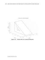
of 40 years is $733,272. The related graph of q(t) duplicates the data listed on the
text screen. The reader may Þnd it interesting to repeat the illustrative calculation
assuming R =11, in which case the saving coefÞcient is greatly reduced to only
$1060.
1.4 Computer Code and Results
A computer code which analyzes the above equations and presents both numerical

and graphical results appears next. First we show the program output, and then
discuss particular aspects of the program.
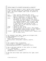
1.4.1 Computer Output
>> finance;
ANALYSIS OF THE SAVE-SPEND PROBLEM BY SOLVING
q’(t)=r*q(t)+[s*(t<=t1)-p*(t>t1)*exp(-a*t1)]*exp(a*t)
where r=R-I, a=A-I, and q(0)=q0
To list parameter definitions enter y
otherwise enter n ? y
INPUT QUANTITIES:
R - annual percent earnings on assets
I - annual percent inflation rate
A - annual percent increase in savings
to offset inflation
r,a - inflation adjusted values of R and I
t1 - saving period (years), 0<t<t1
t2 - payout period (years), t1<t<(t1+t2)
s - saving rate at t=0, ($K). Saving is
© 2003 by CRC Press LLC
expressed as s*exp(a*t), 0<t<t1
p - payout rate at t=t1, ($K). Payout is
expressed as
-p*exp(a*(t-t1)), t1<t<(t1+t2)
q0 - initial savings at t=0, ($K)
q2 - final savings at t=T2=t1+t2, ($K)
OUTPUT QUANTITIES:
q - vector of inflation adjusted savings
values for 0 <= t <= (t1+t2)
t - vector of times (years) corresponding
to the components of q

q1 - value of savings at t=t1, when the
saving period ends
Press return to continue
Input R,A,I (try 11,4,4) ? 8,4,4
Input t1,t2 (try 40,20) ? 40,20
Input q0,s,p,q2 (try 20,5,nan,40) ? 20,nan,50,100
PROGRAM RESULTS
t1 t2 R A I
40.000 20.000 8.000 4.000 4.000
q0 q1 q2 s p
20.000 733.272 100.000 6.417 50.000
>>
© 2003 by CRC Press LLC
0 10 20 30 40 50 60
0
100
200
300
400
500
600
700
800
TOTAL SAVINGS WHEN T1 = 40, T2 = 20, s = 6.4175, p = 50
TIME IN YEARS
TOTAL SAVINGS IN $K
R = 8.000
I = 4.000
A = 4.000
q0 = 20.000

q1 = 733.272
q2 = 100.000
Figure 1.1: Accumulated Assets versus Time
© 2003 by CRC Press LLC
1.4.2 Discussion of the MATLAB Code
Let us examine the following program listing. The line numbers, which are not
part of the actual code, are helpful for discussing particular parts of the program. A
numbered listing can be obtained with the MATLAB command dbtype.
Line Comments
1-2 Three dots . . . are used to continue function Þnance to handle the
long argument list. The output list duplicates some input items to
handle cases involving interactive input.
3-16 Comment lines always begin with the % symbol. At the inter-
active command level in MATLAB, typing help followed by a
function name will print documentation in the Þrst unbroken se-
quence of comments in a function or script Þle.
20-25 The output heading is printed. Note that q”(t) is used to print q’(t)
because special characters such as ’ or % must be repeated.
29-50 Intrinsic function char is used to store descriptions of program
variable in a character matrix.
59 Function nargin checks whether the number of input variables is
zero. If so, data values are read interactively.
68-69 Function inputv reads several variables on the same line.
70-78 While 1, ,end code sequence loops repeatedly to check data in-
put. Break exits to line 80 if data are OK.
85-97 Set multiplier constants to solve for one unknown variable among
q0, s, p, q2.
99-105 Determine time vectors to evaluate the solution. Cases where t1
or t2 are zero require special treatment.
108-112 Intrinsic function isnan is used to identify the variable which was

input as nan.
115-116 User deÞned function savespnd is used to evaluate q(t) and q(t1).
119-127 Program results are printed with a chosen format. The statement
b=inline(’blanks(j)’,’j’) just shortens the name for intrinsic func-
tion blanks.
130-139 Draw the graph along with a title and axis labels.
141-153 Create a label containing data values. Position it on the graph.
154 Turn the grid off and bring the graph to the foreground.
158-176 Function savespnd evaluates q(t). The formula for r=a results
from the limiting form of q(t) as parameter a tends to r.
180-213 Function inputv generalizes the intrinsic function input to read
several variables on the same line. Inputv is used often through-
out this text.
© 2003 by CRC Press LLC
1.4.3 Code for Financial Problem
Program Þnance
1: function [q,t,R,A,I,t1,t2,s,p,q0,q1,q2]=finance
2: (R,A,I,t1,t2,s,p,q0,q2)
3: % [q,t,R,A,I,t1,t2,s,p,q0,q1,q2]=finance
4: % (R,A,I,t1,t2,s,p,q0,q2)
5: %~~~~~~~~~~~~~~~~~~~~~~~~~~~~~~~~~~~~~~~~~~~~~
6: %
7: % This function solves the SAVE-SPEND PROBLEM
8: % where funds earning interest are accumulated
9: % during one period and paid out in a subsequent
10: % period. The value of assets is adjusted to
11: % account for inflation. This problem is
12: % governed by the differential equation
13: % q’(t)=r*q(t)+[s*(t<=t1)
14: % -p*(t>t1)*exp(-a*t1)]*exp(a*t) where

15: % r=R-I, a=A-I and the remaining parameters
16: % are defined below
17:
18:
% User m functions required: inputv, savespnd
19:
20:
disp(’ ’), disp([’ ’,
21: ’ANALYSIS OF THE SAVE-SPEND PROBLEM BY SOLVING’])
22: disp(
23: [’q’’(t)=r*q(t)+[s*(t<=t1)-p*(t>t1)*’,
24: ’exp(-a*t1)]*exp(a*t)’]), disp(
25: ’where r=R-I, a=A-I, and q(0)=q0’), disp(’ ’)
26:
27:
% Create a character variable containing
28: % definitions of input and output quantities
29: explain=char(’INPUT QUANTITIES:’,
30: ’R - annual percent earnings on assets’,
31: ’I - annual percent inflation rate’,
32: ’A - annual percent increase in savings’,
33: ’ to offset inflation’,
34: ’r,a - inflation adjusted values of R and I’,
35: ’t1 - saving period (years), 0<t<t1’,
36: ’t2 - payout period (years), t1<t<(t1+t2)’,
37: ’s - saving rate at t=0, ($K). Saving is’,
38: ’ expressed as s*exp(a*t), 0<t<t1’,
39: ’p - payout rate at t=t1, ($K). Payout is’,
40: ’ expressed as’,
© 2003 by CRC Press LLC

41: ’ -p*exp(a*(t-t1)), t1<t<(t1+t2)’,
42: ’q0 - initial savings at t=0, ($K)’,
43: ’q2 - final savings at t=T2=t1+t2, ($K)’,’ ’,
44: ’OUTPUT QUANTITIES:’,
45: ’q - vector of inflation adjusted savings’,
46: ’ values for 0 <= t <= (t1+t2)’,
47: ’t - vector of times (years) corresponding’,
48: ’ to the components of q’,
49: ’q1 - value of savings at t=t1, when the’,
50: ’ saving period ends’,’ ’);
51:
52:
% NOTE: WHEN R,I,A,T1,T2 ARE KNOWN,THEN FIXING
53: % ANY THREE OF THE VALUES q0,s,p,q2 DETERMINES
54: % THE UNKNOWN VALUE WHICH SHOULD BE GIVEN AS
55: % nan IN THE DATA INPUT.
56:
57:
% Read data interactively when input data is not
58: % passed through the call list
59: if nargin==0
60: disp(’To list parameter definitions enter y’)
61: querry=input(’otherwise enter n ? ’,’s’);
62: if querry==’Y’ | querry==’y’
63: disp(explain); disp(’Press return to continue’)
64: pause, disp(’ ’)
65: end
66:
67:
% Read multiple variables on the same line

68: [R,A,I]=inputv(’Input R,A,I (try 11,4,4) ? ’);
69: [t1,t2]=inputv(’Input t1,t2 (try 40,20) ? ’);
70: while 1
71: [q0,s,p,q2]=inputv(
72: ’Input q0,s,p,q2 (try 20,5,nan,40) ? ’);
73: if sum(isnan([q0,s,p,q2]))==1, break; end
74: fprintf([’\nDATA ERROR. ONE AND ONLY ’,
75: ’ONE VALUE AMONG\n’,’THE PARAMETERS ’,
76: ’q0,s,p,q2 CAN EQUAL nan \n\n’])
77: end
78: end
79:
80:
nt=101; T2=t1+t2; r=(R-I)/100; a=(A-I)/100;
81: c0=exp(r*T2);
82:
83:
% q0,s,p,q2 are related by q2=c0*q0+c1*s+c2*p
84: % Check special case where t1 or t2 are zero
85: if t1==0
© 2003 by CRC Press LLC
86: disp(’ ’), disp(’s is set to zero when t1=0’)
87: s=0; c1=0;
88: else
89: c1=savespnd(T2,t1,0,R,A,I,1,0);
90: end
91:
92:
if t2==0
93: disp(’ ’), disp(’p is set to zero when t2=0’)

94: p=0; c2=0;
95: else
96: c2=savespnd(T2,t1,0,R,A,I,0,1);
97: end
98:
99:
if t1==0 | t2==0
100: t=linspace(0,T2,nt)’;
101: else
102: n1=max(2,fix(t1/T2*nt));
103: n2=max(2,nt-n1)-1;
104: t=[t1/n1*(0:n1),t1+t2/n2*(1:n2)]’;
105: end
106:
107:
% Solve for the unknown parameter
108: if isnan(q0), q0=(q2-s*c1-p*c2)/c0;
109: elseif isnan(s), s=(q2-q0*c0-p*c2)/c1;
110: elseif isnan(p), p=(q2-q0*c0-s*c1)/c2;
111: else, q2=q0*c0+s*c1+p*c2;
112: end
113:
114:
% Compute results for q(t)
115: q=savespnd(t,t1,q0,R,A,I,s,p);
116: q1=savespnd(t1,t1,q0,R,A,I,s,p);
117:
118:
% Print formatted results
119: b=inline(’blanks(j)’,’j’); B=b(3); d=’%8.3f’;

120: u=[d,B,d,B,d,B,d,B,d,’\n’]; disp(’ ’)
121: disp([b(19),’PROGRAM RESULTS’])
122: disp([’ t1 t2 R’,
123: ’ A I’])
124: fprintf(u,t1,t2,R,A,I), disp(’ ’)
125: disp([’ q0 q1 q2’,
126: ’ s p’])
127: fprintf(u,q0,q1,q2,s,p), disp(’ ’), pause(1)
128:
129:
% Show results graphically
130: plot(t,q,’k’)
© 2003 by CRC Press LLC
131: title([’INFLATION ADJUSTED SAVINGS WHEN ’,
132: ’S = ’,num2str(s),’ AND P = ’,num2str(p)]);
133: titl=
134: [’TOTAL SAVINGS WHEN T1 = ’,num2str(t1),
135: ’, T2 = ’,num2str(t2),’, s = ’,num2str(s),
136: ’, p = ’,num2str(p)]; title(titl)
137:
138:
xlabel(’TIME IN YEARS’)
139: ylabel(’TOTAL SAVINGS IN $K’)
140:
141:
% Character label showing data parameters
142: label=char(
143: sprintf(’R = %8.3f’,R),
144: sprintf(’I = %8.3f’,I),
145: sprintf(’A = %8.3f’,A),

146: sprintf(’q0 = %8.3f’,q0),
147: sprintf(’q1 = %8.3f’,q1),
148: sprintf(’q2 = %8.3f’,q2));
149: w=axis; ymin=w(3); dy=w(4)-w(3);
150: xmin=w(1); dx=w(2)-w(1);
151: ytop=ymin+.8*dy; Dy=.065*dy;
152: xlft=xmin+0.04*dx;
153: text(xlft,ytop,label)
154: grid off, shg
155:
156:
%=============================================
157:
158:
function q=savespnd(t,t1,q0,R,A,I,s,p)
159: %
160: % q=savespnd(t,t1,q0,R,A,I,s,p)
161: %~~~~~~~~~~~~~~~~~~~~~~~~~~~~~~~~~~~~~~~~~~~~~
162:
163:
% This function determines q(t) satisfying
164: % q’(t)=r*q+[s*(t<=t1)-p*(t>t1)*
165: % exp(-a*t1)]*exp(a*t), with q(0)=q0,
166: % r=(R-I)/100; a=(A-I)/100
167:
168:
r=(R-I)/100; a=(A-I)/100; c=r-a; T=t-t1;
169: if r~=a
170: q=q0*exp(r*t)+s/c*(exp(r*t)-exp(a*t))
171: -(p+s*exp(a*t1))/c*(T>0).*(

172: exp(r*T)-exp(a*T));
173: else % limiting case as a=>r
174: q=q0*exp(r*t)+s*t.*exp(r*t)
175: -(p+s*exp(r*t1)).*T.*(T>0).*exp(r*T);
© 2003 by CRC Press LLC
176: end
177:
178:
%=============================================
179:
180:
function varargout=inputv(prompt)
181: %
182: % [a1,a2, ,a_nargout]=inputv(prompt)
183: %~~~~~~~~~~~~~~~~~~~~~~~~~~~~~~~~~~~~~~~~~~~~~
184: %
185: % This function reads several values on one
186: % line. The items should be separated by
187: % commas or blanks.
188: %
189: % prompt - A string preceding the
190: % data entry. It is set
191: % to ’ ? ’ if no value of
192: % prompt is given.
193: % a1,a2, ,a_nargout - The output variables
194: % that are created. If
195: % not enough data values
196: % are given following the
197: % prompt, the remaining
198: % undefined values are

199: % set equal to NaN
200: %
201: % A typical function call is:
202: % [A,B,C,D]=inputv(’Enter values of A,B,C,D: ’)
203: %
204: %
205:
206:
if nargin==0, prompt=’ ? ’; end
207: u=input(prompt,’s’); v=eval([’[’,u,’]’]);
208: ni=length(v); no=nargout;
209: varargout=cell(1,no); k=min(ni,no);
210: for j=1:k, varargout{j}=v(j); end
211: if no>ni
212: for j=ni+1:no, varargout{j}=nan; end
213: end
© 2003 by CRC Press LLC
Chapter 2
Elementary Aspects of MATLAB Graphics
2.1 Introduction
MATLAB’s capabilities for plotting curves and surfaces are versatile and easy to
understand. In fact, the effort required to learn MATLAB would be rewarding even
if it were only used to construct plots, save graphic images, and output publication
quality graphs on a laser printer. Numerous help features and well-written demo pro-
grams are included with MATLAB. By executing the demo programs and studying
the relevant code, users can quickly understand the techniques necessary to imple-
ment graphics within their programs. This chapter discusses a few of the graphics
commands. These commands are useful in many applications and do not require
extensive time to master. This next section provides a quick overview of the ba-
sics of using MATLAB’s graphics. The subsequent sections in this chapter present

several additional examples (summarized in the table below) involving interesting
applications which use these graphics primitives.
Example Purpose
Polynomial Inter-
polation
2-D graphics and polynomial interpolation
functions
Conformal 2-D graphics and some aspects of complex
Mapping numbers
Pendulum Motion 2-D graphics animation and ODE solution
Linear Vibration
Model
Animated spring-mass response
String Vibration 2-D and 3-D graphics for a function of form
y(x, t)
Space Curve Ge-
ometry
3-D graphics for a space curve
Intersecting Sur-
faces
3-D graphics and combined surface plots
© 2003 by CRC Press LLC
2.2 Overview of Graphics
The following commands should be executed since they will accelerate the under-
standing of graphics functions, and others, included within MATLAB.
help help discusses use of help command.
help lists categories of help.
help general lists various utility commands.
help more describes how to control output paging.
help diary describes how to save console output to a Þle.

help plotxy describes 2D plot functions.
help plotxyz describes 3D plot functions.
help graphics describes more general graphics features.
help demos lists names of various demo programs.
intro executes the intro program showing MATLAB
commands including fundamental graphics capa-
bilities.
help funfun describes several numerical analysis programs
contained in MATLAB.
type humps lists a function employed in several of the MAT-
LAB demos.
fplotdemo executes program fplotdemo which plots the
function named humps.
help peaks describes a function peaks used to illustrate sur-
face plots.
peaks executes the function peaks to produce an inter-
esting surface plot.
spline2d executes a demo program to draw a curve through
data input interactively.
The example programs can be studied interactively using the type command to list
programs of interest. Library programs can also be inspected and printed using the
MATLAB editor, but care should be taken not to accidentally overwrite the original
library Þles with changes. Furthermore, text output in the command window can be
captured in several ways. Some of these are: (1) Use the mouse to highlight material
of interest. Then use the ”Print Selected” on the Þle menu to send output to the
printer; (2) Use CTRL-C to copy outlined text to the clipboard. Then open a new Þle
and use CTRL-V to paste the text into the new Þle; and (3) Use a diary command
such as diary mysave.doc to begin printing subsequent command window output
into the chosen Þle. This printing can be turned off using diary off. Then the Þle can
be edited, modiÞed, or combined with other text using standard editor commands.

More advanced features of MATLAB graphics, including handle graphics, control
of shading and light sources, creation of movies, etc., exceed the scope of the present
text. Instead we concentrate on using the basic commands listed below and on pro-
ducing simple animations. The advanced graphics can be mastered by studying the
© 2003 by CRC Press LLC