Aerodynamics for engineering students - part 7 docx
Bạn đang xem bản rút gọn của tài liệu. Xem và tải ngay bản đầy đủ của tài liệu tại đây (1.7 MB, 61 trang )
358
Aerodynamics for
Engineering
Students
Fig.
6.47
and integrating gives after substituting for
E;
and
E;
Now,
by
geometry,
and
since
EO
is small,
EO
=
2(t/c),
giving
The lift/drag ratio is a maximum when, by division,
D/L
=
a
+
[;(t/~)~l/a]
is
a minimum, and
this
occurs when
Then
1
c
0.433
=-
a
[;I,,=
-
a2+a2
2a
4
t
t/c
For a
10%
thick section
(LID),,
=
44 at
a
=
6.5"
Moment coefficient and
kcp
Directly from previous work, i.e. taking the moment
of
SL
about the leading edge:
(6.157)
Compressible
flow
359
0.9
-
-
4
8
12
16
20
24
Fig.
8.48
and the centre of pressure coefficient
=
-(CM/CL)
=
0.5 as before.
A
series of results
of tests on supersonic aerofoil sections published by
A.
Ferri* serve to compare with
the theory. The set chosen here is for a symmetrical bi-convex aerofoil section
of
t/c
=
0.1
set in an air flow of Mach number
2.13.
The incidence was varied from
-10" to
28"
and also plotted
on
the graphs of Fig. 6.48 are the theoretical values
of
Eqns (6.156) and (6.157).
Examination of Fig. 6.48 shows the close approximation
of
the theoretical
values to the experimental results. The lift coefficient varies linearly with incidence
but at some slightly smaller value than that predicted.
No
significant reduction in
CL,
as
is
common at high incidences in low-speed tests, was found even with
incidence
>20".
The measured drag values are all slightly higher than predicted which is under-
standable since the theory accounts for wave drag only. The difference between
the two may be attributed to skin-friction drag or, more generally, to the presence
of viscosity and the behaviour of the boundary layer. It is unwise, however, to
expect the excellent agreement of these particular results to extend to more general
aerofoil sections
-
or indeed to other Mach numbers for the same section, as
severe limitations on the use of the theory appear at extreme Mach numbers.
Nevertheless, these and other published data amply justify the continued use of
the theory.
*
A.
Ferri, Experimental results with
aerofoils
tested
in
the high-speed tunnel
at
Guidornia,
Atti
Guidornia,
No.
17, September 1939.
360
Aerodynamics
for
Engineering
Students
General aerofoil section
Retaining the major assumptions of the theory that aerofoil sections must be
slender and sharp-edged permits the overall aerodynamic properties to be assessed
as the
sum
of contributions due to thickness, camber and incidence. From previous
sections it
is
known that the local pressure at any point on the surface is due to the
magnitude and sense of the angular deflection of the flow from the free-stream
direction. This deflection in turn can be resolved into components arising from the
separate geometric quantities of the section, i.e. from the thickness, camber and
chord incidence.
The principle is shown figuratively in the sketch, Fig.
6.49,
where the pressure
p
acting on the aerofoil at a point where the flow deflection from the free stream is
E
may be considered as the
sum
ofpt
+
pc $-pa.
If, as is more convenient, the pressure
coefficient is considered, care must be taken to evaluate the
sum
algebraically. With
the notation shown in Fig.
6.49;
CP
=
CPt
+
CPC
+
Ch
(6.158)
or
(6.159)
Lvt
The lift coefficient due to the element of surface is
SX
-2
(Et+Ec+E,)-
sc
-
C
L-dFT
which is made up of terms due to thickness, camber and incidence.
On
integrating
round the surface of the aerofoil the contributions due to thickness and camber
vanish leaving only that due
to
incidence. This can be easily shown by isolating the
contribution due to camber, say, for the upper surface. From Eqn
(6.148)
D
Symmetrical
+
\
section
r-
contributing
thickness
in
Incidence
contribution
Fig.
6.49
Compressible
flow
361
but
~c~cdx=~~(~)cdx=~cdyc=
k];=O
Therefore
CLCamber
=
0
Similar treatment of the lower surface gives the same result, as does consideration of
the contribution to the lift due to the thickness.
This result is also borne out by the values of
CL
found in the previous examples, Le.
Now (upper surface)
=
-a
and (lower surface)
=
+a
4a
CL
=
m
(6.160)
Drug
(wave)
The drag coefficient due to the element of surface shown in Fig. 6.49 is
which,
on
putting
E
=
+ +
E~
etc., becomes
On integrating this expression round the contour to find the overall drag, only the
integration of the squared terms contributes, since integration of other products
vanishes for the same reason as given above for the development leading to
Eqn
(6.160). Thus
(6.161)
Now
2
~idx
=
4a2c
f
362
Aerodynamics
for
Engineering Students
and for a particular section
and
2
E:&=
kcP2c
!
so
that for a given aerofoil profile the drag coefficient becomes in general
(6.16
1
a)
where
t/c
and
P
are the thickness chord ratio and camber, respectively, and
kt, k,
are
geometric constants.
Lift/wave drag
ratio
It follows from
Eqns
(6.160)
and
(6.161)
that
D
kt(t/c)’
+
ktP2
-=a+
4a
L
which is a minimum when
kt(t/C)2
+
kcP2
4
a=
Moment coefficient and centre
of
pressure coefjcient
Once again the moment about
the leading edge is generated from the normal contribution and for the general
element of surface x from the leading edge
6cM=-(
2
)-&-
x dx
JmC
c
x dx
CM
=
h?=-l
cc
Now
is zero for the general symmetrical thickness, since the pressure distribution due to
the section (which, by definition, is symmetrical about the chord) provides neither lift
nor moment, i.e. the net lift at any chordwise station is zero. However, the effect of
camber is not zero in general, although the overall lift is zero (since the integral
of
the
slope is zero) and the influence of camber is to exert a pitching moment that is
negative (nose down for positive camber), i.e. concave downwards. Thus
Compressible
flow
363
The centre of pressure coefficient follows from
1
and this is
no
longer independent of incidence, although it is still independent of
Mach number.
Aerofoil section made
up
of
unequal circular arcs
A
convenient aerofoil section to consider as a first example is the biconvex aerofoil
used by Stanton* in some early work
on
aerofoils at speeds near the speed of sound.
In
his experimental work he used a conventional, i.e. round-nosed, aerofoil
(RAF
31a) in addition to the biconvex sharp-edged section at subsonic as well as supersonic
speeds, but the only results used for comparison here will be those for the biconvex
section at the supersonic speed
M
=
1.12.
Example
6.11
Made up of two unequal circular arcs a profile has the dimensions
shown in Fig.
6.50.
The exercise here is to compare the values of lift, drag, moment
and centre of pressure coefficients found by Stanton* with those predicted by Ackeret's
theory. From the geometric data given, the tangent angles at leading and trailing edges
are 16"
=
0.28 radians and
7"
=
0.12radians for upper and lower surfaces respectively.
Then, measuring
x
from the leading edge, the local deflections from the free-stream direction are
~~~0.28 1-2-
-a
(
:>
and
&L=0.12 1-2-
+a
(
:>
for upper and lower surfaces respectively.
M
=
I
.72
Fig.
6.50
Stanton's biconvex aerofoil section
t/c
=
0.1
*
T.E.
Stanton,
A
high-speed wind
channel for
tests
on
aerofoils,
ARCR
and
M,
1130,
January
1928.
364
Aerodynamics
for
Engineering Students
L$t coefficient
4a
CL
=-
drn
For
M
=
1.72
CL
=
2.86a
Drag (wave) coefficient
/'
[
(0.28
(1
-
$)
-
a)2+(0.12(1- 2q
+
a)
2
]
dx
cD=cm
0
C
(4aZ
+
0.0619)
m
CD
=
For
M
=
1.72
(as
in
Stanton's
case),
Co
=
2.86~~'
+
0.044
Moment coefficient (about leading edge)
or
2
CM,
=
dm
[a
+
0.02711
For
M
=
1.72
=
1.43~~
+
0.039
Centre-of-pressure coefficient
-CM~
2a
+
0.054
ke=
-
CL
4a
0.5
+
0.0135
a
kcp
=
L$t/drag ratio
4a
L
-
m=
a
D
4a2
+
0.0619
CY'
-
0.0155
dm
This
is
a
maximum
when
a
=
dm
=
0.125rads.
=
8.4"
giving
(LID),
=
4.05.
Compressible
flow
365
0.4
c, 0.2
t//
/
&served
Ca,
/-
2.5 5.0
7.5
a0
Ob
1
I
I
L
I
/
/I
I
I I
0
2.5
5.0
7.5
a0
1
0.15
0.05
I
I
I
I
o1
2.5
5.0
7.5
G
llo
1,
0
I
2.5 5.0 7.5
I
ao
t
I
Incidence degrees
0
2.5 5.0 7.5
CL
calculated
observed
CD
calculated
observed
-
CM
calculated
observed
kCP
calculated
observed
LID
calculated
observed
0
0.1 25
-0.064
0.096
0-044
0.0495
0.052 0.054
0.039 0.101
-0.002 0.068
m
0.81
0.03 0-69
0
2.5
-1.2
1
-8
0.25
0.203
0.066
0.070
0-1 64
0.1 14
0.65
0.54
3.8
2.9
0-375
0.342
0.093
0-093
0.226
0.1 78
0.60
0.49
4.0
3.5
Fig. 6.51
It will be noted again that the calculated and observed values are close in shape but the latter
are lower in value, Fig. 6.51. The differences between theory and experiment are probably
explained by the fact that viscous drag is neglected in the theory.
Double
wedge
aerofoil
section
Example
6.12
Using Ackeret's theory obtain expressions for the lift and drag coefficients
of
the cambered double-wedge aerofoil shown in Fig. 6.52. Hence show that the minimum
lift-drag ratio for the uncambered doublewedge aerofoil is
fi
times that for a cambered
one with
h
=
t/2. Sketch the flow patterns and pressure distributions around both aerofoils at
the incidence for
(L/D),,,ax.
(u
of
L)
366
Aetudynamics
for
Engineering Students
Fig.
6.52
Lift
Previous
work, Eqn (6.160) has shown that
Drag (wave)
From
Eqn
(6.161) on the general aerofoil
Here, as before:
2
&;-=4azC
f:
For
the
given geometry
i.e. one equal contribution from each of four flat surfaces, and
Le. one equal contribution from each of four flat surfaces. Therefore
Lift-drag ratio
L
Cr
a
I
D=G=
[
a’+
(a’
-
+4
(3’1
-
For the uncambered aerofoil
h
=
0:
For
the cambered section, given
h
=
t/c:
hprsssible
flow
367
No
camber
Upper surface
Rear
f
a=
for
[$Im
c
Lower
surface
Fig.
6.53
Flow
patterns and pressure distributions around both aerofoils at incidence
of
[L/D],,,
6.8.4
Other aspects
of
supersonic wings
The shock-expansion approximation
The supersonic linearized theory has the advantage of giving relatively simple for-
mulae for the aerodynamic characteristics of aerofoils. However,
as
shown below
in
Example
6.13
the exact pressure distribution can
be
readily found for a double-wedge
aerofoil. Hence the coefficients of lift and drag can
be
obtained.
Fixample
6.13 Consider a symmetrical double-wedge aerofoil at zero incidence, similar
in
shape to that in Fig.
6.44
above, except that the semi-wedge angle
EO
=
10". Sketch the wave
pattern for
M,
=
2.0, calculate the Mach number and pressure
on
each face of the aerofoil,
and hence determine
Co.
Compare the results
with
those obtained using the linear theory.
Assume the free-stream stagnation pressure,
porn
=
1
bar.
The wave pattern
is
sketched
in
Fig. 6.54a. The flow properties in the various regions can
be
obtained using isentropic flow and oblique shock tables.*
In
region
1
M
=
M,
=
2.0 and
ph
=
1 bar. From the isentropic flow tables
pol/pl
=
7.83 leading to
p1
=
0.1277 bar.
In
region 2 the oblique shock-wave tables give
p2/p1
=
1.7084 (leading to
p2
=
0.2182 bar),
M2
=
1.6395 and shock angle
=
39.33". Therefore
(0.2182/0.1277)
-
1
=
0.253
- -
0.5
x
1.4
x
22
e.g.
E.L.
Houghton
and
A.E.
Brock,
Tables
for
the
Compressible
Flow
of
Dry
Air,
3rd Edn., Edward
Arnold,
1975.
368
Aerodynamics
for
Engineering Students
Oblique
shock
waves
M=
2.0
(a)
Stand-off
bow
shock
wave
\
Fig.
6.54
(Using the linear
theory,
Eqn
(6.145)
gives
In
order
to
continue the
calculation
into region
3
it is
first
necessary
to
determine the Prandtl-Meyer
angle and
stagnation
pressure
in
region
2.
These
can
be
obtained
as
follows
using
the isentropic
flow
tables:p&
=
4.516
givingpm
=
4.516
x
0.2182
=
0.9853
bar; and
Machangle,
p~
=
37.57"
and
Prandtl-Meyer angle,
v2
=
16.01'.
Between
regions
2
and
3
the
flow
expands isentropically
through
20"
so
v3
=
v2
+
20"
=
36.01'.
From
the isentropic
flow
tables
this
value
of
v3
corresponds to
M3
=
2.374,
p3
=
24.9"
and
Compressible
flow
369
p03/p3
=
14.03. Since the expansion is isentropic
po3
=
poz
=
0.9853 bar
so
that
p3
=
0.9853/14.03
=
0.0702 bar.
Thus
=
-0.161
(0.0702/0.1277)
-
1
cp3=
0.7
x
22
(Using the linear theory, Eqn (6.145) gives
2E -2
x
(lO?T/180)
c-
=
-0.202)
p3-4T5T=
dK-i
There is an oblique shock wave
between
regions
3 and 4. The oblique shock tables give
p4/p3
=
1.823 and
M4
=
1.976 givingp4
=
1.823
x
0.0702
=
0.128 bar and a shock angle of 33.5".
The drag per unit span acting
on
the aerofoil is given by resolving the pressure forces,
so
that
so
CD
=
(Cpz
-
Cp3) tan( 100)
=
0.0703
(Using the linear theory, Eqn (6.151) with
o
=
0
gives
It can be
seen
from the calculations above that, although the linear theory does not approx-
imate the value of
C,
very accurately, it does yield an accurate estimate of
CD.
When
M,
=
1.3 it can be seen from the oblique shock tables that the maximum compres-
sion angle is less than 10".
This
implies that in this case the
flow
can only negotiate the leading
edge by being compressed through a shock wave that stands
off
from the leading edge and is
normal to the flow where it intersects the extension of the chord line. This leads to a region of
subsonic
flow
being formed between the stand-off shock wave and the leading edge. The
corresponding
flow
pattern is sketched in Fig. 6.54b.
A
similar
procedure to that in Example
6.13
can be followed for aerofoils with curved
profiles.
In
this case, though, the procedure becomes approximate because it ignores
the effect of the Mach waves reflected from the bow shock wave
-
see
Fig.
6.55.
The
so-called shock-expansion approximation is made clearer by the example given below.
Example
6.14
Consider a biconvex aerofoil at zero incidence in supersonic flow at
M,
=
2,
similar in shape to that shown in Fig. 6.46 above
so
that, as before, the shape of the upper
surface is given by
y
=
XE~
1
-
-
giving local flow angle
e(=
E)
=
arc tan
(3
Bow
shock
wave
Reflected
Mach wave
Fig.
6.55
370
Aerodynamics
for
Engineering
Students
Calculate the pressure and Mach number along the surface as functions of
x/c
for the case of
EO
=
0.2.
Compare with the results obtained with linear theory. Take the freestream stagnation
pressure
to
be
1
bar.
Region
1
as in Example
6.13,
i.e.
M1
=
2.0,
pol
=
1
bar and
p1
=
0.1277
bar
At
x
=
0
e
=
arctan(0.2)
=
11.31'.
Hence initially the flow is turned by the bow shock
through an angle of
11.31",
so
using the oblique shock tables gives
p2/p1
=
1.827
and
M2
=
1.59.
Thuspz
=
1.827
x
0.1277
=
0.233
bar. From the isentropic flow tables it
is
found
that M2
=
1.59
corresponds topo2/p2
=
4.193
givingpo2
=
0.977
bar.
Thereafter the pressures and Mach numbers around the surface
can
be obtained using the
isentropic flow tables
as
shown in the table below.
f
tan0
0.0
0.2
0.1 0.16
0.2 0.12
0.3
0.08
0.5
0.0
0.7
-0.08
0.8 -0.12
0.9 -0.16
1.0 -0.20
e
11.31"
9.09"
6.84"
4.57"
0.0
-4.57"
-6.84"
-9.09"
-11.31"
ne
0"
2.22"
4.47"
6.74"
11.31'
15.88"
18.15"
20.40"
22.62"
V
14.54"
16.76"
19.01'
21.28"
25.85"
30.42'
32.69"
34.94"
37.16"
M
1.59
1.666
1.742
1.820
1.983
2.153
2.240
2.330
2.421
h
P
4.193
4.695
5.265
5.930
7.626
9.938
11.385
13.104
15.102
0.233
0.208
0.186
0.165
0.128
0.098
0.086
0.075
0.065
CP
0.294
0.225
0.163
0.104
0.0008
-0.0831
-0.1166
-0.1474
-0.1754
WP)li7l
0.228
0.183
0.138
0.092
0
-0.098
-0.138
-0.183
-0.228
Wings
of
finite span
When the component of the free-stream velocity perpendicular to the leading edge
is
greater than the local speed of sound the wing is said to have
a
supersonic leading
edge.
In
this case, as illustrated in Fig.
6.56,
there is two-dimensional supersonic flow
over much
of
the wing. This flow can be calculated using supersonic aerofoil theory.
For the rectangular wing shown in Fig.
6.56
the presence of a wing-tip can only be
communicated within the Mach cone apex which is located
at
the wing-tip. The same
consideration would apply
to
any inboard three-dimensional effects, such as the
'kink' at the centre-line of a swept-back wing.
The opposite case is when the component
of
free-stream velocity perpendicular to
the leading edge is less than the local speed
of
sound and the term
subsonic leading
edge
is
used.
A
typical example is the swept-back wing shown in Fig.
6.57.
In
this
case
the Mach cone generated by the leading edge of the centre section subtends the whole
wing. This implies that the leading edge of the outboard portions of the wing
influences the oncoming flow just as for subsonic flow. Wings having finite thickness
and incidence actually generate a shock cone, rather than a Mach cone, as shown
in
Mach cone
Tip
effects
Fig.
6.56
A
typical wing with
a
supersonic leading edge
Compressible
flow
371
Fig,
6.57
A
wing with
a
subsonic
leading edge
Fig.
6.58
Fig. 6.58. Additional shocks are generated by other points on the leading edge and
the associated shock angles will tend to increase because each successive shock wave
leads to a reduction in the Mach number. These shock waves progressively decelerate
the flow,
so
that at some section, such as
AA',
the flow approaching the leading edge
will be subsonic. Thus subsonic wing sections would be used over most of the wing.
Wings with subsonic leading edges have lower wave drag than those with super-
sonic ones. Consequently highly swept wings, e.g. slender deltas, are the preferred
configuration at supersonic speeds. On the other hand swept wings with supersonic
leading edges tend to have a greater wave drag than straight wings.
Computational
methods
Computational methods for compressible flows, particularly transonic flow over
wings, have been the subject of a very considerable research effort over the past three
decades. Substantial progress has been made, although much still remains to be done.
A discussion of these methods is beyond the scope of the present book, save to note
that for the linearized compressible potential flow Eqn (6.1 18) panel methods (see
Sections
3.5,
4.10
and 5.8) have been developed for both subsonic and supersonic
flow. These can be used to obtain approximate numerical solutions in cases with
exceedingly complex geometries. A review of the computational methods developed
for the full inviscid and viscous equations of motion is given by Jameson.*
*A. Jameson, 'Full-Potential, Euler and Navier-Stokes Schemes',
in
Applied Computational Aerodynamics,
Vol.
125
of
Prog. in Astronautics and Aeronautics
(ed.
By
P.A.
Henne),
39-88
(1990),
AIM
New
York.
372
Aerodynamics
for
Engineering Students
Exercises
1
A convergentdivergent duct has a maximum diameter of 15Omm and a pitot-
static tube is placed in the throat of the duct. Neglecting the effect of the Pitot-static
tube
on the flow, estimate the throat diameter under the following conditions:
(i) air at the maximum section is of standard pressure and density, pressure differ-
(ii) pressure and temperature in the maximum section are 101 300
N
m-2
and 100 "C
(Answer:
(i) 123 mm;
(ii)
66.5
mm)
ence across the Pitot-static tube
=
127 mm water;
respectively, pressure difference across Pitot-static tube
=
127
mm
mercury.
2
In
the wing-flow method of transonic research an aeroplane dives at a Mach
number of 0.87 at a height where the pressure and temperature are 46 500NmP2
and -24.6"C respectively. At the position of the model the pressure coefficient is
-0.5.
Calculate the speed, Mach number,
0.7~
M2,
and the kinematic viscosity of the
flow past the model.
(Answer:
344m
s-';
M
=
1.133;
0.7pM2
=
30 XOON m-2;
v
=
2.64
x
10-3m2s-')
3
What would be the indicated air speed and the true air speed of the aeroplane
in
Exercise
2,
assuming the air-speed indicator to be calibrated on the assumption of
incompressible flow in standard conditions, and to have no instrument errors?
(Answer:
TAS
=
274m
s-l;
IAS
=
219m
s-')
4
On
the basis of Bernoulli's equation, discuss the assumption that the compressi-
bility of air may be neglected for low subsonic speeds.
A symmetric aerofoil at zero lift has a maximum velocity which is 10% greater
than
the free-stream velocity. This maximum increases at the rate of 7% of the free-
stream velocity for each degree of incidence. What is the free-stream velocity at which
compressibility effects begins to become important (i.e. the error
in
pressure
coefficient exceeds 2%) on the aerofoil surface when the incidence is
5"?
(Answer:
Approximately 70m
s-')
(U
of
L)
5
A closed-return type of wind-tunnel of large contraction ratio has air at standard
conditions of temperature and pressure in the settling chamber upstream of the
contraction to the working section. Assuming isentropic compressible flow in the
tunnel estimate the speed in the working section where the Mach number is 0.75.
Take the ratio of specific heats for air as
y
=
1.4.
(Answer:
242 m
s-')
(U
of
L)
Viscous
flow
and
boundary layers*
7.1 Introduction
In the other chapters of this
book,
the effects of viscosity, which
is
an inherent
property
of
any real fluid, have, in the main, been ignored. At first sight, it would
seem to be a waste of time to study inviscid fluid flow when all practical fluid
*
This chapter is concerned mainly with incompressible flows. However, the general arguments developed
are also applicable to compressible flows.
374
Aerodynamics
for
Engineering
Students
Effects
of
viscosity negligible
in regions not in close proximity
to the body
Regions where viscous action predominates
t
._
9
Wake
-e
0
-
h
Fig.
7.1
problems involve viscous action. The purpose behind this study by engineers dates
back to the beginning of the previous century
(1904)
when Prandtl conceived the idea
of the
boundary
layer.
In order to appreciate this concept, consider the flow of a fluid past a body of
reasonably slender
form
(Fig.
7.1).
In aerodynamics, almost invariably, the fluid
viscosity is relatively small (i.e. the Reynolds number is high); so that, unless the
transverse velocity gradients are appreciable, the shearing stresses developed [given
by Newton’s equation
I-
=
p(au/dy)
(see, for example, Section
1.2.6
and Eqn
(2.86))]
will be very small. Studies of flows, such as that indicated in Fig.
7.1,
show that the
transverse velocity gradients are usually negligibly small throughout the flow field
except for thin layers of fluid immediately adjacent to the solid boundaries. Within
these boundary layers, however, large shearing velocities are produced with conse-
quent shearing stresses of appreciable magnitude.
Consideration of the intermolecular forces between solids and fluids leads to the
assumption that at the boundary between a solid and a fluid (other than a rarefied
gas) there is a condition of no slip. In other words, the relative velocity of the fluid
tangential to the surface is everywhere zero. Since the mainstream velocity at a small
distance from the surface may be considerable, it is evident that appreciable shearing
velocity gradients may exist within this boundary region.
Prandtl pointed out that these boundary layers were usually very thin, provided that
the body was of streamline form, at a moderate angle of incidence to the flow and that
the flow Reynolds number was sufficiently large;
so
that, as a first approximation, their
presence might be ignored in order to estimate the pressure field produced about the
body. For aerofoil shapes, this pressure field is, in fact, only slightly modified by the
boundary-layer flow, since almost the entire lifting force is produced by normal
pressures at the aerofoil surface, it is possible to develop theories for the evaluation
of the lift force by consideration of the flow field outside the boundary layers, where
the flow is essentially inviscid in behaviour. Herein lies the importance of the inviscid
flow methods considered previously.
As
has been noted
in
Section
4.1,
however, no
drag force, other than induced drag, ever results from these theories. The drag force is
mainly due to shearing stresses at the body surface (see Section
1.5.5)
and it is in the
estimation of these that the study of boundary-layer behaviour is essential.
The enormous simplification in the study of the whole problem, which follows
from Prandtl’s boundary-layer concept, is that the equations of viscous motion need
Viscous
flow
and boundary layers
375
be considered only in the limited regions of the boundary layers, where appreciable
simplifying assumptions can reasonably be made. This was the major single impetus
to the rapid advance in aerodynamic theory that took place in the first half of the
twentieth century. However, in spite of this simplification, the prediction of boundary-
layer behaviour is by no means simple. Modern methods of computational fluid
dynamics provide powerful tools for predicting boundary-layer behaviour. However,
these methods are only accessible to specialists; it still remains essential to study
boundary layers in a more fundamental way to gain insight into their behaviour and
influence on the flow field as a whole. To begin with, we will consider the general
physical behaviour of boundary layers.
7.2
The
development
of
the
boundary
layer
For the flow around a body with a sharp leading edge, the boundary layer
on
any
surface will grow from zero thickness at the leading edge
of
the body. For a typical
aerofoil shape, with a bluff nose, boundary layers will develop on top and bottom
surfaces from the front stagnation point, but will not have zero thickness there (see
Section
2.10.3).
On proceeding downstream along
a
surface, large shearing gradients and stresses
will develop adjacent to the surface because of the relatively large velocities in the
mainstream and the condition of no slip at the surface. This shearing action is
greatest at the body surface and retards the layers of fluid immediately adjacent to
the surface. These layers, since they are now moving more slowly than those above
them, will then influence the latter and
so
retard them. In this way, as the fluid near
the surface passes downstream, the retarding action penetrates farther and farther
away from the surface and the boundary layer of retarded or ‘tired’ fluid grows in
thickness.
7.2.1
Velocity profile
Further thought about the thickening process
will
make it evident that the increase in
velocity that takes place along a normal to the surface must be continuous. Let
y
be
the perpendicular distance from the surface at any point and let
u
be the correspond-
ing velocity parallel to the surface. If
u
were to increase discontinuously with
y
at any
point, then at that point
au/ay
would be infinite. This would imply an infinite
shearing stress [since the shear stress
T
=
p(au/dy)]
which is obviously untenable.
Consider again a small element of fluid (Fig.
7.2)
of unit depth normal to the flow
plane, having a unit length in the direction of motion and a thickness
Sy
normal to
the flow direction. The shearing stress on the lower face AB will be
T
=
p(au/ay)
while that
on
the upper face
CD
will be
T
+
(a
~/by)Sy,
in the directions shown,
assuming
u
to increase with
y.
Thus the resultant shearing force in the x-direction will
be
[T
+
(a
~/dy)Sy]
-
T
=
(a
~/dy)Sy
(since the area parallel to the x-direction is unity)
but
T
=
p(du/dy)
so
that the net shear force on the element
=
p(a2u/ay2)6y.
Unless
p
be zero, it follows that
a2u/ay2
cannot be infinite and therefore the rate of change of
the velocity gradient in the boundary layer must also be continuous.
Also shown in Fig.
7.2
are the streamwise pressure forces acting on the fluid
element. It can be seen that the net pressure force is -(dp/dx)Sx. Actually, owing
to the very small total thickness of the boundary layer, the pressure hardly varies at
all normal to the surface. Consequently, the net transverse pressure force is zero to
a
very good approximation and Fig.
7.2
contains all the significant fluid forces. The
376
Aerodynamics
for
Engineering Students
YA
Fig.
7.2
effects
of
streamwise pressure change are discussed in Section 7.2.6 below. At this
stage it is assumed that
aplax
=
0.
If the velocity
u
is
plotted against the distance
y
it is now clear that a smooth curve
of
the general form shown in Fig. 7.3a must develop (see also Fig. 7.11). Note that at
the surface the curve is not tangential to the
u
axis
as
this
would imply an infinite
gradient
au/ay,
and therefore
an
infinite shearing stress, at the surface. It is also
evident that as the shearing gradient decreases, the retarding action decreases,
so
that
U
-I
U
(a
1
(b)
4
Fig.
7.3
Viscous
flow
and boundary layers
377
at some distance from the surface, when
&lay
becomes very small, the shear stress
becomes negligible, although theoretically a small gradient must exist out to
y
=
m.
7.2.2 Bou ndary-layer thickness
In order to make the idea
of
a boundary layer realistic, an arbitrary decision must be
made as to its extent and the usual convention is that the boundary layer extends to
a distance
5
from the surface such that the velocity
u
at that distance is 99% of the local
mainstream velocity
U,
that would exist at the surface in the absence of the boundary
layer. Thus
6
is the physical thickness of the boundary layer
so
far
as it needs to be
considered and when defined specifically as above it is usually designated the 99%, or
general, thickness. Further thickness definitions are given in Section 7.3.2.
7.2.3 Non-dimensional profile
In order to compare boundary-layer profiles of different thickness, it is convenient to
express the profile shape non-dimensionally. This may be done by writing
ii
=
u/U,
and
J
=
y/S
so
that the profile shape is given by
U
=
f(
7).
Over the range
y
=
0
to
y
=
5,
the velocity parameter
ii
varies from
0
to 0.99. For convenience when using
ii
values as integration limits, negligible error is introduced by using
ii
=
1.0
at the
outer boundary, and considerable arithmetical simplification is achieved. The vel-
ocity profile is then plotted as in Fig. 7.3b.
7.2.4 Laminar and turbulent flows
Closer experimental study of boundary-layer flows discloses that, like flows in pipes,
there are two different regimes which can exist: laminar flow and turbulent flow. In
luminarfZow,
the layers of fluid slide smoothly over one another and there is little
interchange of fluid mass between adjacent layers. The shearing tractions that develop
due to the velocity gradients are thus due entirely to the viscosity
of
the fluid, i.e. the
momentum exchanges between adjacent layers are on a molecular scale only.
In
turbulent
flow
considerable seemingly random motion exists, in the form
of
velocity fluctuations both along the mean direction of flow and perpendicular to it.
As
a result of the latter there are appreciable transports of mass between adjacent
layers. Owing to these fluctuations the velocity profile varies with time. However,
a time-averaged,
or
mean, velocity profile can be defined.
As
there is a mean velocity
gradient in the flow, there will be corresponding interchanges of streamwise momen-
tum between the adjacent layers that will result in shearing stresses between them.
These shearing stresses may well be
of
much greater magnitude than those that
develop as the result
of
purely viscous action, and the velocity profile shape in
a turbulent boundary layer is very largely controlled by these
Reynolds
stresses
(see
Section 7.9), as they are termed.
As
a consequence of the essential differences between laminar and turbulent flow
shearing stresses, the velocity profiles that exist in the two types of layer are also
different. Figure 7.4 shows a typical laminar-layer profile and a typical turbulent-
layer profile plotted to the same non-dimensional scale. These profiles are typical of
those on a flat plate where there is no streamwise pressure gradient.
In the laminar boundary layer, energy from the mainstream is transmitted towards
the slower-moving fluid near the surface through the medium
of
viscosity alone and
only a relatively small penetration results. Consequently, an appreciable proportion
of the boundary-layer flow has a considerably reduced velocity. Throughout the
378
Aerodynamics
for
Engineering
Students
Fig.
7.4
boundary layer, the shearing stress
T
is given by
T
=
p(aU/dy) and the wall shearing
stress is thus
rw
=
p(d~/dy),=~
=
p(du/dy),(say).
In the turbulent boundary layer, as has already been noted, large Reynolds stresses
are set
up
owing to mass interchanges in a direction perpendicular to the surface,
so
that energy from the mainstream may easily penetrate to fluid layers quite close to
the surface.
This
results in the turbulent boundary away from the immediate influ-
ence of the wall having a velocity that is not much less than that of the mainstream.
However, in layers that are very close to the surface (at this stage of the discussion
considered smooth) the velocity fluctuations perpendicular to the wall are evidently
damped out,
so
that in
a
very limited region immediately adjacent to the surface, the
flow approximates to purely viscous flow.
In this
viscous
sublayer the shearing action becomes, once again, purely viscous and
the velocity falls very sharply, and almost linearly, within it, to zero at the surface.
Since, at the surface, the wall shearing stress now depends on viscosity only, i.e.
rw
=
p(du/dy),, it will be clear that the surface friction stress under
a
turbulent layer
will be far greater than that under a laminar layer of the same thickness, since
(du/dy), is much greater. It should be noted, however, that the viscous shear-stress
relation is only employed in the viscous sublayer very close to the surface and not
throughout the turbulent boundary layer.
It
is clear, from the preceding discussion, that the
viscous
shearing stress at the surface,
and thus the surface friction stress, depends only on the slope of the velocity profile at the
surface, whatever the boundary-layer type,
so
that accurate estimation of the profile,
in
either case,
will
enable correct predictions of skin-friction drag to be made.
7.2.5
Growth
along
a
flat
surface
If the boundary layer that develops on the surface of
a
flat plate held edgeways on to the
free stream is studied, it is found that, in general, a laminar boundary layer starts to
Viscous
flow
and
boundary
layers
379
Wake
Transit ion
Turbulent
I
region
\
-T
r-
2
-
Fig.
7.5
Note: Scale normal
to
surface
of
plate
is
greatly exaggerated
develop from the leading edge. This laminar boundary layer grows in thickness, in
accordance with the argument of Section
7.2,
from zero at the leading edge to some
point on the surface where a rapid transition to turbulence occurs (see Fig.
7.29).
This
transition is accompanied by a corresponding rapid thickening of the layer. Beyond this
transition region, the turbulent boundary layer then continues to thicken steadily as it
proceeds towards the trailing edge. Because of the greater shear stresses within the
turbulent boundary layer its thickness is greater than for a laminar one. But, away from
the immediate vicinity of the transition region, the actual rate of growth along the plate
is
lower for turbulent boundary layers than for laminar ones.
At
the trailing edge the
boundary layer joins with the one from the other surface to form a wake of retarded
velocity which
also
tends to thicken slowly as it flows away downstream (see Fig.
7.5).
On a flat plate, the laminar profile has a constant shape at each point along
the surface, although of course the thickness changes,
so
that one non-dimensional
relationship for
ii
=f(v)
is sufficient (see Section
7.3.4).
A
similar argument applies
to a reasonable approximation to the turbulent layer. This constancy of profile
shape means that flat-plate boundary-layer studies enjoy a major simplification and
much work has been undertaken to study them both theoretically and experimentally.
However, in most aerodynamic problems, the surface
is
usually that of a stream-
line form such as a wing or fuselage. The major difference, affecting the boundary-
layer flow in these cases, is that the mainstream velocity and hence the pressure in
a streamwise direction is
no
longer constant. The effect of a pressure gradient along the
flow can be discussed purely qualitatively initially in order to ascertain how the
boundary layer is likely to react.
7.2.6
Effects
of
an external pressure gradient
In the previous section, it was noted that in most practical aerodynamic applications
the mainstream velocity and pressure change in the streamwise direction. This has
a profound effect on the development of the boundary layer. It can be seen from
Fig.
7.2
that the net streamwise force acting on a small fluid element within the
boundary layer is
87
ap
-&y
&x
ay
ax
When the pressure decreases (and, correspondingly, the velocity along the edge of
the boundary layer increases) with passage along the surface the
external
pressure
380
Aerodynamics
for
Engineering Students
1.0-
-
Flat
plate
Favourable pressure gradient
0.8-
0.6
-
'\
0.4
-
0.2
-
0
-0.2
0
0.2
0.4
0.6
0.8
1.0
-
U
Fig.
7.6
Effect
of
external pressure gradient on the velocity profile in the boundary layer
gradient is said to be
favourable.
This is because
dpldx
<
0
so,
noting that
&-lay
<
0,
it can be seen that the streamwise pressure forces help to counter the effects, dis-
cussed earlier, of the shearing action and shear stress at the wall. Consequently, the
flow is not decelerated
so
markedly at the wall, leading to a fuller velocity profile
(see Fig.
7.6),
and the boundary layer grows more slowly along the surface than for
a flat plate.
The converse case is when the pressure increases and mainstream velocity
decreases along the surface. The external pressure gradient
is
now said to be
unfavourable
or
adverse.
This is because the pressure forces now reinforce the effects
of the shearing action and shear stress at the wall. Consequently, the flow decelerates
more markedly near the wall and the boundary layer grows more rapidly than in the
case of the flat plate. Under these circumstances the velocity profile is much less
full than for a flat plate and develops a point
of
inflexion (see Fig.
7.6).
In fact, as
indicated in Fig.
7.6,
if
the adverse pressure gradient is sufficiently strong or pro-
longed, the flow near the wall is
so
greatly decelerated that it begins to reverse
direction. Flow reversal indicates that the boundary layer has
separated
from the
surface. Boundary-layer separation can have profound consequences for the whole
flow field and is discussed in more detail in Section
7.4.
7.3
The boundary-layer equations
To
fix ideas it is helpful to think about the flow over a flat plate. This is a particularly
simple flow, although like much else in aerodynamics the more one studies the details
the less simple it becomes. If we consider the case
of
infinite Reynolds number,
Viscous
flow
and
boundary
layers
381
i.e. ignore viscous effects completely, the flow becomes exceedingly simple. The stream-
lines are everywhere parallel to the flat plate and the velocity uniform and equal to
U,,
the value in the free stream infinitely far from the plate. There would, of course,
be no drag, since the shear stress at the wall would be equivalently zero. (This is
a special case of d'Alembert's paradox that states that no force is generated by irrota-
tional flow around any body irrespective
of
its shape.) Experiments
on
flat plates
would confirm that the potential (i.e. inviscid) flow solution
is
indeed a good
approximation at high Reynolds number. It would be found that the higher the
Reynolds number, the closer the streamlines become to being everywhere parallel
with the plate. Furthermore, the non-dimensional drag, or drag coefficient (see
Section 1.4.5), becomes smaller and smaller the higher the Reynolds number
becomes, indicating that the drag tends to zero as the Reynolds number tends to
infinity.
But, even though the drag is very small at high Reynolds number, it is evidently
important in applications of aerodynamics
to
estimate its value.
So,
how may we use
this excellent infinite-Reynolds-number approximation, i.e. potential flow, to do
this? Prandtl's boundary-layer concept and theory shows
us
how this may be
achieved. In essence, he assumed that the potential flow is a good approximation
everywhere except in a thin boundary layer adjacent to the surface. Because the
boundary layer is very thin it hardly affects the flow outside it. Accordingly, it may be
assumed that the flow velocity at the edge of the boundary layer is given to a good
approximation by the potential-flow solution for the flow velocity along the surface
itself. For the flat plate, then, the velocity at the edge of the boundary layer is
U,.
In
the more general case of the flow over a streamlined body like the one depicted in
Fig. 7.1, the velocity at the edge of boundary layer varies and is denoted by
U,.
Prandtl went on to show, as explained below, how the Navier-Stokes equations may
be simplified for application in this thin boundary layer.
7.3.1
Derivation
of
the laminar boundary-layer equations
At high Reynolds numbers the boundary-layer thickness,
6,
can be expected to be
very small compared with the length,
L,
of the plate or streamlined body. (In
aeronautical examples, such as the wing of a large aircraft
6/L
is typically around
0.01 and would be even smaller if the boundary layer were laminar rather than
turbulent.) We will assume that in the hypothetical case of
ReL
.+
00
(where
ReL
=
pU,L/p),
6
-+
0.
Thus if we introduce the small parameter
we would expect that
6
-,
0
BS
E
.+
0,
so that
(7.2)
6
-
x
E"
L
where
n
is a positive exponent that
is
to be determined.
Suppose that we wished to estimate the magnitude of velocity gradient within the
laminar boundary layer. By considering the changes across the boundary layer along
line AB in Fig. 7.7, it is evident that a rough approximation can be obtained by writing
du
u, u,
1
ay-
6
L
E"
=
382
Aerodynamics
for
Engineering Students
E
D
//////////////////////////////,
B
Fig.
7.7
Although this is plainly very rough, it does have the merit of remaining valid as the
Reynolds number becomes very high. This is recognized by using a special symbol for
the rough approximation and writing
For the more general case of a streamlined body (e.g. Fig. 7.
I),
we use
x
to denote
the distance along the surface from the leading edge (strictly from the fore stagnation
point) and
y
to be the distance along the local normal to the surface. Since the
boundary layer is very thin and its thickness much smaller than the local radius of
curvature
of
the surface, we can use the Cartesian form, Eqns (2.92aYb) and (2.93),
of
the Navier-Stokes equations. In this more general case, the velocity varies along the
edge of the boundary layer and we denote it by
Ue,
so
that
where
Ue
replaces
U,,
so
that Eqn
(7.3)
applies to the more general case of
a boundary layer around a streamlined body. Engineers think of
O(
Ue/@
as meaning
order
of
magnitude of
Ue/S
or very roughly a similar magnitude to
Ue/S.
To math-
ematicans
F
=
0(1/~")
means that
F
oc
lie"
as
E
-+
0.
It should be noted that the
order-of-magnitude estimate is the same irrespective of whether the term is negative
or positive.
Estimating
du/ay
is fairly straightforward, but what about
du/dx?
To estimate this
quantity consider the changes along the line
CD
in Fig. 7.7. Evidently,
u
=
U,
at
C
and
u
+
0
as
D
becomes further from the leading edge of the plate.
So
the total
change in
u
is approximately
U,
-
0
and takes place over a distance
Ax
N
L.
Thus
for the general case where the flow velocity varies along the edge
of
the boundary
layer, we deduce that
dU
ue
dX
-
=
(7.4)
Finally, in order to estimate second derivatives like
d2u/dy2,
we again consider the
changes along the vertical line
AB
in Fig. 7.7. At
B
the estimate (7.3) holds for
du/ay
whereas at
A,
du/ay
N
0.
Therefore, the total change in
du/dy
across the boundary
layer is approximately
(Urn/@
-
0
and occurs over a distance
6.
So,
making use
of
Eqn (7.1), in the general case we obtain