Gear Geometry and Applied Theory Episode 2 Part 10 doc

P1: JsY
CB672-19 CB672/Litvin CB672/Litvin-v2.cls February 27, 2004 1:28
19.3 Design Parameters and Their Relations 553
worm pitch diameter may be chosen as
d
p
= 2r
p
=
q
P
ax
. (19.3.1)
The value of q depends on the number N
1
of threads of the worm and the number N
2
of gear teeth and may be picked up from a recommended set (7 ≤ q ≤ 25).
Let us develop the pitch cylinder on a plane [Fig. 19.3.1(b)]. The helix for each
worm thread is represented by a straight line. The distance p
ax
between the neighboring
straight lines is
p
ax
=
H
N
1
(19.3.2)
where N

1
is the number of worm threads, and H is the lead. Considering as known
r
p
and P
ax
, we can determine the lead angle on the pitch cylinder from the following
equation [Fig. 19.3.1(b)]:
tan λ
(p)
1
=
H
πd
p
=
p
ax
N
1
2πr
p
=
N
1
2P
ax
r
p
. (19.3.3)

Lead Angle on Worm Operating Pitch Cylinder
The lead angles on the worm operating pitch cylinder and ordinary pitch cylinder are
related as
tan λ
(o)
1
r
o
= tan λ
(p)
1
r
p
= p (19.3.4)
where p = H/(2π) is the screw parameter. Equations (19.3.3) and (19.3.4) yield
tan λ
(o)
1
=
N
1
2P
ax
r
o
(19.3.5)
where r
o
is the chosen radius of the operating pitch cylinder. The difference between
r

o
and r
p
affects the shape of contact lines between the surfaces of the worm and the
worm-gear.
Relation Between Worm and Worm-Gear Pitches
We emphasize that we now consider the worm and worm-gear pitches on the operating
pitch cylinder (Fig. 19.3.2). The axial section of two neighboring teeth represents two
parallel curves. Therefore, the worm axial pitch p
ax
is the same for the worm pitch
cylinder and the operating pitch cylinder. The normal pitch p
n
is the same for the worm
and the worm-gear and is represented by the equation
p
n
= p
ax
cos λ
(o)
1
.
The worm-gear transverse pitch, p
t
, is represented by the equation (Fig. 19.3.2)
p
t
=
p

n
cos β
(o)
2
=
p
ax
cos λ
(o)
1
cos

90
◦
±

λ
(o)
1
− γ

=±
p
ax
cos λ
(o)
1
sin

γ − λ

(o)
1


provided γ − λ
(o)
1
= 0

.
(19.3.6)
P1: JsY
CB672-19 CB672/Litvin CB672/Litvin-v2.cls February 27, 2004 1:28
554 Worm-Gear Drives with Cylindrical Worms
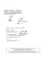
Figure 19.3.2: Worm and worm-gear operating
pitch cylinders.
Here, β
(o)
2
is the gear helix angle on the worm-gear operating pitch cylinder. The upper
sign corresponds to the case where γ>λ
(o)
1
, and the lower sign corresponds to γ<λ
(o)
1
.
Equation (19.3.6) provides the positive sign for p
t
. Similar derivations for the left-hand

worm and worm-gear (Fig. 19.2.3) yield
p
t
=
p
ax
cos λ
(o)
1
sin

γ + λ
(o)
1

. (19.3.7)
It is obvious that for the case of an orthogonal worm-gear drive (with γ = 90
◦
)we
obtain that p
t
= p
ax
.
Radius of Worm-Gear Operating Pitch Cylinder
We take into account that
p
t
N
2

= 2π R
o
. (19.3.8)
Equations (19.3.6), (19.3.7), and (19.3.8) yield the following:
(i) R
o
is represented for the right-hand worm and worm-gear as
R
o
=±
p
ax
N
2
cos λ
(o)
1
2π sin

γ − λ
(1)
o


provided γ − λ
(o)
1
= 0

. (19.3.9)

The upper sign corresponds to the case when γ>λ
(o)
1
, and the lower sign corre-
sponds to the case when γ<λ
(o)
1
.
(ii) For the left-hand worm and worm-gear, we have
R
o
=
p
ax
N
2
cos λ
(o)
1
2π sin

γ + λ
(o)
1

. (19.3.10)
P1: JsY
CB672-19 CB672/Litvin CB672/Litvin-v2.cls February 27, 2004 1:28
19.3 Design Parameters and Their Relations 555
Representation of m

21
in Terms of N
1
and N
2
The gear ratio m
21
was represented for the right-hand and left-hand worms and worm-
gears by Eqs. (19.2.8) and (19.2.9), respectively. Equations (19.2.8), (19.2.9), (19.3.9),
and (19.3.10) yield
m
21
=
N
1
N
2
. (19.3.11)
Shortest Distance E
The shortest distance E between the axes of the worm and the worm-gear is
E = r
o
+ R
o
(19.3.12)
where
r
o
=
N

1
p
ax
2π tan λ
(o)
1
, (19.3.13)
and R
o
is represented by Eq. (19.3.9) or Eq. (19.3.10). For the case when γ = 90
◦
and
the operating pitch cylinders coincide with the ordinary pitch cylinders, we obtain
E =
p
ax
2π

N
1
tan λ
(o)
1
+ N
2

. (19.3.14)
Relations Between Profile Angles in Axial, Normal,
and Transverse Sections
Consider the transverse, normal, and axial sections of the worm surface. The transverse

section is obtained by cutting of the surface by plane z = 0 [Fig. 19.3.3(a)]. The axial sec-
tion is obtained by cutting of the surface by plane y = 0 [Fig. 19.3.3(d)]. Figure 19.3.3(b)
shows the unit tangent a to the helix on the pitch cylinder at point P of the helix. The
normal section [Fig. 19.3.3(c)] is obtained by cutting of the surface by plane  that
passes through the x axis and is perpendicular to vector a [Fig. 19.3.3(b)]. The normal
section is shown in Fig. 19.3.3(c), and the unit tangent to the profile at point P is b.
The unit normal n to the worm surface at P is represented as
n = a ×b (19.3.15)
where
a = [0 cos λ
p
sin λ
p
]
T
b = [
cos α
n
sin α
n
sin λ
p
−sin α
n
cos λ
p
]
T
,
(19.3.16)

and λ
p
is the lead angle of the helix at the pitch cylinder. Equations (19.3.15) and
(19.3.16) yield
n = [
−sin α
n
cos α
n
sin λ
p
−cos α
n
cos λ
p
]
T
. (19.3.17)
Projections of the unit normal are shown in Fig. 19.3.3. The orientations of the
tangents to the profiles in the transverse, normal, and axial sections are represented by
P1: JsY
CB672-19 CB672/Litvin CB672/Litvin-v2.cls February 27, 2004 1:28
556 Worm-Gear Drives with Cylindrical Worms
Figure 19.3.3: Sections of worm sur-
face: (a) tooth cross section; (b) worm
pitch cylinder in 3D-space; (c) section
of pitch cylinder by plane ; (d) axial
section of worm tooth.
angles α
t

, α
n
, and α
ax
, respectively. It is evident from Fig. 19.3.3 that
tan α
t
=−
n
x
n
y
=
tan α
n
sin λ
p
, tan α
ax
=
n
x
n
z
=
tan α
n
cos λ
p
.

Thus,
tan α
n
= tan α
t
sin λ
p
= tan α
ax
cos λ
p
. (19.3.18)
Equation (19.3.18) relates the profile angles in normal, transverse, and axial sections.
Let us now consider a particular case, an involute worm. We may express the radius
r
b
of the base cylinder of an involute worm in terms of the screw parameter p, the lead
angle on the pitch cylinder λ
p
, and the axial profile angle α
ax
. The derivations are based
P1: JsY
CB672-19 CB672/Litvin CB672/Litvin-v2.cls February 27, 2004 1:28
19.4 Generation and Geometry of ZA Worms 557
on the following considerations:
cos α
t
=
r

b
r
p
=
tan λ
p
tan λ
b
. (19.3.19)
Equation (19.3.18) yields
tan α
t
=
tan α
ax
tan λ
p
. (19.3.20)
The radius of the base cylinder is represented as
r
b
=
p
tan λ
b
=
p
tan λ
p
cos α

t
=
p
tan λ
p
(1 + tan
2
α
t
)
1/2
. (19.3.21)
Equations (19.3.20) and (19.3.21) yield the following final expression for r
b
:
r
b
=
p
(tan
2
α
ax
+ tan
2
λ
p
)
1/2
. (19.3.22)

19.4 GENERATION AND GEOMETRY OF ZA WORMS
The worm is generated by a straight-lined blade (Fig. 19.4.1). The cutting edges of the
blade are installed in the axial section of the worm.
Henceforth we consider two generating lines, I and II, that generate the surface sides I
and II of the worm space, respectively (Fig. 19.4.2). The generating lines are represented
in coordinate system S
b
that is rigidly connected to the blade. The respective surfaces of
both sides of the worm thread are generated while coordinate system S
b
performs the
screw motion about the worm axis (Fig. 19.4.3). The generated surface is represented
in coordinate system S
1
by the matrix equation
r
1
(u,θ) = M
1b
(θ) r
b
(u). (19.4.1)
Here, the coordinate system S
1
is rigidly connected to the worm; θ is the angle of
rotation in the screw motion; parameter u determines the location of a current point
on the generating line and is measured from the point of intersection of the generating
line with the z
b
axis. Thus u =|BB


| for the current point B

of the left generating line
II. Similarly, u =|
AA

| for the current point A

of the right generating line I.
Figure 19.4.1: Installation of blade for generation of an Archimedes worm.
P1: JsY
CB672-19 CB672/Litvin CB672/Litvin-v2.cls February 27, 2004 1:28
558 Worm-Gear Drives with Cylindrical Worms
Figure 19.4.2: Geometry of straight-lined blade.
The unit surface normal is represented in coordinate system S
1
by the equations
n
1
(u,θ) =±k N
1
=±k

∂r
1
∂u
×
∂r
1

∂θ

(19.4.2)
where k = 1/|N
1
|. The upper or lower sign must be chosen with the condition that the
surface unit normal will be directed toward the worm thread.
Matrix M
1b
is represented by the equation (Fig. 19.4.3)
M
1b
=







cos θ −sin θ 00
sin θ cos θ 00
001±pθ
0001








. (19.4.3)
Figure 19.4.3: Coordinate transformation in the
case of screw motion.
P1: JsY
CB672-19 CB672/Litvin CB672/Litvin-v2.cls February 27, 2004 1:28
19.4 Generation and Geometry of ZA Worms 559
Here, p is the screw parameter that is considered as an arithmetic value (p > 0). The
upper and lower signs for pθ correspond to the cases when a right-hand worm and
a left-hand worm are generated, respectively. Figure 19.4.3 shows the generation of a
right-hand worm. The surface sides I and II for right-hand and left-hand worms are
generated by generating line I and generating line II, respectively.
Using Eqs. (19.4.1) and (19.4.2) we may represent the surface equations and the
surface unit normals for both sides of the worm thread in S
1
as follows:
(i) Surface side I, right-hand worm:
x
1
= u cos α cos θ
y
1
= u cos α sin θ
z
1
=−u sin α +

r
p
tan α −

s
p
2

+ pθ.
(19.4.4)
The surface unit normal is
n
1
=−k[(p sin θ + u sin α cos θ) i
1
− ( p cos θ −u sin α sin θ) j
1
+ u cos α k
1
]
(provided cos α = 0) (19.4.5)
where k = 1/( p
2
+ u
2
)
0.5
. We recall that parameter u is measured along the gen-
erating line I from point A of intersection of this line with axis z
b
(Fig. 19.4.2).
Design parameter s
p
is equal to the axial width w

ax
of the worm space in the axial
section. For standard worm gear drives we have
w
ax
=
π
2P
ax
(19.4.6)
where P
ax
is the axial diametral pitch.
(ii) Surface side II, right-hand worm:
x
1
= u cos α cos θ
y
1
= u cos α sin θ
z
1
= u sin α −

r
p
tan α −
s
p
2


+ pθ.
(19.4.7)
The surface unit normal is
n
1
= k[(p sin θ −u sin α cos θ) i
1
− ( p cos θ +u sin α sin θ) j
1
+ u cos α k
1
]
(provided cos α = 0) (19.4.8)
where k = 1/(p
2
+ u
2
)
0.5
.
(iii) Surface side I, left-hand worm:
x
1
= u cos α cos θ
y
1
= u cos α sin θ
z
1

=−u sin α +

r
p
tan α −
s
p
2

− pθ.
(19.4.9)
The surface unit normal is
n
1
=−k[(−p sin θ + u sin α cos θ) i
1
+ ( p cos θ +u sin α sin θ) j
1
+ u cos α k
1
]
(provided cos α = 0) (19.4.10)
where k = 1/(p
2
+ u
2
)
0.5
.
P1: JsY

CB672-19 CB672/Litvin CB672/Litvin-v2.cls February 27, 2004 1:28
560 Worm-Gear Drives with Cylindrical Worms
(iv) Surface side II, left-hand worm:
x
1
= u cos α cos θ
y
1
= u cos α sin θ
z
1
= u sin α −

r
p
tan α −
s
p
2

− pθ.
(19.4.11)
The surface unit normal is
n
1
= k[−(p sin θ +u sin α cos θ) i
1
+ ( p cos θ −u sin α sin θ) j
1
+ u cos α k

1
]
(provided cos α = 0) (19.4.12)
where k = 1/(p
2
+ u
2
)
0.5
.
Problem 19.4.1
The worm surface 
1
is represented by Eqs. (19.4.7). Consider the axial section of 
1
as the intersection of 
1
by plane y
1
= 0. Equations (19.4.7) with y
1
= 0 provide two
solutions:
(i) Derive the equations of two axial sections as x
1
= x
1
(u), and z
1
= z

1
(u).
(ii) Determine coordinates x
1
and z
1
for the point of intersection of the respective axial
section with the pitch cylinder of radius r
p
.
Solution
(i) Solution 1
x
1
= u cos α, y
1
= 0, z
1
= u sin α −

r
p
tan α −
s
p
2

.
Solution 2
x

1
=−u cos α, y
1
= 0, z
1
= u sin α −

r
p
tan α −
s
p
2

+ pπ.
(ii) Solution 1
θ = 0, x
1
= r
p
, z
1
=
s
p
2
.
Solution 2
θ = π, x
1

=−r
p
, z
1
=
s
p
2
+ pπ.
Problem 19.4.2
The worm surface 
1
is represented by Eqs. (19.4.7). Consider the cross section of 
1
by plane z
1
= 0. Investigate the equation r
1
= r
1
(θ), where r
1
= (x
2
1
+ y
2
1
)
0.5

, and verify
that it represents the Archimedes spiral.
Solution
(i) Equation z
1
= 0 yields
u =
r
p
tan α −
s
p
2
− pθ
sin α
=
a − pθ
sin α
.
P1: JsY
CB672-19 CB672/Litvin CB672/Litvin-v2.cls February 27, 2004 1:28
19.5 Generation and Geometry of ZN Worms 561
Figure 19.4.4: Cross section of an Archimedes
worm.
(ii) The cross section is represented by equations
x
1
= (a − pθ) cot α cos θ, y
1
= (a − pθ) cot α sin θ.

(iii) Equation
r
1
=

x
2
1
+ y
2
1

0.5
yields
r
1
= (a − pθ) cot α.
The magnitude of the initial position vector for θ = 0isr
1
= a cot α. The increment
and decrement of the magnitude of the position vector is proportional to θ, and this is
the proof that the cross section is an Archimedes spiral. Figure 19.4.4 shows the cross
section of the ZA worm with three threads.
19.5 GENERATION AND GEOMETRY OF ZN WORMS
Generation
ZA worms are used if the lead angle of the worm is small enough (λ
p
≤ 10
◦
). In the

case of generation of worms with large lead angles, the blade is installed as shown
in Figs. 19.5.1(a) or (b) to provide better conditions of cutting. The first version of
installation [Fig. 19.5.1(a)] provides straight-lined shapes in the normal section of the
thread. Straight-lined shapes are provided in the normal section of the space with the
second version of installation [Fig. 19.5.1(b)]. The surfaces of the worm will be generated
by the blade performing a screw motion with respect to the worm.
To describe the installation of the blade with respect to the worm, we use coordinate
systems S
a
and S
b
that are rigidly connected to the blade and the worm. We start the
discussion with the generation of the worm space (Fig. 19.5.2). Axis z
b
coincides with
P1: JsY
CB672-19 CB672/Litvin CB672/Litvin-v2.cls February 27, 2004 1:28
562 Worm-Gear Drives with Cylindrical Worms
Figure 19.5.1: Blade installation for genera-
tion of ZN worm: (a) for thread generation;
(b) for space generation.
Figure 19.5.2: Coordinate systems applied for blade in-
stallation.
P1: JsY
CB672-19 CB672/Litvin CB672/Litvin-v2.cls February 27, 2004 1:28
19.5 Generation and Geometry of ZN Worms 563
Figure 19.5.3: Representation of generating lines in
coordinate system S
a
.

the worm axis; axes z
a
and z
b
form angle λ
p
that is the lead angle on the worm pitch
cylinder; the origins O
a
and O
b
lie on the worm axis.
The straight-lined shapes of the blades are shown in Fig. 19.5.3. The extended straight
lines are in tangency with the cylinder of the to-be-determined radius ρ. The intersection
of plane y
a
= 0 of coordinate system S
a
with the cylinder represents an ellipse with axes
2ρ and 2ρ/sin λ
p
. The coordinate transformation from S
a
to S
b
is represented by the
matrix M
ba
:
M

ba
=







10 00
0 cos λ
p
∓sin λ
p
0
0 ±sin λ
p
cos λ
p
0
00 01







. (19.5.1)
The upper and lower signs correspond to the generation of a right-hand worm and

left-hand worm, respectively.
P1: JsY
CB672-19 CB672/Litvin CB672/Litvin-v2.cls February 27, 2004 1:28
564 Worm-Gear Drives with Cylindrical Worms
Figure 19.5.4: Interpretation of ellipse equations.
Representation of Generating Lines in Coordinate Systems S
a
Henceforth we consider the generating lines I and II (Fig. 19.5.3). Each generating line
is tangent to the ellipse whose equations are represented in S
a
in parametric form as
R
a
=

ρ sin µ 0
ρ
sin λ
p
cos µ

T
. (19.5.2)
Figure 19.5.4 illustrates the determination of coordinates of current point C of the
ellipse; µ is the variable parameter.
The unit tangent τ
a
to the ellipse is represented by the equation
τ
a

=
T
a
|T
a
|
=
ρ
|T
a
|

cos µ 0 −
sin µ
sin λ
p

T

T
a
=
dR
a
dµ

. (19.5.3)
The direction of τ
a
that is shown in Fig. 19.5.3 coincides with the direction of increment

of parameter µ (Fig. 19.5.4).
The unit vectors b
(i )
a
(i = I, II) of the generating lines I and II are represented in S
a
as follows:
b
(I )
a
= [
cos α 0 −sin α
]
T
(19.5.4)
b
(II )
a
= [
cos α 0 sin α
]
T
. (19.5.5)
It is evident that at the point of tangency of the generating line with the ellipse (point
M and respectively M

), we have b
(I )
a
= τ

(I )
a
and b
(II )
a
=−τ
(II )
a
. Equations (19.5.3),
(19.5.4), and (19.5.5) yield (see additional explanations in Notes 1 and 2, which
P1: JsY
CB672-19 CB672/Litvin CB672/Litvin-v2.cls February 27, 2004 1:28
19.5 Generation and Geometry of ZN Worms 565
follow this section)
ρ
|T
a
|
= cos δ, cos µ
(I )
=
cos α
cos δ
sin µ
(I )
=
sin α sin λ
p
cos δ
= tan δ tan λ

p
cos µ
(II )
=−
cos α
cos δ
, sin µ
(II )
=
sin α sin λ
p
cos δ
= tan δ tan λ
p
.
(19.5.6)
Here,
cos δ = (cos
2
α + sin
2
α sin
2
λ
p
)
0.5
, sin δ = sin α cos λ
p
. (19.5.7)

The designations “I” and “II” indicate the generating lines I and II.
The generating lines are represented in S
a
by the equations
x
a
= ρ sin µ ± u cos δ cos µ
y
a
= 0
z
a
=
ρ cos µ
sin λ
p
∓ u
cos δ sin µ
sin λ
p
.
(19.5.8)
The upper and lower signs in Eqs. (19.5.8) correspond to the generating lines I and II,
respectively. The designations “I” and “II” have been dropped but the magnitudes of
µ are different for generating lines I and II [see Eqs. (19.5.6)]. Parameter u determines
the location of current point A (or A

) on the generating line; u =|MA| and u =|M

A


|
as shown in Fig. 19.5.3.
Note 1: Determination of Expressions for cos δ and sin δ
Using the equality b
(I )
a
= τ
(I )
a
, and Eqs. (19.5.3) and (19.5.4), we obtain
ρ
|T
a
|
cos µ
(I )
= cos α,
ρ
|T
a
|
sin µ
(I )
sin λ
p
= sin α. (19.5.9)
Equations (19.5.9) yield
cos µ
(I )

=

ρ
|T
a
|

−1
cos α, sin µ
(I )
=

ρ
|T
a
|

−1
sin α sin λ
p
. (19.5.10)
Using Eqs. (19.5.10), we obtain that
ρ
|T
a
|
= (cos
2
α + sin
2

α sin
2
λ
p
)
0.5
. (19.5.11)
Using for the purpose of simplification the designation
ρ
|T
a
|
= cos δ, (19.5.12)
we obtain the following expressions for cos δ and sin δ:
cos δ = (cos
2
α + sin
2
α sin
2
λ
p
)
0.5
, sin δ = (1 − cos
2
δ)
0.5
= sin α cos λ
p

.
Equations (19.5.7) are confirmed.
P1: JsY
CB672-19 CB672/Litvin CB672/Litvin-v2.cls February 27, 2004 1:28
566 Worm-Gear Drives with Cylindrical Worms
Note 2: Derivation of Expressions for cos µ and sin µ
Equations (19.5.9) yield
cos µ
(I )
=
cos α
cos δ
, sin µ
(I )
=
sin α sin λ
p
cos δ
(19.5.13)
because |ρ/T
a
|=cos δ.
Taking into account that sin δ = sin α cos λ
p
[see Eqs. (19.5.7)], we obtain
cos µ
(I )
=
cos α
cos δ

, sin µ
(I )
= tan δ tan λ
p
. (19.5.14)
Similarly, we can derive the expressions for cos µ
(II )
and sin µ
(II )
. The expressions
for cos µ
(i )
, sin µ
(i )
(i = I, II) have been represented in Eqs. (19.5.6).
Determination of ρ
Equations (19.5.8) represent generating lines that are tangents to the ellipse shown in
Fig. 19.5.3. The points of tangency are M and M

, respectively. Equations (19.5.8) for
point N of the generating lines (Fig. 19.5.3) are represented as
ρ sin µ ± u
∗
cos δ cos µ = d,
ρ cos µ
sin λ
p
∓
u
∗

cos δ sin µ
sin λ
p
= 0 (19.5.15)
where u
∗
=|MN|=|M

N|, d = O
a
N = r
p
− (s
p
/2) cot α.
We consider Eqs. (19.5.15) as a system of two linear equations in the unknowns u
∗
and ρ and represent them as
a
11
ρ + a
12
u
∗
= d, a
21
ρ + a
22
u
∗

= 0. (19.5.16)
The solution for the unknown ρ is
ρ =

1

(19.5.17)
where

1
=





da
12
0 a
22





=∓

d cos δ sin µ
sin λ
p


(19.5.18)
 =





a
11
a
12
a
21
a
22





=∓

cos δ
sin λ
p

. (19.5.19)
Equations (19.5.16) to (19.5.19) yield
ρ = d

sin α sin λ
p
(cos
2
α + sin
2
α sin
2
λ
p
)
0.5
(19.5.20)
where
d = r
p
−
s
p
2
cot α.
P1: JsY
CB672-19 CB672/Litvin CB672/Litvin-v2.cls February 27, 2004 1:28
19.5 Generation and Geometry of ZN Worms 567
Figure 19.5.5: Worm thread generation [Fig.
19.5.1(a)]: representation of generating lines in
S
a
.
For the case where the blades are installed as shown in Fig. 19.5.1(a), we obtain that

(Fig. 19.5.5)
d = r
p
+
w
p
2
cot α. (19.5.21)
Here, w
p
is the distance between the blades measured as shown in Fig. 19.5.5.
Equations of Surfaces of Worm Thread
The surface of the worm thread is generated by the edge of the blade (the generating
line) that performs a screw motion about the worm axis. The vector equation of the
surface is represented in S
1
by the following matrix equation:
r
1
(θ,u) = M
1b
(θ)M
ba
r
a
(u). (19.5.22)
Here, r
a
(u) is the vector equation of the generating line that is represented in coordinate
system S

a
; matrix M
ba
is represented by (19.5.1); matrix M
1b
is represented by (19.4.3).
The surface unit normal is represented as follows:
n
1
(u,θ) =±
N
1
|N
1
|
, N
1
=
∂r
1
∂u
×
∂r
1
∂θ
. (19.5.23)
Choosing the proper sign in Eqs. (19.5.23), we may obtain that the surface normal will
be directed toward the worm thread.
Surfaces and surface unit normals of ZN worms are represented as follows:
(i) Surface side I, right-hand worm:

x
1
= ρ sin(θ +µ) +u cos δ cos(θ + µ)
y
1
=−ρ cos(θ + µ) + u cos δ sin(θ + µ)
z
1
= ρ
cos α cot λ
p
cos δ
− u sin δ + pθ.
(19.5.24)
P1: JsY
CB672-19 CB672/Litvin CB672/Litvin-v2.cls February 27, 2004 1:28
568 Worm-Gear Drives with Cylindrical Worms
Here,
cos µ =
cos α
cos δ
, sin µ =
sin α sin λ
p
cos δ
,
cos δ = (cos
2
α + sin
2

α sin
2
λ
p
)
1/2
, sin δ = sin α cos λ
p
.
(19.5.25)
Surface unit normal components:
n
x1
=−
1
k
[(p + ρ tan δ) sin(θ + µ) +u sin δ cos(θ + µ)]
n
y1
=−
1
k
[−(p + ρ tan δ) cos(θ + µ) +u sin δ sin(θ + µ)]
n
z1
=−
u cos δ
k
.
(19.5.26)

Here,
k = [(p +ρ tan δ)
2
+ u
2
]
0.5
.
(ii) Surface side II, right-hand worm:
x
1
= ρ sin(θ +µ) −u cos δ cos(θ + µ)
y
1
=−ρ cos(θ + µ) − u cos δ sin(θ + µ)
z
1
=−ρ
cos α cot λ
p
cos δ
+ u sin δ + pθ.
(19.5.27)
Here, cos µ =−cos α/cos δ, sin µ = sin α sin λ
p
/cos δ; the expressions for cos δ
and sin δ are the same as those in Eqs. (19.5.25).
Surface unit normal components:
n
x1

=
1
k
[−(p + ρ tan δ) sin(θ + µ) +u sin δ cos(θ + µ)]
n
y1
=
1
k
[(p + ρ tan δ) cos(θ + µ) +u sin δ sin(θ + µ)]
n
z1
=
u cos δ
k
.
(19.5.28)
(iii) Surface side I, left-hand worm:
x
1
=−ρ sin(θ − µ) + u cos δ cos(θ − µ)
y
1
= ρ cos(θ −µ) +u cos δ sin(θ − µ)
z
1
= ρ
cos α cot λ
p
cos δ

− u sin δ − pθ.
(19.5.29)
Here,
cos µ =
cos α
cos δ
, sin µ =
sin α sin λ
p
cos δ
= tan δ tan λ
p
. (19.5.30)
P1: JsY
CB672-19 CB672/Litvin CB672/Litvin-v2.cls February 27, 2004 1:28
19.5 Generation and Geometry of ZN Worms 569
Surface unit normal components:
n
x1
=
1
k
[(p + ρ tan δ) sin(θ − µ) −u sin δ cos(θ − µ)]
n
y1
=
1
k
[−(p + ρ tan δ) cos(θ − µ) −u sin δ sin(θ − µ)]
n

z1
=−
u cos δ
k
.
(19.5.31)
(iv) Surface side II, left-hand worm:
x
1
=−ρ sin(θ − µ) − u cos δ cos(θ − µ)
y
1
= ρ cos(θ −µ) −u cos δ sin(θ − µ)
z
1
=−ρ
cos α cot λ
p
cos δ
+ u sin δ − pθ.
(19.5.32)
Here,
cos µ =−
cos α
cos δ
, sin µ =
sin α sin λ
p
cos δ
= tan δ tan λ

p
. (19.5.33)
Surface unit normal components:
n
x1
=
1
k
[(p + ρ tan δ) sin(θ − µ) +u sin δ cos(θ − µ)]
n
y1
=
1
k
[−(p + ρ tan δ) cos(θ − µ) +u sin δ sin(θ − µ)]
n
z1
=
u cos δ
k
.
(19.5.34)
Kinematic Interpretation of Surface Generation
The visualization of generation of the worm surface is based on the following consid-
erations:
(i) The generating line L
( j )
( j = I, II) may be represented in plane 
( j )
that is tangent

to the cylinder of radius ρ (superscripts I and II indicate the generating lines I and
II, respectively).
(ii) L
( j )
and the worm axis represent two crossed straight lines. Thus, L
( j )
may be
represented in a coordinate system S
τ
( j )
whose unit vectors we designate as e
( j )
1
,
e
( j )
2
, and e
( j )
3
. The unit vector e
( j )
3
is directed along the worm axis and e
( j )
3
= k
b
.
Unit vector e

( j )
1
is directed along the shortest distance between the unit vectors of
the generating line and the worm axis. Unit vector e
( j )
2
is determined as the cross
product of e
( j )
1
and e
( j )
3
(see below).
(iii) Coordinate systems S
( j )
τ
( j = I, II) and S
b
(Figs. 19.5.6 and 19.5.7) are rigidly
connected to each other and perform a screw motion with the screw parameter p
about the worm axis. Point M
( j )
of the intersection of L
( j )
with e
( j )
1
generates in
screw motion a helix on the cylinder of radius ρ. The unit tangent to the helix at

point M
( j )
and the unit vector b
( j )
of L
( j )
do not coincide in the case of ZN worms
and form a certain angle.
P1: JsY
CB672-19 CB672/Litvin CB672/Litvin-v2.cls February 27, 2004 1:28
570 Worm-Gear Drives with Cylindrical Worms
Figure 19.5.6: Representation of generating line
I in S
τ
.
(iv) We may consider now two rigidly connected straight lines with unit vectors b
( j )
and τ that lie in tangent plane 
( j )
and have a common point M
( j )
as the point of
their intersection. Both of these straight lines perform the same screw motion, and
straight line L
( j )
generates the worm surface that is a convolute surface. Line L
( j )
would generate a screw involute surface if L
( j )
were to coincide with τ

( j )
.
For further derivations, we consider the following equation:
O
b
N = O
b
O
( j )
τ
+ O
( j )
τ
M
( j )
+ M
( j )
N. (19.5.35)
Here, N is the point of intersection of both generating lines (Fig. 19.5.3), and
O
b
N = d i
b
. (19.5.36)
Figure 19.5.7: Representation of generating
line II in S
τ
.
P1: JsY
CB672-19 CB672/Litvin CB672/Litvin-v2.cls February 27, 2004 1:28

19.5 Generation and Geometry of ZN Worms 571
Vectors O
b
O
( j )
τ
, O
( j )
τ
M
( j )
, and M
( j )
N may be represented in S
b
as
O
b
O
( j )
τ
= λ
( j )
k
b
( j = I, II) (19.5.37)
O
( j )
τ
M

( j )
= ρ e
( j )
1b
(19.5.38)
where
e
( j )
1b
=±
b
( j )
b
× k
b


b
( j )
b
× k
b


(19.5.39)
M
( j )
N = m b
( j )
b

(19.5.40)
e
( j )
2b
= e
( j )
3b
× e
( j )
1b
. (19.5.41)
The subscript “b” in e
( j )
1b
and e
( j )
2b
indicates that these vectors are represented in S
b
.
The determination of the proper sign in Eq. (19.5.39) is based on the following
considerations:
(i) Equations (19.5.35) to (19.5.39) yield
d

i
b
· e
( j )
1b


= ρ. (19.5.42)
(ii) Taking into account that d and ρ are positive, we get
i
b
· e
( j )
1b
> 0. (19.5.43)
(iii) Equations (19.5.42) and (19.5.43) yield that the upper (lower) sign in Eq. (19.5.39)
corresponds to the case where j = I ( j = II).
Using expressions (19.5.39) and (19.5.40), we can determine the direction cosines
for vectors e
( j )
1b
and e
( j )
2b
( j = I, II) in coordinate system S
b
. We can determine as well
the location of origin O
( j )
τ
( j = I, II)inS
b
using vector equation (19.5.35). Then we
obtain the following matrices for coordinate transformation,
M
(I )

τ b
=












tan λ
p
tan δ −
cos α
cos δ
00
cos α
cos δ
tan λ
p
tan δ 00
001−
d cos α tan δ
cos δ
0001













(19.5.44)
M
(II )
τ b
=













sin α sin λ

p
cos δ
cos α
cos δ
00
−
cos α
cos δ
sin α sin λ
p
cos δ
00
001
d cos α tan δ
cos δ
0001













. (19.5.45)

P1: JsY
CB672-19 CB672/Litvin CB672/Litvin-v2.cls February 27, 2004 1:28
572 Worm-Gear Drives with Cylindrical Worms
The generating lines are represented in S
( j )
τ
by the following equations (Figs. 19.5.6
and 19.5.7):
b
(I )
τ
= [
0 cos δ −sin δ
]
T
(19.5.46)
b
(II )
τ
= [
0 −cos δ sin δ
]
T
. (19.5.47)
The tangent to the helix at point M
( j )
is represented in S
( j )
τ
by

τ
( j )
τ
= [
0 cos λ
ρ
sin λ
ρ
]
T
(19.5.48)
where
λ
ρ
= arctan

p
ρ

. (19.5.49)
Using similar derivations for a right-hand worm, we obtain the equations of gener-
ating lines for the left-hand worm. The generating lines are represented in coordinate
systems S
( j )
τ
( j = I, II) that enable us to determine the orientation of the generating
line in plane 
( j )
that is tangent to the cylinder of radius ρ (Figs. 19.5.6 and 19.5.7).
The unit vectors of the right and left generating lines are represented in S

(I )
τ
and S
(II )
τ
as follows:
b
(I )
τ
= [
0 −cos δ −sin δ
]
T
(19.5.50)
b
(II )
τ
= [
0 cos δ sin δ
]
T
. (19.5.51)
The cross section of the worm surface is an extended involute (Fig. 19.5.8) that is
traced out by point B
o
of the segment B
o
M; this segment is rigidly connected to the
Figure 19.5.8: Extended involute as the
profile of ZN worm cross section.

P1: JsY
CB672-19 CB672/Litvin CB672/Litvin-v2.cls February 27, 2004 1:28
19.5 Generation and Geometry of ZN Worms 573
Figure 19.5.9: Cross section of ZN worm.
straight line that rolls over the circle of radius p/ tan δ
ρ
. The cross section of a ZN worm
with three threads is represented in Fig. 19.5.9.
Particular Cases
The surface of Archimedes worm (ZA) is a particular case of the screw convolute surface
(ZN). Equations of surface ZA can be derived from the equations of surface ZN taking
ρ = 0 and δ = α, µ = 0 and µ = π for the surface sides I and II, respectively. The screw
involute surface can be derived from the equations of convolute screw surface (ZN) by
considering that the generating line is the tangent to the helix on the cylinder of radius
ρ (see below).
Problem 19.5.1
Consider that the worm surface represented by Eqs. (19.5.24) is cut by the plane y
1
= 0.
Axis x
1
is the axis of symmetry of the space in axial section. The point of intersection
of the axial profile with the pitch cylinder is determined with the coordinates
x
1
= r
p
, z
1
=−

w
ax
2
=−
p
ax
4
=−
π
4P
ax
.
Here, w
ax
is the nominal value of the space width in axial section that is measured along
the generatrix of the pitch cylinder; p
ax
is the distance between two neighboring threads
along the generatrix of the pitch cylinder; P
ax
= π/p
ax
is the worm axial diametral pitch.
Derive the system of equations to be applied to determine s
p
(Fig. 19.5.3) considering
r
p
, p, w
ax

, and α as given.
Solution
Angle θ can be obtained from the following equation:
r
p

sin θ
tan λ
p
+ tan λ
p
θ

+
w
ax
2
= 0. (19.5.52)
P1: JsY
CB672-19 CB672/Litvin CB672/Litvin-v2.cls February 27, 2004 1:28
574 Worm-Gear Drives with Cylindrical Worms
Then, s
p
can be expressed as
s
p
= 2r
p

(1 − cos θ) tan α −

sin θ
sin λ
p

. (19.5.53)
While solving the nonlinear equation, we take for the first guess sin θ ≈ θ.
Directions
(1) Equation (19.5.52) can be derived considering the following system of equations:
x
1
= ρ sin(θ +µ) +u cos δ cos(θ + µ) = r
p
(19.5.54)
y
1
=−ρ cos(θ + µ) + u cos δ sin(θ + µ) = 0 (19.5.55)
z
1
= ρ
cos α cot λ
p
cos δ
− u sin δ + pθ =−
w
ax
2
. (19.5.56)
Equation (19.5.55) yields
u cos δ =
ρ

tan(θ + µ)
. (19.5.57)
Equations (19.5.54) and (19.5.55) considered simultaneously yield
ρ = r
p
sin(θ + µ). (19.5.58)
We may consider Eqs. (19.5.54), (19.5.55), and (19.5.56) as a system of three
linear equations in the unknowns u and ρ. If such a system indeed exists, the rank
of the augmented matrix must be equal to 2. This requirement yields an equation
that coincides with Eq. (19.5.52) represented above.
(2) The derivation of Eq. (19.5.53) is based on the following considerations:
(a) According to Eq. (19.5.20), we have
ρ =

r
p
−
s
p
2
cot α

sin α sin λ
p
(cos
2
α + sin
2
α sin
2

λ
p
)
0.5
.
(b) We transform this equation using the substitutions [see Eqs. (19.5.58) and
(19.5.25)]
ρ = r
p
sin(θ + µ), cos µ cos δ = cos α, sin µ cos δ = sin α sin λ
p
cos δ = (cos
2
α + sin
2
α sin
2
λ
p
)
0.5
.
After transformations, we obtain Eq. (19.5.53) represented above.
19.6 GENERATION AND GEOMETRY OF ZI (INVOLUTE) WORMS
Surface Equations
The worm surface is generated by a straight line that performs a screw motion and is
tangent to the helix M
o
M on the base cylinder (Fig. 19.6.1). The position vector O
1

N
of a current point of the surface side I for a right-hand worm is represented as
O
1
N = O
1
K + KM+ MN. (19.6.1)
P1: JsY
CB672-19 CB672/Litvin CB672/Litvin-v2.cls February 27, 2004 1:28
19.6 Generation and Geometry of ZI (Involute) Worms 575
Figure 19.6.1: Generation of screw involute
surface for the surface side I of a right-hand
worm.
Here,
O
1
K = r
b
(cos θ i
1
+ sin θ j
1
), KM = pθ k
1
,
MN = u cos λ
b
(sin θ i
1
− cos θ j

1
) − u sin λ
b
k
1
(19.6.2)
where r
b
is the radius of the base cylinder, λ
b
is the helix lead angle, p = r
b
tan λ
b
is the
screw parameter, and variables u and θ are the surface parameters.
Equations (19.6.1) and (19.6.2) yield
x
1
= r
b
cos θ + u cos λ
b
sin θ
y
1
= r
b
sin θ − u cos λ
b

cos θ
z
1
=−u sin λ
b
+ pθ.
(19.6.3)
The surface unit normal directed toward the worm thread is represented by
n
1
=
N
1
|N
1
|
, N
1
=
∂r
1
∂θ
×
∂r
1
∂u
. (19.6.4)
Then we derive that
n
1

= [
−sin λ
b
sin θ sin λ
b
cos θ −cos λ
b
]
T
(19.6.5)
(provided u cos λ
b
= 0).
The orientation of surface unit normal n
1
does not depend on u. This means that the
unit normals along the generating line have the same orientation, and the worm surface
is a ruled developed one. (We recall that the surfaces of ZA worms and ZN worms are
ruled but undeveloped surfaces.)
P1: JsY
CB672-19 CB672/Litvin CB672/Litvin-v2.cls February 27, 2004 1:28
576 Worm-Gear Drives with Cylindrical Worms
Figure 19.6.2: Derivation of screw involute sur-
face for the surface side II of a right-hand worm.
It is easy to verify that N
1
= 0 when u = 0. Thus, the surface point is singular at the
point of tangency of the generating line with the helix. At such a point, vectors ∂r
1
/∂u

and ∂r
1
/∂θ are collinear.
The cross section of the worm surface by z
1
= c is an involute curve with the radius
of base circle r
b
.
The derivation of surface side II of the right-hand worm is based on drawings repre-
sented in Fig. 19.6.2. Using considerations similar to those discussed above, we obtain
the following equations for the surface and its unit normal:
x
1
= r
b
cos θ + u cos λ
b
sin θ
y
1
=−r
b
sin θ + u cos λ
b
cos θ
z
1
= u sin λ
b

− pθ
(19.6.6)
n
1
=

−sin λ
b
sin θ −sin λ
b
cos θ cos λ
b

T
(19.6.7)
(provided u cos λ
b
= 0).
Our next goal is to represent the surface equations for both sides with the x
1
axis as
the axis of symmetry for the cross section z
1
= 0. Figure 19.6.3 yields that
µ =
w
t
2r
p
− inv α

t
. (19.6.8)
Here, w
t
is the cross section space width on the pitch cylinder and α
t
is the profile angle
in transverse section (formed between the position vector O
1
P and the tangent to the
profile at point P). It is known from the involute trigonometry that
inv α
t
= tan α
t
− α
t
,α
t
= arccos

r
b
r
p

. (19.6.9)
P1: JsY
CB672-19 CB672/Litvin CB672/Litvin-v2.cls February 27, 2004 1:28
19.6 Generation and Geometry of ZI (Involute) Worms 577

Figure 19.6.3: Involute worm cross sections: (a) with profile I ; (b) with profile II.
We recall that the transverse and axial shape angles, α
t
and α
ax
, are related by
Eq. (19.3.20), and the radius of the base cylinder is represented by Eq. (19.3.21). The
final expressions for both sides of the worm surface, for right-hand and left-hand worms,
are as follows:
(i) Surface side I, right-hand worm:
x
1
= r
b
cos(θ + µ) + u cos λ
b
sin(θ + µ)
y
1
= r
b
sin(θ + µ) − u cos λ
b
cos(θ + µ)
z
1
=−u sin λ
b
+ pθ
(19.6.10)

n
1
= [
−sin λ
b
sin(θ + µ) sin λ
b
cos(θ + µ) −cos λ
b
]
T
. (19.6.11)
Angles θ and µ are measured clockwise from
O
1
M
I
to the direction of the y
1
axis
for an observer located on the negative axis z
1
.