Gear Geometry and Applied Theory Episode 3 Part 4 pptx
Bạn đang xem bản rút gọn của tài liệu. Xem và tải ngay bản đầy đủ của tài liệu tại đây (479.73 KB, 30 trang )
P1: GDZ/SPH P2: GDZ
CB672-21 CB672/Litvin CB672/Litvin-v2.cls February 27, 2004 2:1
21.9 Example of Design and Optimization of a Spiral Bevel Gear Drive 673
Figure 21.9.6: (a) and (b) bearing contact for design cases 1b and 1c, respectively, and (c) function of
transmission errors for both cases of design.
P1: GDZ/SPH P2: GDZ
CB672-21 CB672/Litvin CB672/Litvin-v2.cls February 27, 2004 2:1
Figure 21.9.7: Contact and bending stresses for the pinion for design case 1c.
Figure 21.9.8: Contact and bending stresses for the gear for design case 1c.
674
P1: GDZ/SPH P2: GDZ
CB672-21 CB672/Litvin CB672/Litvin-v2.cls February 27, 2004 2:1
21.9 Example of Design and Optimization of a Spiral Bevel Gear Drive 675
Figure 21.9.9: Evolution of contact and bending stresses for the pinion for design cases 1a, 1b, and
1c.
case 1c enables us to avoid the appearance of a small area of severe contact at the top
edge of the pinion with a higher level of contact stresses as shown in Figure 21.9.9(a).
On the contrary, bending stresses for design cases 1b and 1c are higher than they are
for the existing case of design as shown in Fig. 21.9.9(b).
A substantial reduction of contact stresses could be achieved as well for the gear for
design cases 1b and 1c with respect to the existing design of the gear of the gear drive.
The same results as previously discussed for the pinion have been obtained for the gear
for design cases 1b and 1c as shown in Fig. 21.9.10.
P1: GDZ/SPH P2: GDZ
CB672-21 CB672/Litvin CB672/Litvin-v2.cls February 27, 2004 2:1
676 Spiral Bevel Gears
Figure 21.9.10: Evolution of contact and bending stresses for the gear for design cases 1a, 1b, and 1c.
21.10 COMPENSATION OF THE SHIFT OF THE BEARING CONTACT
Spiral bevel gear drives are very sensitive to the shortest distance between the axes
of the pinion and the gear, E, when the pinion–gear axes are not intersected but
crossed. However, the shift of the bearing contact due to error of alignment E can
be compensated by the axial displacement A
1
of the pinion. Figure 21.10.1 shows
an example of compensation of an error of alignment E = 0.02 mm for design
case 1c.
Figure 21.10.1(a) shows the path of contact for design case 1c when no errors of
alignment occur. Figure 21.10.1(b) shows the path of contact for an error of alignment
P1: GDZ/SPH P2: GDZ
CB672-21 CB672/Litvin CB672/Litvin-v2.cls February 27, 2004 2:1
21.10 Compensation of the Shift of the Bearing Contact 677
Figure 21.10.1: Design case 1c: (a) path of contact when no errors of alignment occur, (b) path of
contact for error of alignment E = 0.02 mm, (c) path of contact when error of alignment E =
0.02 mm is compensated by A
1
=−0.05 mm, (d) function of transmission errors for conditions of
item (c).
P1: GDZ/SPH P2: GDZ
CB672-21 CB672/Litvin CB672/Litvin-v2.cls February 27, 2004 2:1
678 Spiral Bevel Gears
E = 0.02 mm. Figure 21.10.1(c) shows the path of contact for an error of alignment
E = 0.02 mm and an axial displacement of the pinion A
1
=−0.05 mm. As shown
in Fig. 21.10.1(c), an axial displacement of the pinion may compensate the shift of the
path of contact caused by an error E of the shortest distance between axes. Figure
21.10.1(d) shows the function of transmission errors when an error of alignment E =
0.02 mm is compensated by an axial displacement of the pinion A
1
=−0.05 mm.
The function of transmission errors is still of parabolic shape.
P1: JDW
CB672-22 CB672/Litvin CB672/Litvin-v2.cls February 27, 2004 2:3
22 Hypoid Gear Drives
22.1 INTRODUCTION
Hypoid gear drives have found a broad application in the automotive industry for
transformation of rotation between crossed axes. Enhanced design and generation of
hypoid gear drives requires an approach based on the ideas discussed for spiral bevel
gears (see Chapter 21).
The contents of this chapter are limited to (i) design of pitch cones, (ii) pinion and
gear machine-tool settings, and (iii) equations of pinion–gear tooth surfaces. Design of
pitch cones for hypoid gears was the subject of research performed by Baxter [1961],
Litvin et al. [1974, 1990] and Litvin [1994]. Details of determination of machine-tool
settings for manufacture of hypoid gears are given in Litvin & Gutman [1981].
22.2 AXODES AND OPERATING PITCH CONES
Spiral bevel gears perform rotation about intersected axes, and their axodes are two
cones (Section 3.4). The line of tangency of these cones is the instantaneous axis of
rotation in relative motion. In the case of standard spiral bevel gears, the gear axodes
coincide with the pitch cones.
Hypoid gears perform rotation about crossed axes, the relative motion is a screw
motion, and instead of the instantaneous axis of rotation we have to consider the in-
stantaneous screw axis s–s (Section 3.5). The gear axodes are two hyperboloids of
revolution that are in tangency along the axis of screw motion s–s (Fig. 3.5.1). The
hypoid pinion–gear axodes (the hyperboloids of revolution) perform in relative motion
rotation about and translation along s–s.
The concept of axodes of hypoid gears has found a limited application in design and
is used merely for visualization of relative velocity. The main reason for this is that the
location of axodes is out of the zone of meshing of hypoid gears.
The design of blanks of hypoid gears is meant to determine operating pitch cones
instead of hyperboloids of revolution, the hypoid gear axodes. The operating pitch
cones (Fig. 22.2.1) must satisfy the following requirements:
(a) The axes of the pitch cones form the prescribed crossing angle γ between the axes
of rotation (usually, γ = 90
◦
).
679
P1: JDW
CB672-22 CB672/Litvin CB672/Litvin-v2.cls February 27, 2004 2:3
680 Hypoid Gear Drives
Figure 22.2.1: Operating pitch cones of
hypoid gears.
(b) The shortest distance E between the axes of the pitch cones is equal to the prescribed
value of the hypoid gear drive.
(c) The pitch cones are in tangency at the prescribed point P that is located in the zone
of meshing of the pinion–gear tooth surfaces.
(d) The relative (sliding) velocity at point P is directed along the common tangent to
the “helices” of contacting pitch cones. The term “helix” is used to denote a curve
obtained by intersection of the tooth surface by the pitch cone.
22.3 TANGENCY OF HYPOID PITCH CONES
A cone is represented in coordinate system S
i
by the equations (Fig. 22.3.1)
x
i
= u
i
sin γ
i
cos θ
i
y
i
= u
i
sin γ
i
sin θ
i
(i = 1, 2)
z
i
= u
i
cos γ
i
(22.3.1)
Figure 22.3.1: Operating pitch cone and its param-
eters.
P1: JDW
CB672-22 CB672/Litvin CB672/Litvin-v2.cls February 27, 2004 2:3
22.3 Tangency of Hypoid Pitch Cones 681
where (u
i
, θ
i
) are the surface coordinates (the Gaussian coordinates). The surface unit
normal is represented by the equations
n
i
=
N
i
|N
i
|
, N
i
=
∂r
i
∂u
i
×
∂r
i
∂θ
i
. (22.3.2)
Equations (22.3.1) and (22.3.2) yield (providing u
i
sin γ
i
= 0)
n
i
= [cos θ
i
cos γ
i
sin θ
i
cos γ
i
− sin γ
i
]
T
. (22.3.3)
To derive the equations of tangency of the pitch cones at the pitch point P , we represent
the pitch cones in the fixed coordinate system S
f
.
The location and orientation of coordinate systems S
1
and S
2
with respect to S
f
are
shown in Fig. 22.4.1. Coordinate transformation from S
1
and S
2
to S
f
allows us to
represent in coordinate system S
f
the pitch cones of the pinion and the gear and their
unit normals by the following vector functions:
r
(1)
f
(u
1
,θ
1
) =
r
1
cos θ
1
r
1
sin θ
1
r
1
cot γ
1
− d
1
(22.3.4)
n
(1)
f
(θ
1
) =
cos γ
1
cos θ
1
cos γ
1
sin θ
1
−sinγ
1
(22.3.5)
r
(2)
f
(u
2
,θ
2
) =
r
2
cos θ
2
+ E
−r
2
cot γ
2
+ d
2
r
2
sin θ
2
(22.3.6)
n
(2)
f
(θ
2
) =
−cosγ
2
cos θ
2
−sinγ
2
−cosγ
2
sin θ
2
. (22.3.7)
Here, d
i
(i = 1, 2) determines the location of the apex of the pitch cone.
The pitch cones are in tangency at the pitch point P , and the equations of tangency
are
r
(1)
f
(u
1
,θ
1
) = r
(2)
f
(u
2
,θ
2
) = r
(P)
f
(22.3.8)
n
(1)
f
(θ
1
) = n
(2)
f
(θ
2
) = n
(P)
f
(22.3.9)
where r
(P)
f
and n
(P)
f
are the position vector and the common normal to the pitch cones
at pitch point P. The mating pitch cones are located above and below the pitch plane.
Therefore, their surface unit normals have opposite directions at P and the coincidence
of the surface unit normals is provided with the negative sign in Eq. (22.3.9).
Vector equations (22.3.8) and (22.3.9) provide the six scalar equations
r
1
cos θ
1
= r
2
cos θ
2
+ E = x
(P)
f
(22.3.10)
r
1
sin θ
1
=−r
2
cos θ
2
+ d
2
= y
(P)
f
(22.3.11)
r
1
cot γ
1
− d
1
= r
2
sin θ
2
= z
(P)
f
, (22.3.12)
P1: JDW
CB672-22 CB672/Litvin CB672/Litvin-v2.cls February 27, 2004 2:3
682 Hypoid Gear Drives
where r
i
= u
i
sin γ
i
is the radius of the pitch cone at P, and
cos γ
i
cos θ
i
=−cos γ
2
cos θ
2
= n
(P)
xf
(22.3.13)
cos γ
i
sin θ
i
=−sin γ
2
= n
(P)
yf
(22.3.14)
−sinγ
1
=−cos γ
2
sin θ
2
= n
(P)
zf
. (22.3.15)
Only two equations of the equation system (22.3.13) to (22.3.15) are independent
because |n
(1)
f
|=|n
(2)
f
|=1.
Eliminating cos θ
i
and sin θ
i
, we obtain after some transformation the following equa-
tions:
r
1
r
2
=
(E/r
2
) cosγ
1
cos
2
γ
1
− sin
2
γ
2
−
cos γ
1
cos γ
2
(22.3.16)
d
1
=−
r
2
cos γ
2
sin γ
1
+
E cos γ
1
cot γ
1
cos
2
γ
1
− sin
2
γ
2
(22.3.17)
d
2
=
r
2
cos γ
2
sin γ
2
−
E sin γ
2
cos
2
γ
1
− sin
2
γ
2
(22.3.18)
x
(P)
f
= E −
r
2
cos
2
γ
1
− sin
2
γ
2
cos γ
2
(22.3.19)
y
(P)
f
= r
2
tan γ
2
−
E sin γ
2
cos
2
γ
1
− sin
2
γ
2
(22.3.20)
z
(P)
f
=
r
2
sin γ
1
cos γ
2
(22.3.21)
n
(P)
xf
=
cos
2
γ
2
− sin
2
γ
1
(22.3.22)
n
(P)
yf
=−sin γ
2
(22.3.23)
n
(P)
zf
=−sin γ
1
. (22.3.24)
The derived equations are the basis for the design of hypoid pitch cones (see Section
22.5).
22.4 AUXILIARY EQUATIONS
The plane of tangency of the pitch cones is determined as the plane that passes through
the cone apexes O
1
and O
2
and the pitch point P (Fig. 22.4.1). Unit vectors τ
(1)
and
τ
(2)
represent the generatrices of the pitch cones that lie in the pitch plane and intersect
each other at pitch point P . For further derivations we use the concept of the tooth
longitudinal shape and the sliding velocity at the pitch point.
P1: JDW
CB672-22 CB672/Litvin CB672/Litvin-v2.cls February 27, 2004 2:3
22.4 Auxiliary Equations 683
Figure 22.4.1: Pitch plane.
Tooth Longitudinal Shapes
The longitudinal shape of the tooth in the pitch plane is the curve of intersection of the
tooth surface with the pitch plane. It would be incorrect to call the longitudinal shape a
helix or a spiral. Figure 22.4.2 shows that the longitudinal shapes are in tangency at P .
The so-called “spiral” angle β
i
in the pitch plane is formed by the common tangent
to the longitudinal shape and the generatrix to the respective pitch cone that passes
through P.
The generatrices of the pitch cones form angle η that is represented by the equation
cos η = τ
(1)
· τ
(2)
. (22.4.1)
Figure 22.4.2: Orientation of relative ve-
locity at the pitch point.
P1: JDW
CB672-22 CB672/Litvin CB672/Litvin-v2.cls February 27, 2004 2:3
684 Hypoid Gear Drives
The unit vectors τ
(i )
(i = 1, 2) of generatrices O
i
P are represented by the equations
τ
(1)
=
O
1
P
|O
1
P |
=
∂r
(1)
f
∂u
1
∂r
(1)
f
∂u
1
= [sin γ
1
cos θ
1
sin γ
1
sin θ
1
cos γ
1
]
T
(22.4.2)
τ
(2)
=
O
2
P
|O
2
P |
=
∂r
(2)
f
∂u
2
∂r
(2)
f
∂u
2
= [sin γ
2
cos θ
2
− cos γ
2
sin γ
2
sin θ
2
]
T
. (22.4.3)
Using Eqs. (22.4.1), (22.4.2), and (22.4.3), we obtain
cos η = tan γ
1
tan γ
2
. (22.4.4)
Taking into account that η = β
1
− β
2
, we derive
cos(β
1
− β
2
) = tan γ
1
tan γ
2
. (22.4.5)
Sliding Velocity at the Pitch Point
The sliding velocity of the pinion with respect to the gear is represented at the pitch
point P by the equations
v
(12)
= v
(1)
− v
(2)
=
ω
(1)
− ω
(2)
× r
(P)
−
E × ω
(2)
. (22.4.6)
Here, r
(P)
= O
f
P is the position vector of P in coordinate system S
f
; angular velocity
vector ω
(1)
passes through the origin O
f
of S
f
(Fig. 22.4.1); E is the position vector that
is drawn from O
f
to an arbitrary point of the line of action of ω
(2)
.
Because vectors v
(1)
and v
(2)
are determined for point P, they lie in the pitch plane
and are perpendicular to the generatrices
O
1
P and O
2
P of the pitch cones, respectively
(Fig. 22.4.2). Using Eq. (22.4.6), we obtain after some transformations the equations
v
(12)
=−ω
1
r
1
(tan β
1
− tan β
2
) cosβ
1
0
sin β
1
cos β
1
(22.4.7)
m
12
=
ω
1
ω
2
=
r
2
cos β
2
r
1
cos β
1
=
N
2
N
1
(22.4.8)
where N
1
and N
2
are the numbers of teeth.
Vector v
(12)
is represented in coordinate system S
e
(e
1
, e
2
, e
3
) [see Litvin et al., 1989
and Litvin, 1994]. Here, e
1
is the unit normal to the pitch plane, e
3
= τ
(1)
is the unit
vector to the generatrix of the pinion pitch cone (Fig. 22.4.1), and e
2
= e
3
× e
1
.
tan β
1
=
m
12
r
1
−r
2
cos η
r
2
sin η
. (22.4.9)
tan β
2
=
r
1
cos η − m
21
r
2
r
1
sin η
. (22.4.10)
P1: JDW
CB672-22 CB672/Litvin CB672/Litvin-v2.cls February 27, 2004 2:3
22.5 Design of Hypoid Pitch Cones 685
22.5 DESIGN OF HYPOID PITCH CONES
The basic design parameters of pitch cones are β
i
, γ
i
, and d
i
(i = 1, 2). Here, γ
i
is the
pitch cone angle (Fig. 22.3.1); β
i
is the “spiral” angle (Fig. 22.4.2); and d
i
determines
the location of the pitch cone apex (Fig. 22.4.1).
Relations Between β
i
and γ
i
(i = 1, 2)
Four parameters β
i
, γ
i
are related with three equations of the following structure:
f
1
(γ
1
,γ
2
,β
1
) = 0 (22.5.1)
f
2
(γ
1
,γ
2
,β
1
,β
2
) = 0 (22.5.2)
f
3
(γ
1
,γ
2
,β
1
,β
2
) = 0. (22.5.3)
Parameter β
1
is considered as given (usually, β
1
= 45
◦
). Our goal is to derive equation
system (22.5.1) to (22.5.3). Equations (22.5.1) and (22.5.2) are the same for both types
of hypoid gear drives, with face-milled tapered teeth and face-hobbed teeth of uniform
depth. The third equation must be derived for each type of hypoid gear drive separately.
Face-milled teeth are generated by a surface, the cone surface of the head-cutter. Face-
hobbed teeth are generated by a line, the blade edge.
Derivation of Equations (22.5.1) and (22.5.2)
The derivation is based on the following procedure:
Step 1: Equations (22.3.16) and (22.4.8) yield
E
r
2
cos γ
1
(cos
2
γ
1
− sin
2
γ
2
)
0.5
−
cos γ
1
cos γ
2
=
N
1
cos β
2
N
2
cos β
1
. (22.5.4)
Thus,
cos β
2
=
cos β
1
b
(22.5.5)
where
b =
N
1
cos γ
2
(cos
2
γ
1
− sin
2
γ
2
)
0.5
N
2
cos γ
1
E
r
2
cos γ
2
− (cos
2
γ
1
− sin
2
γ
2
)
0.5
. (22.5.6)
Step 2: We represent Eq. (22.4.5) as
cos(β
1
− β
2
) = cos β
1
cos β
2
+ sin β
1
sin β
2
= a (22.5.7)
where
a = tan γ
1
tan γ
2
. (22.5.8)
P1: JDW
CB672-22 CB672/Litvin CB672/Litvin-v2.cls February 27, 2004 2:3
686 Hypoid Gear Drives
Equations (22.5.5) and (22.5.7) yield
cos
2
β
1
b
− a
2
= (−sin β
1
sin β
2
)
2
= (1 −cos
2
β
1
)(1 − cos
2
β
2
)
= (1 − cos
2
β
1
)
1 −
cos
2
β
1
b
2
. (22.5.9)
Using Eq. (22.5.9), we obtain after simple transformations that
cos
2
β
1
−
(1 − a
2
)b
2
1 + b
2
− 2ab
= 0. (22.5.10)
We recall that b and a are expressed in terms of γ
1
and γ
2
considering N
1
, N
2
, E, and
r
2
as known [see Eqs. (22.5.6) and (22.5.8)]. This means that Eqs. (22.5.10) can be
represented as
f
1
(γ
1
,γ
2
,β
1
) = cos
2
β
1
−
(1 − a
2
)b
2
1 + b
2
− 2ab
= 0, (22.5.11)
and the derivation of Eq. (22.5.1) is completed.
Step 3: Equation (22.5.2) has been already obtained: it was represented by Eqs.
(22.5.7) and (22.5.8) that provide
cos(β
1
− β
2
) − tan γ
1
tan γ
2
= 0.
Thus,
f
2
(β
1
,β
2
,γ
1
,γ
2
) = cos(β
1
− β
2
) − tan γ
1
tan γ
2
= 0, (22.5.12)
and the derivation of Eq. (22.5.2) has been completed as well.
Derivation of Equation (22.5.3)
Case 1: Hypoid gear drive with face-milled teeth is considered
The derivation of the required equation is based on the concept of the limit normal
proposed by Wildhaber (Section 6.8) and applied by the Gleason Works for the design
of face-milled hypoid gear drives. In accordance with this approach, the limit normal to
the gear tooth surface at P forms with the pitch plane the angle α
n
that is represented
by the equation
tan α
n
=
r
2
sin γ
2
sin β
2
−
r
1
sin γ
1
sin β
1
r
2
cos γ
2
+
r
1
cos γ
1
. (22.5.13)
Equation (22.5.13) may require that α
n
< 0. We have represented Eq. (22.5.13) in its
final form, dropping the details of its derivations. These derivations can be accomplished
by using the basic equation (6.7.3) (see Section 6.7).
Figure 22.5.1 shows the profiles of both gear tooth sides in the normal section that
passes through the pitch point P. The surface unit normals to the concave and convex
tooth sides are designated by n
(1)
and n
(2)
; the unit vector of the limit normal is designated
by n. The unit normals n
(1)
and n
(2)
form the same angle with the line of action of n.
P1: JDW
CB672-22 CB672/Litvin CB672/Litvin-v2.cls February 27, 2004 2:3
22.5 Design of Hypoid Pitch Cones 687
Figure 22.5.1: Hypoid gear tooth profiles in normal section.
This results in the pressure angles α
(1)
n
and α
(2)
n
for both profiles being related as follows:
α
(1)
n
−|α
n
|=α
(2)
n
+|α
n
|. (22.5.14)
This means that in accordance with the Gleason approach, different pressure angles for
the gear concave and convex sides are provided: the pressure angle α
(1)
n
on the concave
side is larger than the pressure angle α
(2)
n
for the concave side.
An additional equation that relates the limiting profile angle α
n
with the design pa-
rameters of the pitch cones is based on the following consideration. A formate cut
hypoid gear is provided with a non-generated gear tooth surface that coincides with
the head-cutter surface. The intersection of the gear tooth surface with the pitch plane
represents a circle of radius r
c
where r
c
is the mean radius of the head-cutter. The radius
r
c
is represented by the equation
r
c
=
tan β
1
− tan β
2
sin γ
1
r
1
cos β
1
−
sin γ
2
r
2
cos β
2
−
tan β
1
cos γ
1
r
1
+
tan β
2
cos γ
2
r
2
tan α
n
. (22.5.15)
Details of the derivations have been omitted. Equations (22.5.13) and (22.5.15) con-
sidered together provide the required equation (22.5.3).
Case 2: Hypoid gear drive with face-hobbed teeth
The derivation of Eq. (22.5.3) is based on the specific location of the head-cutter for
the generation of hypoid gears with face-hobbed teeth of uniform depth. Figure 22.5.2
shows the pitch cones being in tangency at point P . The generatrices of the pitch cones
O
1
P and O
2
P lie in the pitch plane that is tangent to both pitch cones and passes
P1: JDW
CB672-22 CB672/Litvin CB672/Litvin-v2.cls February 27, 2004 2:3
688 Hypoid Gear Drives
Figure 22.5.2: For orientation of the head-cutter axis
in the pitch plane: (a) determination of location of in-
stantaneous center I of rotation; (b) for derivation of
Eq. (22.5.26).
through points O
1
, O
2
, and P (Figs. 22.5.2 and 22.4.1). Vectors τ
1
and τ
2
are the unit
vectors of pitch cone generatrices
O
1
P and O
2
P .
Consider now that point C is the point of intersection of the axis of the head-cutter
with the pitch plane. We assume the installment of the head-cutter satisfies the require-
ment that point C belongs to the extended line O
1
–O
2
. The head-cutter is provided
with N
w
number of finishing blades. We may also consider that there is an imaginary
crown gear that is simultaneously in mesh with the pinion and the gear of the hypoid
gear drive. (The crown gear plays the same role as the rack that is in mesh with two spur
or helical gears.) The axode of the crown gear being in mesh with the hypoid pinion
and gear is the pitch plane or a circular cone. We assume as well that while the head-
cutter rotates about C with the angular velocity ω
t
, the imaginary crown gear rotates
about O
2
with the angular velocity ω
c
. (The axes of rotation of the head-cutter and the
crown gear are perpendicular to the pitch plane.) The instantaneous center of rotation
of the head-cutter with respect to the crown gear is I [Fig. 22.5.2(a)] and its location is
determined with the equation
O
2
I
IC
=
ω
t
ω
c
=
N
c
N
w
=
N
2
N
w
sin γ
2
. (22.5.16)
P1: JDW
CB672-22 CB672/Litvin CB672/Litvin-v2.cls February 27, 2004 2:3
22.5 Design of Hypoid Pitch Cones 689
Here,
N
c
=
N
2
sin γ
2
(22.5.17)
where N
c
and N
2
, are the numbers of teeth of the crown gear and the hypoid gear,
respectively; γ
2
is the gear pitch cone angle; N
c
must be an integer number.
The finishing blade is located in the plane that is perpendicular to the pitch plane and
passes through line PI. Point P of the finishing blade generates in the pitch plane an
extended epicycloid whose normal at P coincides with PI. It is evident [Fig. 22.5.2(b)]
that
O
1
A
O
2
A
=
CB
O
2
B
. (22.5.18)
Further derivations are based on the expressions
O
2
P =
r
2
sin γ
2
=
N
2
m
n
2 sinγ
2
cos β
2
(22.5.19)
O
1
P =
r
1
sin γ
1
=
N
1
m
n
2 sinγ
1
cos β
1
(22.5.20)
CP = r
w
(22.5.21)
where m
n
is the normal module of teeth.
O
1
A = O
1
P sin(β
1
− β
2
). (22.5.22)
O
2
A = O
2
P − O
1
P cos(β
1
− β
2
). (22.5.23)
CB = r
w
cos(β
2
− δ
w
). (22.5.24)
O
2
B = O
2
P − r
w
sin(β
2
− δ
w
). (22.5.25)
Equation (22.5.18) and expressions (22.5.19) to (22.5.25) yield the sought-for equa-
tion (22.5.3) that is represented by
f
3
(γ
1
,γ
2
,β
1
,β
2
) =
r
w
cos(β
2
− δ
w
)
r
2
−r
w
sin γ
2
sin(β
2
− δ
w
)
−
N
1
cos β
2
sin(β
1
− β
2
)
N
2
cos β
1
sin γ
1
− N
1
cos β
2
sin γ
2
cos(β
1
− β
2
)
= 0 (22.5.26)
where
sin δ
w
=
N
w
r
2
cos β
2
N
2
r
w
. (22.5.27)
The derivation of Eq. (22.5.27) is based on relations that follow from Fig. 22.5.2(b):
sin δ
w
sin ε
=
CI
PI
,
O
2
I
PI
=
cos β
2
sin λ
,
O
2
P
CP
=
sin ε
sin λ
. (22.5.28)
Computational Procedure for Determination of γ
1
, γ
2
, and β
2
The equation system (22.5.1) to (22.5.3) consists of three nonlinear equations. The
input data for the solutions are β
1
, r
2
, E, N
1
, N
2
(and N
w
for the case of face-hobbed
P1: JDW
CB672-22 CB672/Litvin CB672/Litvin-v2.cls February 27, 2004 2:3
690 Hypoid Gear Drives
gears). In the case where pitch cone outer radius r
∗
2
and face width F are given instead
of pitch cone mean radius r
2
, the following relation between r
∗
2
, F , and r
2
must be used
at each iteration:
r
2
= r
∗
2
−
F sin γ
2
2
.
The solution of nonlinear equations for the unknowns is an iterative process. We may
consider that at each iteration the equations are represented in echelon form and can be
solved separately if one of the unknowns (for instance, γ
2
) is considered as given. Then
the third nonlinear equation will be used in the iterative process for checking.
A computer-aided solution for the unknowns γ
1
, γ
2
, and β
2
is based on application of
a numerical subroutine for solution of nonlinear equations. However, while using such
a subroutine, it must be complemented with the following requirements:
tan γ
1
tan γ
2
< 1, cos
2
γ
1
− sin
2
γ
2
> 0.
For the first guess, choosing the initial value of γ
2
so that γ
2
< tan
−1
(N
1
/N
2
) is recom-
mended.
22.6 GENERATION OF FACE-MILLED HYPOID GEAR DRIVES
The discussions are limited to the presentation of basic machine-tool settings applied
for the generation of the gear and the pinion.
Gear Generation
The face-milled gear is generated as formate-cut, which means that each side of the
tooth surface is generated as a copy of the surface of the tool (of the head-cutter). The
tool surface is a cone. In the process of manufacturing, the gear is held at rest so that no
generating motions are provided. The advantage of using formate-cut gear generation
is the higher productivity of manufacturing. Two cones that are shown in Fig. 22.6.1(a)
represent both sides of the gear space. Henceforth, we consider the following coordinate
systems: S
t
2
that is rigidly connected to the head-cutter, S
m
2
that is rigidly connected to
the cutting machine, and S
2
that is rigidly connected to the gear. In the case of formate
generation we may consider that all three coordinate systems, S
t
2
, S
m
2
, and S
2
are rigidly
connected to each other. The following equations represent in coordinate system S
t
2
tool
surfaces for both sides and the unit normals to such surfaces [Fig. 22.6.2(b)]:
r
t
2
=
−s
G
cos α
G
(r
c
− s
G
sin α
G
) sinθ
G
(r
c
− s
G
sin α
G
) cosθ
G
1
(22.6.1)
n
t
2
=
sin α
G
−cosα
G
sin θ
G
−cosα
G
cos θ
G
. (22.6.2)
P1: JDW
CB672-22 CB672/Litvin CB672/Litvin-v2.cls February 27, 2004 2:3
22.6 Generation of Face-Milled Hypoid Gear Drives 691
Figure 22.6.1: Illustration of generating
cones for formate face-milled hypoid gear:
(a) generating cones; (b) for derivation of
equations of the generating cone.
Here, r
t
2
is the position vector and n
t
2
is the cone surface unit normal; r
c
is the cutter
tip radius; α
G
is the cutter blade angle (α
G
> 0 for the convex side and α
G
< 0 for the
concave side).
Figure 22.6.2 shows the installment of the generating cone on the cutting machine.
To represent in S
2
the theoretical gear tooth surface
2
and the unit normal to
2
,we
use the matrix equations
r
2
(s
G
,θ
G
, d
j
) = M
2t
2
r
t
2
(s
G
,θ
G
) (22.6.3)
n
2
(s
G
,θ
G
, d
j
) = L
2t
2
n
t
2
(s
G
,θ
G
) (22.6.4)
where
M
2t
2
= M
2m
2
M
m
2
t
2
=
cos γ
m
2
0 −sinγ
m
2
0
01 0 0
sin γ
m
2
0 cos γ
m
2
X
G
00 0 1
100 0
010−V
2
001 H
2
000 1
. (22.6.5)
P1: JDW
CB672-22 CB672/Litvin CB672/Litvin-v2.cls February 27, 2004 2:3
692 Hypoid Gear Drives
Figure 22.6.2: Machine-tool settings for
formate face-milled hypoid gear.
The surface Gaussian coordinates are s
G
and θ
G
and d
j
(γ
m
, V
2
, H
2
, and X
G
) are the
machine-tool settings.
Pinion Generation
Unlike the gear, the generation of the pinion is not formate-cut. The pinion tooth sur-
face is generated as the envelope to the family of tool surfaces that are cone surfaces
(Fig. 22.6.3). Henceforth, we consider the following coordinate systems: (i) the fixed
ones, S
m
1
and S
q
that are rigidly connected to the cutting machine (Figs. 22.6.4 and
22.6.5); (ii) the movable coordinate systems S
c
and S
1
that are rigidly connected to the
cradle of the cutting machine and the pinion, respectively; and (iii) coordinate system S
t
1
that is rigidly connected to the head-cutter. In the process of generation the cradle with
S
c
performs rotational motion about the z
m
1
axis with angular velocity ω
(c)
, and the
pinion with S
1
performs rotational motion about the x
q
axis with angular velocity ω
(1)
(Fig. 22.6.5).
The tool (head-cutter) is mounted on the cradle and performs rotational motion
with the cradle. Coordinate system S
t
1
is rigidly connected to the cradle. To describe
the installment of the tool with respect to the cradle we use coordinate system S
b
(Figs. 22.6.3 and 22.6.4). The required orientation of the head-cutter with respect to
the cradle is accomplished as follows: (i) coordinate systems S
b
and S
t
1
are rigidly
connected and then they are turned as one rigid body about the z
c
axis through the
swivel angle j = 2π − δ (Fig. 22.6.4); and (ii) then the head-cutter with coordinate
system S
t
1
is tilted about the y
b
axis under the angle i [Fig. 22.6.3(b)]. (More details
about the settings of a tilted head-cutter are given in Litvin et al. [1988]. The head-cutter
is rotated about its axis z
t
1
, but the angular velocity in this motion is not related to the
generating process and depends only on the desired velocity of cutting.
The pinion setting parameters are E
m
1
– the machine offset, γ
m
1
– the machine-root
angle, B – the sliding base, and A – the machine center to back (Fig. 22.6.5). The
head-cutter setting parameters are S
R
– radial setting, θ
c
– initial value of cradle angle,
j – the swivel angle (Fig. 22.6.4), and i – the tilt angle [Fig. 22.6.3(b)].
P1: JDW
CB672-22 CB672/Litvin CB672/Litvin-v2.cls February 27, 2004 2:3
22.6 Generation of Face-Milled Hypoid Gear Drives 693
Figure 22.6.3: Pinion head-cutter: (a) initial
representation in coordinate system S
t1
; (b)
representation in S
t1
after the tilt under the
angle i .
Pinion Tool Surface Equations
The head-cutter surface is a cone and is represented in S
t
1
[Fig. 22.6.3(a)] as
r
t
1
(s,θ) =
(r
c
+ s sin α) cos θ
(r
c
+ s sin α) sin θ
−s cos α
1
. (22.6.6)
Here, (s,θ) are the Gaussian coordinates, α is the blade angle, and r
c
is the cutter point
radius. Vector function (22.6.6) with positive α and negative α represents surfaces of two
head-cutters that are used to cut the pinion concave side and convex side, respectively.
The unit normal to the head-cutter surface is represented in S
t
1
by the equations
n
t
1
= [−cos α cos θ − cos α sin θ −sin α]
T
. (22.6.7)
P1: JDW
CB672-22 CB672/Litvin CB672/Litvin-v2.cls February 27, 2004 2:3
694 Hypoid Gear Drives
Figure 22.6.4: Coordinate systems S
m
1
,
S
c
, and S
b
.
Figure 22.6.5: Pinion generation.
P1: JDW
CB672-22 CB672/Litvin CB672/Litvin-v2.cls February 27, 2004 2:3
22.6 Generation of Face-Milled Hypoid Gear Drives 695
The family of tool surfaces is represented in S
1
by the matrix equation
r
1
(s,θ,φ
p
) = M
1q
M
qn
M
nm
1
M
m
1
c
M
cb
M
bt
1
r
t
1
(s,θ). (22.6.8)
Here, S
n
is an auxiliary fixed coordinate system whose axes are parallel to the S
m
1
axes
and
M
bt
1
=
cos i 0 sin i 0
0100
−sini 0 cos i 0
0001
M
cb
=
−sin j −cos j 0 S
R
cos j −sin j 00
0010
0001
M
m
1
c
=
cos q sin q 00
−sinq cos q 00
0010
0001
M
nm
1
=
100 0
010 E
m
001−B
000 1
M
qn
=
cos γ
m
0 sin γ
m
−A
010 0
−sinγ
m
0 cos γ
m
0
000 1
M
1q
=
10 0 0
0 cos φ
1
−sinφ
1
0
0 sin φ
1
cos φ
1
0
00 0 1
with q = θ
c
+ m
c1
φ
1
where θ
c
is the initial cradle angle and m
c1
= ω
(c)
/ω
(1)
.
Equation of Meshing
This equation is represented as (see Section 6.1)
n
(1)
· v
(c1)
= N
(1)
· v
(c1)
= f (s,θ,φ
1
) = 0 (22.6.9)
P1: JDW
CB672-22 CB672/Litvin CB672/Litvin-v2.cls February 27, 2004 2:3
696 Hypoid Gear Drives
where n
(1)
and N
(1)
are the unit normal and the normal to the tool surface, and v
(c1)
is the
velocity in relative motion. Equation (22.6.9) is invariant with respect to the coordinate
system where the vectors of the scalar product are represented. These vectors in our
derivations have been represented in S
m
1
as follows:
n
m
1
= L
m
1
c
L
cb
L
bt
1
n
t
1
v
(c1)
m
1
=
ω
(c)
m
1
− ω
(1)
m
1
× r
m
1
+
O
m
1
A × ω
(1)
m
1
.
Here,
r
m
1
= M
m
1
c
M
cb
M
bt
1
r
t
1
O
m
1
A = [0 −E
m1
B]
T
ω
(1)
m
1
=−[cos γ
m1
0 sin γ
m1
]
T
ω
(1)
m
1
= 1
ω
(c)
m
1
=−[0 0 m
c1
]
T
.
Pinion Tooth Surface
Equations (22.6.8) and (22.6.9) represent the pinion tooth surface in three-parameter
form with parameters s,θ, and φ
1
. However, because Eq. (22.6.9) is linear with respect
to s, we can eliminate s and represent the pinion tooth surface in two-parameter form
as
r
1
(θ,φ
1
, d
j
). (22.6.10)
Here, d
j
( j = 1, ,8) designate the installment parameters: E
m1
, γ
m1
, B, A, S
R
,
θ
c
, j , and i . The unit normal to the pinion tooth surface is represented as
n
1
(θ,φ
1
, d
k
) (22.6.11)
where d
k
(k = 1, 2, 3, 4) designate the installment parameters γ
m1
, θ
c
, j , and i .
P1: JXR
CB672-23 CB672/Litvin CB672/Litvin-v2.cls February 27, 2004 2:6
23 Planetary Gear Trains
23.1 INTRODUCTION
Planetary gear trains were the subject of intensive research directed at determination of
dynamic response of the trains, vibration, load distribution, efficiency, enhanced design,
and other important topics [Lynwander, 1983; Ishida & Hidaka, 1992; Kudrjavtzev
et al., 1993; Kahraman, 1994; Saada & Velex, 1995; Chatterjee & Tsai, 1996; Hori &
Hayashi, 1996a, 1996b; Velex & Flamand, 1996; Lin & Parker, 1999; Chen & Tseng,
2000; Kahraman & Vijajakar, 2001; Litvin et al., 2002e].
This chapter covers gear ratio, conditions of assembly, relations of tooth numbers,
efficiency of a planetary train, proposed modification of geometry of tooth surfaces,
determination of transmission errors, etc. Special attention is given to the regulation of
backlash for improvement of load distribution.
23.2 GEAR RATIO
A planetary gear mechanism has at least one gear whose axis is movable in the process
of meshing.
Planetary Mechanisms of Figs. 23.2.1 (a) and (b)
Figures 23.2.1(a) and (b) represent two simple planetary gear mechanisms formed by
two gears 1 and 2 that are in external or internal meshing, respectively, and a carrier c
on which the gear with the movable axis is mounted. Gear 1 is fixed and planet gear 2
performs a planar motion of two components: (i) transfer rotation with the carrier, and
(ii) relative rotation about the carrier. The resulting motion of planet gear 2 with respect
to fixed gear 1 is rotation about the instantaneous center I of motion that is the point
of tangency of centrodes r
1
and r
2
(the pitch circles) of gears 1 and 2.
In addition to a planetary mechanism, we consider a respective inverted mechanism
formed by gears of the planetary mechanism. The carrier of the inverted mechanism
is fixed. The inversion is based on the idea that the gears of both mechanisms, the
planetary and the inverted one, perform rotation about the carrier with the same angular
velocity.
697