Báo cáo toán học: "averages: Remarks on a paper by Stanley" pptx
Bạn đang xem bản rút gọn của tài liệu. Xem và tải ngay bản đầy đủ của tài liệu tại đây (194.25 KB, 16 trang )
Plancherel averages:
Remarks on a paper by Stanley
Grigori Olshanski
∗
Institute for Information Transmission Problems
Bolshoy Karetny 19
Moscow 127994, GSP-4, Russia
and
Independent University of Moscow, Russia
Submitted: Oct 1, 2009; Accepted: Mar 10, 2010; Published: Mar 15, 2010
Mathematics Subject Classifi cation: 05E05
Abstract
Let M
n
stand for the Plancherel measure on Y
n
, the set of Young diagrams
with n boxes. A recent result of R. P. Stanley (arXiv:0807.0383) s ays that for
certain functions G defi ned on the set Y of all Youn g diagrams, the average of G
with respect to M
n
depends on n polynomially. We propose two other proofs of
this result together with a generalization to the Jack deformation of the Plancherel
measure.
1 Introductio n
Let Y denote the set of all integer partitions, which we identify with Young diagrams.
For λ ∈ Y, denote by |λ| the numb er of boxes in λ and by dim λ the number of standard
tableaux of shape λ. Let also c
1
(λ), . . . , c
|λ|
(λ) be the contents of the boxes of λ written
in an arbitrary order (recall that the content of a box is the difference j − i between its
column numb er j and row number i).
For each n = 1, 2, . . . , denote by Y
n
⊂ Y the (finite) set of diagrams with n boxes. The
well-known Plancherel measure on Y
n
assigns weight (dim λ)
2
/n! to a diagram λ ∈ Y
n
.
This is a probability measure. Given a function F on the set Y of all Young diagrams,
let us define the nth Plan cherel average of F as
F
n
=
λ∈Y
n
(dim λ)
2
n!
F (λ). (1.1)
∗
Supported by a grant fr om the Utrecht University, by the RFBR g rant 08-01-00110, and by the
project SFB 701 (Bielefeld University).
the electronic journal of combinatorics 17 (2010), #R43 1
In the recent pa per [17], R. P. Stanley proves, among other things, the following result
([17, Theorem 2.1]):
Theorem 1.1. Let ϕ(x
1
, x
2
, . . . ) be an arbitrary symmetric function and set
G
ϕ
(λ) = ϕ(c
1
(λ), . . . , c
|λ|
(λ), 0, 0, . . . ), λ ∈ Y. (1.2)
Then G
ϕ
n
is a polynomial function in n.
The aim of the present note is to propose two other proofs of this result and a gener-
alization, which is related to the Jack deformation of the Plancherel measure.
The first proof relies on a claim concerning the shifted (aka interpolation) Schur and
Jack polynomials, established in [10] and [11]. Modulo this claim, the argument is almost
trivial.
The second proof is more involved but can be made completely self-contained. In
particular, no information on Jack polynomials is required. The argument is based on a
remarkable idea due to S. Kerov [5] and some considerations from my paper [12].
As indicated by R. P. Sta nley, his paper was motivated by a conjecture in the paper
[2] by G N. Han (see Conjecture 3.1 in [2]). Note also that examples of the Plancherel
averages of functions of type (1.2) appear ed in S. Fujii et al. [1, Section 3 and Appendix].
2 The algebra A of reg ular funct ions on Y
For a Young diag r am λ ∈ Y, denote by λ
i
its ith row length. Clearly, λ
i
vanishes for i
large enough. Thus, (λ
1
, λ
2
, . . . ) is the partition corresponding t o λ.
Definition 2.1. Let u be a complex variable. The characteristic function o f a diagra m
λ ∈ Y is
Φ(u; λ) =
∞
i=1
u + i
u − λ
i
+ i
=
ℓ(λ)
i=1
u + i
u − λ
i
+ i
,
where ℓ(λ) is the number of nonzero rows in λ.
The characteristic function is rational and takes the value 1 at u = ∞. Therefore, it
admits the Taylor expansion at u = ∞ with respect to the variable u
−1
. Likewise, such
an expansion also exists for log Φ(u; λ).
Definition 2.2. Let A be the unital R-algebra of functions on Y generated by the co-
efficients of the Taylor expansion at u = ∞ of the characteristic function Φ(u; λ) (or,
equivalently, of log Φ(u; λ)). We call A the algebra of regular functions on Y. (In [7] and
[3], we employed t he term polynomial function s on Y.)
The Taylor expansion of log Φ(u; λ) at u = ∞ has the form
log Φ(u; λ) =
∞
m=1
p
∗
m
(λ)
m
u
−m
,
the electronic journal of combinatorics 17 (2010), #R43 2
where, by definition,
p
∗
m
(λ) =
∞
i=1
[(λ
i
− i)
m
− (−i)
m
] =
ℓ(λ)
i=1
[(λ
i
− i)
m
− (−i)
m
], m = 1, 2, . . . , λ ∈ Y.
Thus, t he algebra A is generated by the functions p
∗
1
, p
∗
2
, . . . . It is readily verified that
these functions are algebraically independent, so that A is isomorphic to the algebra of
polyno mials in the variables p
∗
1
, p
∗
2
, . . . . Note that p
∗
1
(λ) = |λ|.
Using the isomorphism between A and R[p
∗
1
, p
∗
2
, . . . ] we define a filtration in A by
setting deg p
∗
m
( · ) = m. In more detail, the mth term of the filtra tion, consisting of
elements of degree m, m = 1, 2, . . . , is the finite-dimensional subspace A
(m)
⊂ A
defined in the following way:
A
(0)
= R1; A
(m)
= span{(p
∗
1
)
r
1
(p
∗
2
)
r
2
. . . : 1r
1
+ 2r
2
+ . . . m}.
The regular functions on Y (that is, elements of A) coincide with the shifted symme tric
functions in the variables λ
1
, λ
2
, . . . as defined in [10, Sect. 1]. Thus, we have the
canonical isomorphism of filtered algebras A ≃ Λ
∗
, where Λ
∗
stands for the algebra of
shifted symmetric functions. This also establishes an isomorphism of graded algebras
gr A ≃ Λ, where Λ denotes the algebra of symmetric functions.
For a diagram λ ∈ Y, denote by δ(λ) the number of its diagonal boxes, by λ
′
the
transposed diagram, and set
a
i
= λ
i
− i +
1
2
, b
i
= λ
′
i
− i +
1
2
, i = 1, . . . , δ(λ). (2.1)
We call the numbers (2.1) the modified Frobenius coordinates of λ (see [18, (10)]).
Proposition 2.3. Equivalently, A may be defined as the algebra of super-symmetric func-
tions in the variables {a
i
} and {−b
i
}.
Proof. See [7]. Here I am sketching another proof, which was given in [3, Proposition 1.2].
A simple argument (a version of Frobenius’ lemma) shows that
Φ(u −
1
2
; λ) =
δ(λ)
i=1
u + b
i
u − a
i
(this identity can also be deduced from formula (2.3) below). It follows
log Φ(u −
1
2
; λ) =
∞
m=1
u
−m
m
δ(λ)
i=1
(a
m
i
− (−b
i
)
m
) ,
which implies that A is freely generated by the functions
p
m
(λ) :=
δ(λ)
i=1
(a
m
i
− (−b
i
)
m
) , m = 1, 2, . . . , (2.2)
which are super-power sums in {a
i
} and {−b
i
}.
the electronic journal of combinatorics 17 (2010), #R43 3
Another characteriza tion of regular functions is provided by
Proposition 2.4. A coincides with the unital algebra generated by the function λ → |λ|
and the functions G
ϕ
(λ) of the form (1.2).
Proof. This result is due to S. Kerov. It is pointed out in his note [4], see also [7, proof
of Theorem 4]. Here is a detailed proof taken from Kerov’s unpublished work no t es:
We claim that the algebra A is freely generated by the functions
p
r
(λ) =
∈λ
(c())
r
, r = 0, 1, . . . ,
where the sum is taken over the boxes of λ and c() denotes the content of a box.
Note that p
0
(λ) = |λ|.
Indeed, we start with the relation
Φ(u −
1
2
; λ) =
ℓ(λ)
i=1
u + i −
1
2
u − λ
i
+ i −
1
2
=
∈λ
u − c() +
1
2
u − c() −
1
2
. (2.3)
It implies
log Φ(u −
1
2
; λ) =
∞
m=1
u
−m
m
∈λ
(c() +
1
2
)
m
− (c() −
1
2
)
m
,
or
p
m
(λ) =
[
m−1
2
]
k=0
2
−2k
m
2k + 1
p
m−1−2k
(λ), m = 1, 2, . . . ,
and our claim follows.
Remark 2.5. Note a shift of degree: as seen from the above computation, the degree of
p
r
(λ) with respect to the filtration of A equals r + 1.
Remark 2.6. Proposition 2.3 makes it possible to introduce a natural algebra isomor-
phism between Λ and A, which sends the power-sums p
m
∈ Λ to the functions p
m
(λ)
defined in (2.2),
Remark 2.7. The algebra A is stable under the change of the argument λ → λ
′
(trans-
position of diagrams): this claim is not obvious from the initial definition but becomes
clear from Propositio n 2.3 or Proposition 2.4.
Finally, note that one more characterization of the algebra A is given in Section 6.
the electronic journal of combinatorics 17 (2010), #R43 4
3 A proof of Theorem 1.1
The Young graph has Y as the vertex set, and the edges are formed by couples of diagrams
that differ by a single box. This is a graded graph: its nth level (n = 0, 1, . . . ) is the
subset Y
n
⊂ Y. The notation µ ր λ or, equivalently, λ ց µ means that λ is obtained
from µ by adding a box (so that the couple {µ, λ} forms an edge). The quantity dim λ
coincides with the number o f monotone paths ∅ ր · · · ր λ in the Young graph.
More generally, for any two diagrams µ, λ ∈ Y we denote by dim(µ, λ) the number
of monotone paths µ ր · · · ր λ in the Young graph that start at µ and end at λ. If
there is no such pat h, then we set dim(µ, λ) = 0. Equivalently, dim(µ, λ) is the number
of standard tableaux of skew shape λ/µ when µ ⊆ λ, and dim(µ, λ) = 0 otherwise.
Let x
↓m
stand for the mth falling factoria l power of x. That is,
x
↓m
= x(x − 1) . . . (x − m + 1), m = 0, 1, . . . .
With an arbitrary µ ∈ Y we associate the following function on Y:
F
µ
(λ) = n
↓m
dim(µ, λ)
dim λ
, λ ∈ Y, n = |λ|, m = |µ|. (3.1)
Proposition 3.1. For any µ ∈ Y, the function F
µ
belongs to A and has degree |µ|. Under
the isomorphism gr A ≃ Λ, the top degree term of F
µ
coincides with the Schur function
s
µ
.
Proof. This can be deduced from [7, Theorem 5]. For direct proofs, see [10, Theorem 8.1]
and [14, Propositio n 1.2].
Remark 3.2. Under the isomorphism between A and Λ
∗
, F
µ
turns into the shifted Schur
function s
∗
µ
, see [10, Definition 1.4]. Under the isomorphism between A and Λ (Remark
2.6), F
µ
is identified with the Frobenius–Schur function F s
µ
, see [13], [1 4, Section 2].
Introduce a notation fo r the nth Plancherel measure:
M
n
(λ) =
(dim λ)
2
n!
, λ ∈ Y
n
. (3.2)
Thus, the nth Plancherel average of a function F on Y is
F
n
=
λ∈Y
n
F (λ)M
n
(λ). (3.3)
By virtue of Proposition 2.4, Theorem 1.1 follows from
Theorem 3.3. For any F ∈ A, F
n
is a polynomial in n of degree at most deg F , where
deg refers to degree with respect to the filtration in A. Furth erm ore,
F
µ
n
=
n
m
dim µ, µ ∈ Y, m := |µ|. (3.4)
the electronic journal of combinatorics 17 (2010), #R43 5
Proof. First, let us check (3.4). If n < m then the both sides of (3.4) vanish: the restriction
of F
µ
to Y
n
is identically 0 and
n
m
= 0. Consequently, we may assume n m.
Let ( · , · ) denote the standard inner product in Λ. The simplest case of Pieri’s rule
for the Schur functions says that
p
1
s
µ
=
µ
•
: µ
•
ցµ
s
µ
•
.
It follows that for λ ∈ Y
n
dim(µ, λ) = (p
n−m
1
s
µ
, s
λ
), dim λ = (p
n
1
, s
λ
). (3.5)
Therefore, using the definition (3.1), we have
F
µ
n
=
n
↓m
n!
λ∈Y
n
dim(µ, λ) dim λ
=
n
↓m
n!
λ∈Y
n
(p
n−m
1
s
µ
, s
λ
)(p
n
1
, s
λ
) =
n
↓m
n!
(p
n−m
1
s
µ
, p
n
1
)
=
n
↓m
n!
s
µ
,
∂
n−m
∂p
n−m
1
p
n
1
=
n
↓m
m!
(s
µ
, p
m
1
) =
n
m
dim µ,
as required.
By virtue of Proposition 3.1 , deg F
µ
= |µ| and {F
µ
} is a basis in A compatible with
the filtration. On the other hand,
n
m
is a polynomial in n of degree m. Therefore, the
first claim of the theorem follows fro m (3.4).
Remark 3.4. Stanley [17, Section 3] shows t hat the claim of Theorem 1.1 generalizes to
functions of the form G
ϕ
H
ψ
, where ψ is an arbitrary symmetric function and
H
ψ
(λ) := ψ(λ
1
+ |λ| − 1, λ
2
+ |λ| − 2, . . . , λ
|λ|
, 0, 0, . . . ), λ ∈ Y. (3.6)
This apparently stronger result also follows from Theorem 3.3, because (as is readily seen)
any function of the form (3.6) belongs to the algebra A.
4 The Jack deformation of the algebr a A
Here we extend the definitions of Section 2 by introducing the deformation parameter
θ > 0. The previous picture corresponds to the particular value θ = 1. We call θ the Ja ck
parameter, because of a close relation to Jack symmetric functions. Note that θ is inverse
to the parameter α used in Macdonald’s book [8] and Stanley’s paper [15].
Definition 4.1. The θ-characteristic function of a diagram λ ∈ Y is defined as
Φ
θ
(u; λ) =
∞
i=1
u + θi
u − λ
i
+ θi
=
ℓ(λ)
i=1
u + θi
u − λ
i
+ θi
.
the electronic journal of combinatorics 17 (2010), #R43 6
This is again a rational function in u, regular at infinity and hence admitting the
Taylor expansion at u = ∞ with respect to u
−1
.
Definition 4.2. The algebra A
θ
of θ-regular functions on Y is the unital R-algebra gen-
erated by the coefficients of the Taylor expansion at u = ∞ of the function Φ
θ
(u; λ) (or,
equivalently, of lo g Φ
θ
(u; λ)).
The Taylor expansion of log Φ
θ
(u; λ) at u = ∞ has the form
log Φ
θ
(u; λ) =
∞
m=1
p
∗
m;θ
(λ)
m
u
−m
,
where, by definition,
p
∗
m;θ
(λ) =
∞
i=1
[(λ
i
− θi)
m
− (−θi)
m
], m = 1, 2, . . . , λ ∈ Y
(as above, summation actually can be taken up to i = ℓ(λ)). Thus, the algebra A
θ
is
generated by the functions p
∗
1;θ
, p
∗
2;θ
, . . . . These functions are algebraically independent.
The filtration in A
θ
is introduced exactly as in the part icular case θ = 1. We still have
a canonical isomorphism of graded a lg ebras gr(A
θ
) ≃ Λ and a canonical isomorphism of
filtered algebras A ≃ Λ
∗
θ
, where Λ
∗
θ
denotes the a lg ebra of θ-shifted symmetr ic functions
[6]. However, for general θ, we do not see a natural way to define an isomorphism between
A
θ
and Λ.
5 Jack deformation of Plancherel averages
Recall that θ > 0 is a fixed parameter, which is inverse to Macdonald’s [8] parameter α.
We consider the Ja ck deformation ( · , · )
θ
of the standard inner product in the algebra Λ
of symmetric functions. In the basis {p
λ
} of power-sum functions,
(p
λ
, p
µ
)
θ
= δ
λµ
z
λ
θ
−|λ|
, λ, µ ∈ Y, (5.1)
cf. [8 , Chapter VI, Section 10]; the standard notation z
λ
is explained in [8, Chapter I,
Section 2]. Let {P
λ
} and {Q
λ
} be the biorthogonal bases formed the P and Q Jack sym-
metric functions (which differ from each other by normalization fa ctors). In Macdonald’s
notation ([8, Chapter VI, Section 10]), these are P
(1/θ)
λ
and Q
(1/θ)
λ
. To simplify the no t a-
tion, we will not include θ into the notation for the Jack functions. When θ = 1, the both
versions of the Jack functio ns turn into the Schur functions s
λ
.
Introduce the notation
dim
θ
λ = (p
n
1
, Q
λ
)
θ
, dim
′
θ
λ = (p
n
1
, P
λ
)
θ
, λ ∈ Y
n
. (5.2)
More generally, we set (cf. (3.5))
dim
θ
(µ, λ) = (p
|λ|−|µ|
1
P
µ
, Q
λ
)
θ
, dim
′
θ
(µ, λ) = (p
|λ|−|µ|
1
Q
µ
, P
λ
)
θ
, (5.3)
where we assume |µ| |λ|; otherwise the dimension is set to be 0.
the electronic journal of combinatorics 17 (2010), #R43 7
Proposition 5.1. The quantities (5.2) are strictly positive. The quantities (5.3) are
strictly positive if µ ⊆ λ and vanish otherwise.
Proof. The first claim being a particular case of the second one, we focus on the second
claim. We employ the formalism described in [6].
The simplest case of Pieri’s rule for Jack symmetric functions ([8, Chapter VI, Section
10 and (6.24)(iv)]) says that p
1
P
µ
is a linear combination of the f unctions P
µ
•
, µ
•
ց µ,
with strictly positive coefficients. The coefficients are just the quantities κ
θ
(µ, µ
•
) :=
(p
1
P
µ
, Q
µ
•
)
θ
; let us view them as formal multiplicities attached to the edges µ ր µ
•
.
More generally, the weight of a finite monotone path µ ր · · · ր λ in the Young graph
is defined as the product of the formal multiplicities of edges entering the path. Observe
now that dim
θ
(µ, λ) is the sum of the weights of all monotone paths connecting µ to λ.
This proves the claim concerning dim
θ
(µ, λ). For dim
′
θ
(µ, λ) the argument is the same:
we simply swa p the P and Q functions.
With an arbitrary µ ∈ Y we associate the fo llowing function on Y, cf. (3.1):
F
µ;θ
(λ) = n
↓m
dim
θ
(µ, λ)
dim
θ
λ
, λ ∈ Y, n = |λ|, m = |µ|.
Proposition 5.2. For any µ ∈ Y, the function F
µ;θ
just defined belongs to A
θ
. Under the
isomorphism gr A
θ
≃ Λ, the top degree term of F
µ;θ
coincides with the Jack function P
µ
.
Proof. See [11, Section 5]. Note that under the isomorphism Λ
∗
θ
→ A
θ
, F
µ;θ
coincides with
the image of the shifted Jack function P
∗
µ
.
Definition 5.3. The Jack deformation of the Plancherel measure with parameter θ on
the set Y
n
(or Jack–Pla ncherel measure, for short) is defined by
M
n;θ
(λ) =
(p
n
1
, Q
λ
)
θ
(p
n
1
, P
λ
)
θ
(p
n
1
, p
n
1
)
θ
, λ ∈ Y
n
. (5.4)
By Propositio n 5.1, the quantity M
n;θ
(λ) is always positive. Since { P
λ
} and {Q
λ
} are
biorthogonal bases, the sum of the quantities ( 5.4) over λ ∈ Y
n
equals 1. Therefore, M
n;θ
is a pro bability measure. Note that the above definition agrees with that given in [5,
Section 7 ] and [9 , Section 3.3 .2 ].
Because
(p
n
1
, p
n
1
)
θ
= z
(1
n
)
θ
−n
=
n!
θ
n
,
(5.4) can be rewritten as
M
n;θ
(λ) =
θ
n
(p
n
1
, Q
λ
)
θ
(p
n
1
, P
λ
)
θ
n!
=
θ
n
dim
θ
λ dim
′
θ
λ
n!
, λ ∈ Y
n
. (5.5)
Clearly, for θ = 1 the definition coincides with (3.2).
the electronic journal of combinatorics 17 (2010), #R43 8
Remark 5.4. From the Ja ck version of the duality map Λ → Λ ([8, Chapter VI, (10.17)])
it can be seen that under the involution λ → λ
′
the measure M
n;θ
is transformed into
M
n;θ
−1
.
Given a function F on Y, its nth Jack–Pla ncherel average is defined by analogy with
(3.3):
F
n;θ
=
λ∈Y
n
F (λ)M
n;θ
(λ). (5.6)
Here is a generalization of Theorem 3.3:
Theorem 5.5. For any F ∈ A
θ
, F
n;θ
is a polynomial in n of degree at most deg F ,
where deg refers to degree with respect to the filtration in A
θ
. Furthermore,
F
µ;θ
n;θ
= θ
m
n
m
dim
θ
µ.
Proof. The argument relies on Proposition 5.2 and is the same as in the proof of Theorem
3.2, with minor obvious modifications. In particular, we use the fact that the adjoint to
multiplication by p
1
is equal to θ
−1
∂/∂p
1
. For reader’s convenience, we repeat the main
computation:
F
µ;θ
n;θ
= θ
n
n
↓m
n!
λ∈Y
n
dim
θ
(µ, λ) dim
′
θ
λ
= θ
n
n
↓m
n!
λ∈Y
n
(p
n−m
1
P
µ
, Q
λ
)
θ
(p
n
1
, P
λ
)
θ
= θ
n
n
↓m
n!
(p
n−m
1
P
µ
, p
n
1
)
θ
= θ
n
n
↓m
n!
(P
µ
, (θ
−1
∂/∂p
1
)
n−m
p
n
1
)
θ
= θ
m
n
↓m
m!
(P
µ
, p
m
1
)
θ
= θ
m
n
m
dim
θ
µ .
6 Kerov’s interlacing coordinates
Let λ ∈ Y be a Young diagra m drawn according to the “English picture” [8, Chapter I,
Section 1 ], that is, the first coordinate axis (the row axis) is directed downwards and the
second coordinate axis (the column axis) is directed to the right. Consider the border
line of λ as the directed path coming from +∞ alo ng the second (horizontal) axis, next
turning several times alternately down and to the left, and finally going away to +∞
along the first (vertica l) axis. The corner points on this path are of two types: the inner
corners, where the path switches from the horizontal direction to the vertical one, and
the outer corners where the direction is switched from vertical to horizontal. Observe
that the inner and outer corners always interlace and the number of inner corners always
exceeds by 1 that of outer corners. Let 2d − 1 be the to tal number of the corners and
(r
i
, s
i
), 1 i 2d − 1, be their coordinates. Here the odd and even indices i refer to the
inner and outer cor ners, respectively.
the electronic journal of combinatorics 17 (2010), #R43 9
Figure 1. The corners of the diagram λ = (3, 3, 1).
For instance, the diagram λ = (3, 3, 1) shown on the figure has d = 3, three inner
corners (r
1
, s
1
) = (0, 3), (r
3
, s
3
) = (2, 1), (r
5
, s
5
) = (3, 0), and two outer corners (r
2
, s
2
) =
(2, 3), (r
4
, s
4
) = (3, 1).
As above, θ is assumed to be a fixed strictly positive parameter. The numbers
x
1
:= s
1
− θr
1
, y
1
:= s
2
− θr
2
, . . . , y
d−1
:= s
2d−2
− θr
2d−2
, x
d
:= s
2d−1
− θr
2d−1
(6.1)
form two interlacing sequences of integers
x
1
> y
1
> x
2
> · · · > y
d−1
> x
d
satisfying the relation
d
i=1
x
i
−
d−1
j=1
y
j
= 0. (6.2)
For instance, if λ = (3, 3, 1 ) as in the example above, then
x
1
= 3, y
1
= 3 − 2θ, x
2
= 1 − 2θ, y
2
= 1 − 3θ, x
3
= −3θ.
Definition 6.1. The two interlacing sequences
X = (x
1
, . . . , x
d
), Y = (y
1
, . . . , y
d−1
) (6.3)
as defined ab ove are called the (θ-dependent) Kerov interlacing coordinates of a Young
diagram λ. (Note that in the case θ = 1, Kerov’s (X, Y ) coordinates are similar to
Stanley’s “(p, q) coordinates” introduced in [16]: the two coordinate systems are related
by a simple linear tr ansformation.)
Let u be a complex variable. Given a Young diagram λ, we set
H(u; λ) =
u
d−1
j=1
(u − y
j
)
d
i=1
(u − x
i
)
,
and
p
m
(λ) =
d
i=1
x
m
i
−
d−1
j=1
y
m
j
, m = 1, 2, . . . ,
the electronic journal of combinatorics 17 (2010), #R43 10
where X = {x
i
}, Y = {y
j
}, a nd d are as in Definition 6.1. Obviously,
log H(u; λ) =
∞
m=1
p
m
(λ)
m
u
−m
.
Note that p
1
(λ) ≡ 0 because of (6.2).
Proposition 6.2. The followi ng relation holds
H(u; λ) =
Φ(u − θ; λ)
Φ(u; λ)
.
Proof. See [12, Proposition 6.3].
From this result one deduces:
Proposition 6.3. The functions p
m
(λ) belong to the algebra A
θ
. More precisely, we have
p
m
= θ · m · p
∗
m−1;θ
+ . . . , m = 2, 3, . . . ,
where dots stand for lower degree terms, which are a linear combination of elements p
∗
l;θ
with 1 l m − 2.
Proof. See [12, Proposition 6.5].
Corollary 6.4. The functions {p
2
, p
3
, . . . } form a system of algebraically independen t
generators of the algeb ra A
θ
, compatible with the filtration. More precisely, under the
identification of A
θ
with the algebra of polynomia l s R[p
2
, p
3
, . . . ], the filtration is deter-
mined by setting
deg p
m
= m − 1, m = 2, 3, . . . .
Thus, the algebra A
θ
of θ-regular functions coincides with the algebra of super-
symmetric functions in Kerov’s θ-dependent interlacing coo rdinates.
Consider the expansion in partial fractions for u
−1
H(u; λ):
d−1
j=1
(u − y
j
)
d
i=1
(u − x
i
)
=
d
i=1
π
↑
i
u − x
i
.
Here t he coefficients π
↑
i
are given by the formula
π
↑
i
= π
↑
i
(λ) =
d−1
j=1
(x
i
− y
j
)
l: l=i
(x
i
− x
l
)
, i = 1, . . . , d.
the electronic journal of combinatorics 17 (2010), #R43 11
Observe that the boxes that may be appended to λ are associated, in a natural way,
with the inner corners of the boundary of λ. Consequently, we may also associate these
boxes with the x’s:
i
↔ x
i
.
It is ready to check that the coefficients π
↑
i
are strictly positive and sum up to 1.
Introduce the notation
p
↑
n;θ
(λ, λ ∪
i
) = π
↑
i
(λ), 1 i d, λ ∈ Y
n
(the quantities π
↑
i
(λ) in the right- ha nd side depend on θ through (6.1)). We r egar d p
↑
n;θ
as a transition function acting from Y
n
to Y
n+1
. The system {p
↑
n;θ
}
n=0,1,
determines
a model of random growth of Young diagrams: an inhomogeneous Markov chain on Y
whose state at time n = 0, 1, . . . is a diagram from Y
n
. Every trajectory of this Markov
chain is an infinite monoto ne path in Y starting at ∅.
Denote by M
′
n;θ
the marginal distribution of this Markov chain after n steps. That is,
M
′
n;θ
is the probability measure on Y
n
defined by the recursion
M
′
n+1;θ
(ν) =
λ∈Y
n
: λրν
M
′
n;θ
(λ)p
↑
n;θ
(λ, ν) (6.4)
with the initial condition M
′
0;θ
(∅) = 1.
Proposition 6.5. M
′
n;θ
coincides with the Jack–Plancherel measure M
n;θ
as defined in
(5.4)
Proof. This is one of the main results of Kerov [5] (see Section 7 in [5]). For θ = 1,
it allows a direct elementary verification. For general θ, the proof given in [5] is more
delicate; it uses the hook-type fo r mulas for dim
θ
λ and dim
′
θ
λ (see [5, Section 6] and [15,
Section 5 ]).
If we agree to take (6.4) as the initial definition of the Jack deformation of the
Plancherel measure, then (as will be seen) we may completely eliminate the Jack polyno-
mials fro m our considerations.
Let us restate the first claim of Theorem 5.5 in terms of the measure M
′
n;θ
:
Theorem 6.6. Let ·
′
n;θ
stand for the expectation with respect to the measure M
′
n;θ
. For
any F ∈ A
θ
, F
′
n;θ
is a polynomial in n of degree a t most deg F .
We will deduce Theorem 6.6 from the following claim.
Let ∂ denote the operator acting in the space of functions on Y a s
(∂F )(λ) = −F (λ) +
ν: νցλ
p
↑
n;θ
(λ, ν)F (ν), λ ∈ Y, n = |λ|. (6.5)
Theorem 6.7. The operator ∂ defined by (6.5) preserves the algebra A
θ
and reduces
degree by 1.
the electronic journal of combinatorics 17 (2010), #R43 12
Reduction of Theorem 6.6 to Theorem 6.7. By virtue of (6.4),
F
′
n+1;θ
− F
′
n;θ
= ∂F
′
n;θ
, n = 0, 1, . . . .
Since 1
′
n;θ
= 1, the claim of Theorem 6.6 is obtained by induction on deg F .
Proof of Theorem 6.7. The claim of Theorem 6.7 can be obtained by a degeneration from
a much more general claim, [12, Theorem 7.1(ii)]. In the notation of [12], the degeneration
consists in letting certain parameters z and z
′
go to infinity.
An alternative possibility is to adapt the approach of [12] to the present situation by
eliminating these parameters at all, which substantially simplifies the computations. Here
is a sketch of the argument; for more detail we refer to [12].
Introduce the functions h
0
(λ), h
1
(λ), . . . on Y from the decomposition
H(u; λ) =
∞
m=0
h
m
(λ)u
−m
and note that
h
0
(λ) ≡ 1, h
1
(λ) ≡ 0.
The functions h
2
, h
3
, . . . are algebraically independent generators of the algebra A
θ
.
For a partition ρ = (ρ
1
, ρ
2
, . . . ), set
h
ρ
= h
ρ
1
h
ρ
2
. . . .
Because of h
1
= 0, we will assume in what follows that ρ does no t have parts ρ
i
equal
to 1 (otherwise h
ρ
= 0). Then the elements h
ρ
form a linear basis in A
θ
, co nsistent with
filtration:
deg h
ρ
= |ρ| − ℓ(ρ),
where |ρ| =
ρ
i
and ℓ(ρ) is the numb er of nonzero parts in ρ. This is related to the fa ct
that deg h
m
= m − 1 for m = 2, 3, . . . .
We aim at computing the action of ∂ on the basis elements h
ρ
. For any k = 1, 2, . . . ,
we have
k
l=1
H(u
l
; λ) =
ρ: ℓ(ρ)k
m
ρ
(u
−1
1
, . . . , u
−1
k
)h
ρ
(λ),
where m
ρ
is the monomial symmetric function. Thus, we may view finite products
l
H(u
l
; λ) as generating series fo r the basis elements h
ρ
. It is convenient to consider
first the action of ∂ on these g enerating series.
The argument in [12, Section 7.2] shows that 1 + ∂ acts on H(u
1
; λ) . . . H(u
k
; λ) as
multiplication by the series
F
↑
(u
1
, . . . , u
k
; λ) :=
d
i=1
π
↑
i
(λ)
k
l=1
(u
l
− x
i
)(u
l
− x
i
+ θ − 1)
(u
l
− x
i
− 1)(u
l
− x
i
+ θ)
.
the electronic journal of combinatorics 17 (2010), #R43 13
This series belo ngs to A
θ
[[u
−1
1
, . . . , u
−1
l
]], because of the fundamental identity
d
i=1
π
↑
i
(λ)x
m
i
= h
m
(λ), m = 0, 1, . . . ,
see [12, Lemma 6.11]. It follows that ∂ maps A
θ
into itself.
A more detailed analysis (see [12, Section 7.3]) shows the following. Introduce the
linear map f → f
↑
from R[x] to A
θ
by setting
x
m
↑
= h
m
.
Next, write the decomposition
k
l=1
(u
l
− x)(u
l
− x + θ − 1 )
(u
l
− x − 1)(u
l
− x + θ)
=
σ
a
σ
(x)m
σ
(u
−1
1
, . . . , u
−1
k
),
where σ r anges over partitions with ℓ(σ) k and a
σ
(x) are appropriate polynomials.
Finally, let c
ρ
στ
be t he structure constants of the algebra Λ in the basis of monomial
symmetric functions:
m
σ
m
τ
=
ρ
c
ρ
στ
m
ρ
(note that c
ρ
στ
vanishes unless |ρ| = |σ| + |τ|). Then we have
(1 + ∂)h
ρ
=
σ,τ: |σ|+|τ|=|ρ|
c
ρ
στ
a
σ
(x)
↑
h
τ
, (6.6)
see [12, Lemma 7.4]. Note that
a
σ
(x) = a
σ
1
(x)a
σ
2
(x) . . . , (6.7)
where
a
s
(x) = (s − 1)θx
s−2
+
(s − 1)(s − 2)
2
θ(1 − θ)x
s−3
+ . . . , s 2 (6.8)
a
0
(x)
↑
≡ 1, a
1
(x)
↑
≡ 0 (6.9)
(see [12, Lemma 7.3]). It follows, in particular, that we may assume that in ( 6.6 ), σ does
not have parts equal to 1.
Identify A
θ
with the polynomial a lgebra R[h
2
, h
3
, . . . ]. Using the argument of [12,
Lemma 7.1 2], one deduces from formulas (6.6), (6.7), ( 6.8), and (6.9) that
∂ = θ
∂
∂h
2
+ . . .
where the dots stand for terms of degree −2 (that is, operators in A
θ
reducing degree
at least by 2). This concludes the proof, since the operator ∂/∂h
2
reduces degree by 1
(recall that h
2
has degree 1).
the electronic journal of combinatorics 17 (2010), #R43 14
References
[1] S. Fujii, H. Kanno, S. Moriyama and S. Okada, Instanton calculus and chiral one-
point functions in supersymmetric gauge theories. Advances Theor. Math. Phys. 12
(2008) 1 401–1428.
[2] G N. Han, Some conjectures and o pen problems on partition hook lengths. Exper.
Math. 18 (2009), 97–106.
[3] V. Ivanov and G. Olshanski, Kerov’s central limit theorem for the Plan cherel measure
on Young d i agrams. In: Symmetric functions 2 001. Surveys of developments and
perspectives. Proc. NATO Advanced Study Institute (S. Fomin, editor), Kluwer,
2002, pp. 93–151; arXiv:math/0304010.
[4] S. Kerov, Gaussian limit for the Plancherel measure of the symme tric group. Comptes
Rendus Acad. Sci. Paris, S´er. I 316 (1993), 303–308.
[5] S. Kerov, Anisotropic Young diagrams and Jack symmetric functions. Function. Anal.
i Prilozhen. 34 (2000), no. 1, 51–64 ( Russian); English tr anslation: Funct. Anal.
Appl. 34 (2000), 45–51; arXiv:math/9712267.
[6] S. Kerov, A. Okounkov, and G. Olshanski, The boundary of Young graph with Jack
edge multiplicities. Intern. Math. Res. Notices (1998), no. 4, 173–199; arXiv: q-
alg/9703037 .
[7] S. Kerov and G. Olshanski, Polynomial functions on the set of Young di a grams.
Comptes Rendus Acad. Sci. Paris, Ser. I 319 (1994), 121–126.
[8] I. G. Macdonald, Symmetric functions and Hall polynomials, 2nd edition. O xford
University Press, 1995.
[9] A. Okounkov, The uses of random partitions. In: XIVth International Congress
on Mathematical Physics, World Sci. Publ., Hackensack, NJ, 2005, pp. 379–403;
arXiv:math-ph/0309015.
[10] A. Okounkov and G. O lshanski, Shifted Schur functions, Algebra i Analiz 9 (199 7),
no. 2, 73–1 46 (Russian); English version: St. Petersburg Mathematical J., 9 (1998),
239–300; arXiv:q-alg/9 605042.
[11] A. Okounkov and G. Olshanski, Shifted Jac k polynomial s , binomial fo rmula, and
applications. Math. Research Lett. 4 (1997), 69–78; arXiv:q-alg/9608020.
[12] G. Olshanski, Anisotropic Young diagrams an d i nfinite-dimensional diffusion p ro-
cesses with the Jack parameter. Intern. Math. Research Notices, to appear;
arXiv:0902.3395.
[13] G. Olshanski, A. Regev, and A. Vershik, Frobenius–Schur functions: summary of
results, arXiv:math/0003031.
[14] G. Olshanski, A. Regev, and A. Vershik, Frobenius–Schur functions. In: Studies in
Memory of Issai Schur (A. Joseph, A. Melnikov, R. Rentschler, eds), Progress in
Mathematics 210, Birkh¨auser, 2003, pp. 251–300; a r Xiv:math/0110 077.
the electronic journal of combinatorics 17 (2010), #R43 15
[15] R. P. Stanley, S ome co mbinatorial properties of Jack symmetric functions. Adv.
Math. 77 (1989), 76–115.
[16] R. P. Stanley, I rreducible symmetric group characters of rectangular shape. S´emin.
Lothar. Combin. 50 (2003), Art. B50d, 11 pp.
[17] R. P. Stanley, Some com b i natoria l properties of hook lengths, contents, and parts of
partitions. Ramanujan J., to appear; a r Xiv:0807 .0 383.
[18] A. M. Vershik and S. V. Kerov, Asymptotic theory of characters of the symmet-
ric group. Function. Anal. i Prilozhen. 15 (1981), no. 4, 15–27 (Russian); English
translation: Funct. Anal. Appl. 15 (19 81), 246–255.
the electronic journal of combinatorics 17 (2010), #R43 16