Báo cáo toán học: "Combinatorial interpretations of the Jacobi-Stirling numbers" pot

Combinatorial interpretations of the
Jacobi-Stirling numbers
Yoann Gelineau and Jiang Zeng
Universit´e de Lyon, Universit´e Lyon 1,
Institut Camille Jordan, UMR 5208 d u CNRS,
F-69622, Villeurbanne Cedex, France
,
Submitted: Sep 24, 2009; Accepted: May 4, 2010; Published: May 14, 2010
Mathematics Subject Classifications: 05A05, 05A15, 33C45; 05A10, 05A18, 34B24
Abstract
The Jacobi-Stirling numbers of the first and s econd kinds were introduced in the
spectral theory and are polynomial refinements of the Legendre-Stirling numbers.
Andrews and Littlejohn have recently given a combinatorial interpretation for the
second kind of th e latter numbers . Noticing that these numbers are very similar
to the classical central factorial numbers, we give combinatorial interpretations for
the Jacobi-Stirling numbers of both kinds, wh ich provide a unified treatment of
the combinatorial theories for the two previous sequences and also for the Stirling
numbers of both kinds.
1 Introdu ction
It is well known that Jacobi polynomials P
(α,β)
n
(t) satisfy the classical second-order Jacobi
differential equation:
(1 − t
2
)y
′′
(t) + (β − α − (α + β + 2)t)y
′
(t) + n(n + α + β + 1)y(t) = 0. (1.1)

Let ℓ
α,β
[y](t) be the Jacobi differential operator:
ℓ
α,β
[y](t) =
1
(1 − t)
α
(1 + t)
β

−(1 − t)
α+1
(1 + t)
β+1
y
′
(t)

′
.
Then, equation (1.1) is equivalent to say that y = P
(α,β)
n
(t) is a solution of
ℓ
α,β
[y](t) = n(n + α + β + 1)y(t).
the electronic journal of combinatorics 17 (2010), #R70 1

Table 1: The first values of JS
k
n
(z)
k\n 1 2 3 4 5 6
1 1 z + 1 (z + 1)
2
(z + 1)
3
(z + 1)
4
(z + 1)
5
2 1 5 + 3z 21 + 24z + 7z
2
85 + 141z + 79z
2
+ 15z
3
341 + 738z + 604z
2
+ 222z
3
+ 31z
4
3 1 14 + 6z 147 + 120z + 25z
2
1408 + 1662z + 664z
2
+ 90z

3
4 1 30 + 10z 627 + 400z + 65z
2
5 1 55 + 15z
6 1
In [5, Theorem 4.2], for each n ∈ N, Everitt et al. gave the following expansion of the
n-th compo site power of ℓ
α,β
:
(1 − t)
α
(1 + t)
β
ℓ
n
α,β
[y](t) =
n

k=0
(−1)
k

P
(α,β)
S
k
n
(1 − t)
α+k

(1 + t)
β+k
y
(k)
(t)

(k)
,
where P
(α,β)
S
k
n
are called the Jacobi-Stirling numbers of the second kind. They [5, (4.4)]
also gave an explicit summation formula for P
(α,β)
S
k
n
numbers, showing that these numbers
depend only on one parameter z = α+β +1. So we can define the Jacobi-Stirling numbers
as the connection coefficients in the following equation:
x
n
=
n

k=0
JS
k

n
(z)
k−1

i=0
(x − i(z + i)), (1.2)
where JS
k
n
(z) = P
(α,β)
S
k
n
, while the Jacobi-Stirling numbers of the first kind can be defined
by inversing the above equation:
n−1

i=0
(x − i(z + i)) =
n

k=0
js
k
n
(z)x
k
, (1.3)
where js

k
n
(z) = P
(α,β)
s
k
n
in the notations of [5].
It f ollows from (1.2) and (1.3) that the Jacobi-Stirling numbers JS
k
n
(z) and js
k
n
(z)
satisfy, respectively, the following recurrence relations:

JS
0
0
(z) = 1, JS
k
n
(z) = 0, if k ∈ {1, . . . , n},
JS
k
n
(z) = JS
k−1
n−1

(z) + k(k + z) JS
k
n−1
(z), n, k  1 .
(1.4)
and

js
0
0
(z) = 1, js
k
n
(z) = 0, if k ∈ {1, . . . , n},
js
k
n
(z) = js
k−1
n−1
(z) − (n − 1)(n − 1 + z) js
k
n−1
(z), n, k  1.
(1.5)
The first values of JS
k
n
(z) a nd js
k

n
(z) are given, respectively, in Tables 1 and 2.
As remarked in [4, 5, 1], the previous definitions are reminiscent to the well-known
Stirling numbers of the second (resp. the first) kind S(n, k) (resp. s(n, k)), which are
the electronic journal of combinatorics 17 (2010), #R70 2
Table 2: The first values of js
k
n
(z)
k\n 1 2 3 4 5
1 1 −z − 1 2z
2
+ 6z + 4 −6z
3
− 36z
2
− 66z − 36 24z
4
+ 240z
3
+ 840z
2
+ 1200z + 576
2 1 −3z − 5 11z
2
+ 48z + 49 −50z
3
− 404z
2
− 1030z − 820

3 1 −6z − 14 35z
2
+ 200z + 273
4 1 −10z − 30
5 1
defined (see [2]) by
x
n
=
n

k=0
S(n, k)
k−1

i=0
(x − i),
n−1

i=0
(x − i) =
n

k=0
s(n, k)x
k
.
and satisfy the following recurrences:
S(n, k) = S(n − 1, k − 1) + kS(n − 1, k), n, k  1, (1.6)
s(n, k) = s(n − 1, k − 1) − (n − 1)s(n − 1, k) , n, k  1. (1.7)

The starting point of this paper is the observation that the central factorial numbers
of the second (resp. the first) kind T (n, k) (resp. t(n, k) ) seem to be more a ppropriate
for comparison. Indeed, these numbers are defined in Riordan’s book [8, p. 213- 217] by
x
n
=
n

k=0
T (n, k) x
k−1

i=1

x +
k
2
− i

, (1.8)
and
x
n−1

i=1

x +
n
2
− i


=
n

k=0
t(n, k)x
k
. (1.9)
Therefore, if we denote the central factorial numbers of even indices by U(n, k) = T (2n, 2k)
and u(n, k) = t(2n, 2k), then :
U(n, k) = U(n − 1, k − 1) + k
2
U(n − 1, k), (1.10)
u(n, k) = u(n − 1, k − 1) − (n − 1)
2
u(n − 1, k). (1.11)
From (1.4)-(1.11), we easily derive the following result.
Theorem 1. Let n, k be positive integers with n  k. The Jacobi-Stirling numbers JS
k
n
(z)
and (−1)
n−k
js
k
n
(z) are polynomials in z of degree n − k with positive integer coefficients.
Moreover, if
JS
k

n
(z) = a
(0)
n,k
+ a
(1)
n,k
z + · · · + a
(n−k )
n,k
z
n−k
, (1.12)
(−1)
n−k
js
k
n
(z) = b
(0)
n,k
+ b
(1)
n,k
z + · · · + b
(n−k )
n,k
z
n−k
, (1.13)

then
a
(n−k )
n,k
= S(n, k), a
(0)
n,k
= U(n, k), b
(n−k )
n,k
= |s(n, k)|, b
(0)
n,k
= |u(n, k)|.
the electronic journal of combinatorics 17 (2010), #R70 3
Note that when z = 1, the Jacobi-Stirling numbers r educe to the Legendre-Stirling
numbers of the first and the second kinds [4]:
LS(n, k) = JS
k
n
(1), ls(n, k) = js
k
n
(1). (1.14)
The integral nature of the involved coefficients in the above polynomials ask for com-
binatorial interpretations. Indeed, it is folklore (see [2]) that the Stirling number S(n, k)
(resp. | s (n, k)|) counts the number of partitions (resp. permutations) of [n] := {1, . . . , n}
into k blocks (resp. cycles). In 1974, in his study of Genocchi numbers, Dumont [3]
discovered the first combinatorial interpretation for the central factorial number U(n, k)
in terms of ordered pairs of supdiagonal quasi-permutations of [n] (cf. § 2 ). Recently,

Andrews and Littlejohn [1] interpreted JS
k
n
(1) in terms of set partitions (cf. § 2).
Several questions arise naturally in the light of the above known results:
• First of all, what is the combinatorial refinement of Andrews and Littlejohn’s model
which gives t he combinatorial counterpart for the coefficient a
(i)
n,k
?
• Secondly, is there any connection between the model of Dumont and that of Andrews
and Littlejohn?
• Thirdly, is there any combinatorial interpretation for the coefficient b
(i)
n,k
in the
Jacobi-Stirling numbers of the first kind, generalizing that for the Stirling num-
ber |s(n, k)|?
The aim of this paper is to settle all of these questions. Additional results of the same
type are also provided.
In Section 2, after introducing some necessary definitions, we give two combinato r ia l
interpretations for the coefficient a
(i)
n,k
in JS
k
n
(z) (0  i  n − k), and explicitly construct
a bijection between the two mo dels. In Section 3, we give a combinatorial interpretation
for the coefficient b

(i)
n,k
in js
k
n
(z) (0  i  n − k). In Section 4, we give the combinatorial
interpretation for two sequences which are multiples of the central factorial numbers of odd
indices a nd we also establish a simple derivation of the explicit formula of Jacobi-Stirling
numbers.
2 Jacobi-Stirling numbers of the second kind JS
k
n
(z)
2.1 First interpretation
For any positive integer n, we define
[±n]
0
:= {0, 1, −1, 2, −2, 3, −3, . . . , n, −n}.
The following definition is equivalent to that given by Andrews and Littlejohn [1] in order
to interpret Legendre-Stirling numbers, where 0 is added to avoid empty block and also
to be consistent with the model for the Jacobi-Stirling numbers of the first kind.
the electronic journal of combinatorics 17 (2010), #R70 4
Definition 1. A signed k-partition of [±n]
0
is a set par t itio n of [±n]
0
with k+1 non-empty
blocks B
0
, B

1
, . . . B
k
with the following rules:
1. 0 ∈ B
0
and ∀i ∈ [n], {i, −i} ⊂ B
0
,
2. ∀j ∈ [k] and ∀i ∈ [n], we have {i, −i} ⊂ B
j
⇐⇒ i = min B
j
∩ [n].
For example, the partition π = {{2, −5}
0
, {±1, −2}, {±3}, {±4, 5}} is a signed 3-
partition of [±5]
0
, with {2, −5}
0
:= {0, 2, −5} being the zero-block.
Theorem 2. For any positive integers n and k, the integer a
(i)
n,k
(0  i  n − k) is the
number of signed k-partitions of [±n]
0
such that the zero-block contains i signed entries.
Proof. Let A

(i)
n,k
be the set of signed k-partitions of [±n]
0
such that the zero-block contains
i signed entries and ˜a
(i)
n,k
= |A
(i)
n,k
|. By convention ˜a
(0)
0,0
= 1. Clearly ˜a
(0)
1,1
= 1 and for ˜a
(i)
n,k
= 0
we must have n  k  1 and 0  i  n − k. We divide A
(i)
n,k
into four part s:
(i) the signed k-partitions of [±n]
0
with {−n, n} as a block. Clearly, the number of
such partitions is ˜a
(i)

n−1,k−1
.
(ii) the signed k-partitions of [±n]
0
with n in the zero-block. We can construct such
partitions by first constructing a signed k-partition of [±(n − 1)]
0
with i signed
entries in the zero block and then insert n into the zero block and −n into one of
the k other blocks; so there are k˜a
(i)
n−1,k
such partitions.
(iii) the signed k-partitions of [±n]
0
with −n in the zero-block. We can construct such
partitions by first constructing a signed k-partition of [±(n − 1)]
0
with i − 1 signed
entries in the zero-block, and then placing n into one of the k non-empty blocks, so
there are k˜a
(i−1)
n−1,k
possibilities.
(iv) the signed k-partitions of [±n]
0
where neither n nor −n appears in the zero-block
and { −n, n} is not a block. We can construct such partitions by first choosing a
signed k-partition o f [±(n − 1)]
0

with i signed entries in the zero block, and then
placing n a nd −n into two different non-zero blocks, so there are k(k − 1)˜a
(i)
n−1,k
possibilities.
Summing up we get the following equation:
˜a
(i)
n,k
= ˜a
(i)
n−1,k−1
+ k˜a
(i−1)
n−1,k
+ k
2
˜a
(i)
n−1,k
. (2.1)
By (1 .4 ) , it is easy to see that a
(i)
n,k
satisfies the same r ecurrence and initial conditions a s
˜a
(i)
n,k
, so they agree.
Since LS(n, k) =


n−k
i=0
a
(i)
n,k
, Theorem 2 implies immediately the following result of
Andrews and Littlejohn [1].
the electronic journal of combinatorics 17 (2010), #R70 5
Table 3: The first values of JS
k
n
(z) in the basis {(z + 1)
i
}
i=0, ,n−k
k\n 1 2 3 4 5
1 1 (z + 1) (z + 1)
2
(z + 1)
3
(z + 1)
4
2 1 2 + 3(z + 1) 4 + 10(z + 1) + 7(z + 1)
2
8 + 28(z + 1) + 34(z + 1)
2
+ 15(z + 1)
3
3 1 8 + 6(z + 1) 52 + 70(z + 1) + 25(z + 1)

2
4 1 20 + 10(z + 1)
5 1
Corollary 1. The integer LS(n, k) is the number o f signed k-partitions of [±n]
0
.
By Theorems 1 and 2, we derive that the integer S(n, k) is the number of signed k-
partitions of [±n]
0
such that the zero-block contains n−k signed entries. By definition, in
this case, there is no positive entry in the zero-block. By deleting the signed entries in the
remaining k blocks, we recover then the following known interpretation for the Stirling
number of the second kind.
Corollary 2. The integer S(n, k) is the number of partitions of [n] in k blocks.
For a partition π = {B
1
, B
2
, . . . , B
k
} of [n] in k blocks, denote by min π the set of
minima of blocks
min π = {min(B
1
), . . . , min(B
k
)}.
The following partition version of Dumont’s interpretation for the central factorial number
of even indices can be found in [6, Chap. 3 ].
Corollary 3. The integer U(n, k) is the number of ordered pairs (π

1
, π
2
) of partitions of
[n] in k blocks such that min(π
1
) = min(π
2
).
Proof. As U(n, k) = a
(0)
n,k
, by Theorem 2, the integer U(n, k ) counts the number of signed
k-partitions of [±n]
0
such that the zero-block doesn’t contain any signed entry. Fo r any
such a signed k-partition π, we apply the following algorithm: (i) move each positive
entry j of the zero-block into the block containing −j to obtain a signed k -partition
π
′
= {{0}, B
1
, . . . , B
k
}, (ii) π
1
is obtained by deleting the negative entries in each block
B
i
of π

′
, and π
2
is obtained by deleting the positive entries and taking the opposite values
of signed entries in each block of π
′
. For example, if π = {{3}
0
, {±1, −3, 4}, {±2, −4}}
is the signed 2 -partition of [±4]
0
, the corresponding o r dered pair of partitions is (π
1
, π
2
)
with π
1
= {{1, 3, 4}, {2}} and π
2
= {{1, 3}, {2, 4}}.
The following result shows that the coefficients in the expansion of the Jacobi-Stirling
numbers JS
k
n
(z) in the basis {(z + 1)
i
}
i=0, ,n−k
are also interesting.

Theorem 3. Let
JS
k
n
(z) = d
(0)
n,k
+ d
(1)
n,k
(z + 1) + · · · + d
(n−k )
n,k
(z + 1)
n−k
. (2.2)
Then the coefficient d
(i)
n,k
is a positive integer, which counts the number of signed k-
partitions of [±n]
0
such that the zero-block contains only zero and i negative values.
the electronic journal of combinatorics 17 (2010), #R70 6
Proof. We derive from (1.4) that t he coefficients d
(i)
n,k
verify the following recurrence rela-
tion:
d

(i)
n,k
= d
(i)
n−1,k−1
+ kd
(i−1)
n−1,k
+ k(k − 1)d
(i)
n−1,k
. (2.3)
As for the a
(i)
n,k
, we can prove the result by a similar argument as in proof of Theorem 2.
Corollary 4. The integer J
k
n
(−1) = d
(0)
n,k
is the number of signed k-partitions of [±n]
0
with {0} as zero-block.
Remark 1. A priori, it was not obvious that J
k
n
(−1) =
n−k


i=i
(−1)
i
a
(i)
n,k
was positive.
From Theorem 1 and (2.2), we derive the f ollowing relations :
a
(i)
n,k
=
n−k

j=i

j
i

d
(j)
n,k
, U(n, k) =
n−k

j=i
d
(j)
n,k

, LS(n, k) =
n−k

j=i
2
j
d
(j)
n,k
. (2.4)
We can g ive combinatorial interpretations for these formulas. For example, for the first
one, we can split the set A
(i)
n,k
by counting the total number j of elements in the zero-block
(1  j  n − k). Then to construct such an element, we first take a signed k-partition
of [±n]
0
with no positive values in the zero-block, so there are d
(j)
n,k
possibilities, and then
we choose the j − i numbers that are positive among the j possibilities in the zero-block.
Similar proofs can be easily described for the two other formulas.
2.2 Second interpretation
We now propose a second model for the coefficient a
(i)
n,k
, inspired by Foata and Sch¨utzen-
berger [7] and Dumont [3]. Let S

n
be the set of permutations of [n]. In the rest of this
paper, we identify any permutation σ in S
n
with its diagram D(σ) = {(i, σ(i)) : i ∈ [n]}.
For any finite set X, we denote by |X| its cardinality. If α = (i, j) ∈ [n]×[n], we define
pr
x
(α) = i and pr
y
(α) = j to be its x and y projections. For any subset Q of [n] × [n], we
define the x and y projections by
pr
x
(Q) = {pr
x
(α) : α ∈ Q}, pr
y
(Q) = {pr
y
(α) : α ∈ Q};
and the supdiagonal and subdiagonal parts by
Q
+
= {(i, j) ∈ Q : i  j}, Q
−
= {(i, j) ∈ Q : i  j}.
Definition 2. A simply hooked k-quasi-permutation of [n] is a subset Q of [n] × [n] such
that
i) Q ⊂ D(σ) for some p ermutation σ of [n],

ii) |Q| = n − k and pr
x
(Q
−
) ∩ pr
y
(Q
+
) = ∅.
the electronic journal of combinatorics 17 (2010), #R70 7
Figure 1: The diagonal hook H
4
and simply hooked quasi-permutation of [6].
Figure 2: An ordered pair of simply hooked quasi-permutations in C
(3)
10,3
A simply hooked k-quasi-permutation Q of [n] can be depicted by darkening the n − k
corresponding boxes of Q in the n×n square tableau. Conversely, if we define the diagonal
hook H
i
:= {(i, j) : i  j} ∪ {(j, i) : i  j} (1  i  n), then a black subset of the n × n
square tableau represents a simply hooked quasi-permutation if there is no black box on
the main diagonal and at most one black box in each row, in each column and in each
diagonal hook. An example is given in Figure 1.
Theorem 4. The integer a
(i)
n,k
(1  i  n − k) is the number of ordered pairs (Q
1
, Q

2
) of
simply h ooked k-quasi-permutations of [n] satisfying the following conditions:
Q
−
1
= Q
−
2
, |Q
−
1
| = |Q
−
2
| = i and pr
y
(Q
1
) = pr
y
(Q
2
). (2.5)
Proof. Let C
(i)
n,k
be the set of ordered pairs (Q
1
, Q

2
) of simply hooked k-quasi-permutations
of [n] verifying (2 .5 ) , and let c
(i)
n,k
= |C
(i)
n,k
|.
For example, the ordered pair (Q
1
, Q
2
) with
Q
1
= {(1, 3), (2, 5), (3, 7), (4, 1), (5, 6), (8, 2), (10, 9)},
Q
2
= {(1, 5), (2, 3), (3, 6), (4, 1), (5, 7), (8, 2), (10, 9)},
(2.6)
is an element of C
(3)
10,3
. A graphical representation is given in Figure 2.
We divide the set C
(i)
n,k
into three parts:
• the o rdered pairs (Q

1
, Q
2
) such that the n-th rows and n-th columns of Q
1
and Q
2
are empty. Clearly, there are c
(i)
n−1,k−1
such elements.
the electronic journal of combinatorics 17 (2010), #R70 8
• the ordered pairs (Q
1
, Q
2
) such that the n-th columns of Q
1
and Q
2
are not empty.
We can first construct an ordered pair (Q
′
1
, Q
′
2
) of C
(i−1)
n−1,k

and then choose a box in
the same position of the n- t h column of both simply hooked quasi-permutations,
there are n − 1 − (n − k − 1) = k positions available. So there are kc
(i−1)
n−1,k
such
elements.
• the ordered pairs (Q
1
, Q
2
) such that the n-th rows of Q
1
and Q
2
are not empty. We
can first construct an ordered pair (Q
′
1
, Q
′
2
) of C
(i)
n−1,k
and then add a black box in
the top of both simply hooked quasi-permutations, the box can be placed on any
of the n − 1 − (n − k − 1) = k positions whose columns are empty. So there are
k
2

c
(i)
n−1,k
such elements.
In conclusion, we obtain the recurrence
c
(i)
n,k
= c
(i)
n−1,k−1
+ kc
(i−1)
n−1,k
+ k
2
c
(i)
n−1,k
. (2.7)
By (1.4), we see that a
(i)
n,k
satisfies the same recurrence relation and the initial conditions
as c
(i)
n,k
, so they agree.
Remark 2. In the first model, we don’t have a direct interpretation for the integer k
2

in
(2.1) because it results from after the simplification k+k(k −1) = k
2
. While in the second
one, we can see what the coefficient k
2
counts in (2.7).
Definition 3. A supdiagonal (resp. subdiagonal) quasi-permutation of [n] is a simply
hooked quasi-permutation Q of [n] with Q
−
= ∅ (resp. Q
+
= ∅).
From Theorems 1 and 4, we recover Dumont’s combinatorial interpretation for the
central factorial numbers of the second kind [3], and Riordan’s interpretation f or the
Stirling numbers of the second kind (see [7, Prop. 2.7]).
Corollary 5. The integer U(n, k) is the number of ordered pairs (Q
1
, Q
2
) of supdiagonal
k-quasi-permutations of [n] such that pr
y
(Q
1
) = pr
y
(Q
2
).

Corollary 6. The integer S(n, k) is the number of subdiagonal (resp. supdiagonal) k-
quasi-permutations of [n].
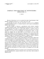
Remark 3. To recover t he classical interpretation of S(n, k) in Corollary 2, we can apply
a simple bijection, say ϕ, in [7, Prop. 3]. Starting from a k-partition π = {B
1
, . . . , B
k
}
of [n], for each non-singleton block B
i
= {p
1
, p
2
, . . . , p
n
i
} with n
i
 2 elements p
1
< p
2
<
. . . < p
n
i
, we associate the subdiag onal quasi-permutatio n
Q
i

= {(p
n
i
, p
n
i−1
), (p
n
i−1
, p
n
i−2
), . . . , (p
2
, p
1
)}
with n
i
− 1 elements of [n] × [n]. Clearly, the union of all such Q
′
i
s is a subdiagonal
quasi-permutation of cardinality n − k. An example of the map ϕ is given in Figure 3.
the electronic journal of combinatorics 17 (2010), #R70 9
Figure 3: The subdiagonal quasi-permutation corresponding to a partition via the map ϕ
π = {{1, 4, 6}, {2, 5}, {3}} −→
Finally, we derive from Theorem 4 and (1.14) a new combinatorial interpretation for
the Legendre-Stirling numbers of the second kind. The correspondence between the two
models will be established in the next subsection.

Corollary 7. The integer LS(n, k) is the number of ordered pairs (Q
1
, Q
2
) of simply
hooked k-quasi-permutations of [n] such that pr
y
(Q
1
) = pr
y
(Q
2
).
Remark 4. We haven’t found an interpretation neither for the numbers d
(i)
n,k
in (2.2), nor
for the formulas expressed in (2.4), in terms of simply hooked quasi-permutations.
2.3 The link between the two models
We introduce a third interpretatio n which permits to make the connection easier between
the two previous models. Let Π
n,k
be the set of partitions of [n] in k non-empty blocks.
Definition 4. Let B
(i)
n,k
be the set of triples (π
1
, π

2
, π
3
) in Π
n,k+i
× Π
n,k+i
× Π
n,n−i
such
that:
i) min(π
1
) = min(π
2
) and Sing(π
1
) = Sing(π
2
),
ii) min(π
1
) ∪ Sing(π
3
) = Sing(π
1
) ∪ min(π
3
) = [n],
where Sing(π) denotes the set of singletons in π.

We will need the following result.
Lemma 5. For (π
1
, π
2
, π
3
) ∈ B
(i)
n,k
, we have:
i) | min(π
1
) ∩ min(π
3
)| = k,
ii) |Sing(π
1
) \ min(π
3
)| = i,
iii) |Sing(π
3
) \ min(π
1
)| = n − k − i.
Proof. By definition, we have | min(π
1
)| = k + i and | min(π
3

)| = n − i. Since min(π
1
) ∪
min(π
3
) = [n], by sieve formula, we deduce
| min(π
1
) ∩ min(π
3
)| = | min(π
1
)| + | min(π
3
)| − | min(π
1
) ∪ min(π
3
)| = k,
and
|Sing(π
1
) \ min(π
3
)| = |Sing(π
1
)| − |Sing(π
1
) ∩ min(π
3

)| = n − | min(π
3
)| = i.
In the same way, we obtain iii).
the electronic journal of combinatorics 17 (2010), #R70 10
Theorem 6. There i s a b i jection between A
(i)
n,k
and B
(i)
n,k
.
Proof. Let π = {B
0
, B
1
, . . . , B
k
} be a signed k-partition in A
(i)
n,k
. We construct the triple
(π
1
, π
2
, π
3
) of partitions by the following a lgorithm.
π

1
, π
2
: • Let π
′
= {B
′
0
, B
′
1
, . . . , B
′
k
} be the partition obtained by exchanging all j and
−j in π if j ∈ B
0
(resp. j ∈ [n]).
• Let π
′′
= {B
′′
0
, B
′′
1
, . . . , B
′′
k
} be the partition obtained by removing all the

negative values in π
′
.
• Define π
1
(resp. π
2
) to be the partition obtained by splitting t he i positive
elements in B
′′
0
into i singletons and deleting 0 in π
′′
.
The resulting partitions π
1
and π
2
are clearly elements of Π
n,k+i
and satisfy
min(π
1
) = min(π
2
) and Sing(π
1
) = Sing(π
2
).

π
3
: • For all p ∈ [n] \ min π such that B
0
∩ {±p} = ∅, move p into the zero-block
and obtain the partition π
′
= {B
′
0
, B
′
1
, . . . , B
′
k
}. So there are n−k −i positive
entries in the new B
′
0
.
• Let π
′′
= {B
′′
0
, B
′′
1
, . . . , B

′′
k
} be the partition obtained by removing all the
negative values in π
′
.
• Define π
3
to be the partition obtained by splitting the n − k − i positive
elements in B
′′
0
into n − k − i singletons and deleting 0 in π
′′
.
The resulting partition π
3
is an element of Π
n,n−i
.
For any p ∈ [n] \ min(π
1
), if p /∈ B
0
then B
0
∩ {±p} = ∅, by definition p will be moved
in the zero-block, otherwise p is already in the zero- block. Thus, the elements that are
not in min(π
1

) become singletons in π
3
. Hence min(π
1
) ∪ Sing(π
3
) = [n]. Similarly we
have Sing(π
1
) ∪ min(π
3
) = [n].
For example, for the signed 3-partition of [±10]
0
:
π = {{−4, 6, 7, −8, −10}
0
, {±1, 3, 4, −5, −7}, {±2, −3, 5, −6, 8}, {±9, 10}}, (2.8)
the correspo nding tr iple is (π
1
, π
2
, π
3
) ∈ Π
10,6
× Π
10,6
× Π
10,7

with :
π
1
= {{1, 3, 7}, {2, 5, 6}, {4}, {8}, {9}, {10}},
π
2
= {{1, 5, 7}, {2, 3, 6}, {4}, {8}, {9}, {10}},
π
3
= {{1, 4}, {2, 8}, {3}, {5}, {6}, {7}, {9, 10}}.
(2.9)
Conversely, fo r any (π
1
, π
2
, π
3
) ∈ B
(i)
n,k
, we construct π = {B
0
, B
1
, . . . , B
k
} ∈ A
(i)
n,k
with

the following procedure:
• Use the k elements of min(π
1
) ∩ min(π
3
), say p
1
, . . . , p
k
and 0 to create k + 1 blocks:
B
0
= {. . .}
0
, B
1
= {±p
1
, . . .}, . . . , B
k
= {±p
k
. . .}, (2.10)
where “. . .” means that the blocks a r e not completed. For instance, for the triple
(π
1
, π
2
, π
3

) in (2.9), we create four blocks: {0, . . .}, {±1, . . .}, {±2, . . .} and {±9, . . .}.
the electronic journal of combinatorics 17 (2010), #R70 11
• For each element x
j
of [n] \ min(π
3
) (1  j  i), suppose that x
j
appears in a
non-singleton block C
j
of π
3
. Then put −x
j
into the zero-block B
0
and x
j
into the
block in ( 2.10) that contains min(C
j
). No te that we must show that min(C
j
) ∈
min(π
1
) ∩ min(π
3
) to warrant the existence of such a block in (2.10). Indeed, if

min(C
j
) /∈ min(π
1
), then, by Definition 4, we would have min(C
j
) ∈ Sing(π
3
). For
the current example, we place the number 4 in the block that contains 1.
• For each element y
j
of [n] \ min(π
2
) (1  j  n − k − i), suppose that y
j
appears in
a non-singleton block D
j
(resp. E
j
) of π
2
(resp. π
1
). Then put −p
j
into the block
in (2.10) that contains min(D
j

) and put p
j
into the block in (2 .1 0) that contains
min(E
j
) if this blo ck dosn’t contains −p
j
, into the zero-block B
0
otherwise. For the
current example, we place the number −3 in the block that contains 2. and 5 in
the block that contains 2, and 6 in the zero-block because the block that contains 2
already has −6.
Since ϕ described in Remark 3 maps each partition to a subdiagonal quasi-permutat io n,
for every triple (π
1
, π
2
, π
2
) of partitions satisfying the conditions of Theorem 6, we can
associate a triple (P
1
, P
2
, P
3
) = (ϕ (π
1
), ϕ(π

2
), ϕ(π
3
)) of subdiagonal quasi-permutations.
If P
i
denotes the supdiagonal quasi-permutatio n obtained from P
i
exchanging the x and y
coordonates, then (Q
1
, Q
2
) = (P
1
∪ P
3
, P
2
∪ P
3
) is an ordered pair of simply hooked quasi-
permutations satisfying the conditions of Theorem 4. Thus, we obtain a bijection between
the signed k-partitions and the ordered pairs of simply hooked quasi-permutations.
For example, for the signed 3-partition π in (2.8), the corresponding ordered pair of
simply hooked quasi-permutations (Q
1
, Q
2
) is then given by (2.6) (cf. Figure 2).

3 Jacobi-Stirling numbers of the first kind js
k
n
(z)
For a permutation σ of [n]
0
:= [n] ∪ {0} (resp. [n]) and for j ∈ [n]
0
(resp. [n]), denote by
Orb
σ
(j) = {σ
ℓ
(j) : ℓ  1} the orbit of j and min(σ) the set of its cyclic minima, i.e.,
min(σ) = {j ∈ [n] : j = min(Orb
σ
(j) ∩ [n])}.
Definition 5. Given a word w = w(1) . . .w(ℓ) on the finite a lphabet [n], a letter w(j) is
a record of w if w(k) > w(j) for every k ∈ {1, . . . , j − 1}. We define rec(w) to be the
number of records o f w and rec
0
(w) = rec(w ) − 1.
For example, if w = 5748623 19 , then the records are 5, 4, 2, 1. Hence rec(w) = 4.
Theorem 7. The integer b
(i)
n,k
is the number of ordered pairs (σ, τ) such that σ (resp. τ )
is a permutation of [n]
0
(resp. [n]) with k cycles, satisfying

i) 1 ∈ Orb
σ
(0),
ii) min σ = min τ ,
iii) rec
0
(w) = i, whe re w = σ(0)σ
2
(0) . . . σ
l
(0) with σ
l+1
(0) = 0.
the electronic journal of combinatorics 17 (2010), #R70 12
Proof. Let E
(i)
n,k
be the set of ordered pairs (σ, τ) satisfying the conditions of Theorem 7
and e
(i)
n,k
=



E
(i)
n,k




. We divide E
(i)
n,k
into three parts:
(i) the ordered pairs (σ, τ) such that σ
−1
(n) = n. Then n forms a cycle in both σ and
τ and there are clearly e
(i)
n−1,k−1
possibilities.
(ii) the ordered pairs (σ, τ) such that σ
−1
(n) = 0. We can construct such ordered pairs
by first choosing an ordered pair (σ
′
, τ
′
) in E
(i−1)
n−1,k
and then inserting n in σ
′
as image
of 0 (resp. in τ
′
). Clearly, there are (n − 1)e
(i−1)
n−1,k

possibilities.
(iii) the ordered pairs (σ, τ ) such that σ
−1
(n) ∈ {0, n}. We can construct such ordered
pairs by first choosing an ordered pair (σ
′
, τ
′
) in E
(i)
n−1,k
and then inserting n in σ
′
(resp. in τ
′
). Clearly, there are (n − 1 )
2
e
(i)
n−1,k
possibilities.
Summing up, we get the following equation:
e
(i)
n,k
= e
(i)
n−1,k−1
+ (n − 1)e
(i−1)

n−1,k
+ (n − 1)
2
e
(i)
n−1,k
. (3.1)
By (1.5), it is easy to see that the coefficients b
(i)
n,k
satisfy the same recurrence.
We show now how to derive from Theorems 1 and 7 the combinatorial interpretations
for the numbers |ls(n, k)|, |s(n, k)| and |u(n, k)|.
Corollary 8. The integer |ls(n, k)| is the number of ordered pairs (σ, τ) such that σ
(resp. τ) is a permutation of [n]
0
(resp. [n]) with k cycles, satisfying 1 ∈ Orb
σ
(0) and
min σ = min τ.
Corollary 9. The integer |s(n, k)| is the number of permutations of [n] with k cycles.
Proof. By Theorem 7, the integer |s(n, k)| is the number of ordered pairs (σ, τ) in E
(n−k )
n,k
.
Since σ and τ both have k cycles with same cyclic minima, the permutation σ is completely
determinated by τ because Orb
σ
(1) is the only non singleton cycle, of cardinality n−k+2,
so the n−k elements different from 0 and 1 are exactly the elements of [n]\min τ arranged

in decreasing order in the word w = σ(0)σ
2
(0) . . . 1 with σ(1) = 0.
The following result is the analogue interpretation to Corollary 3 for the central facto-
rial numbers of the first kind. This analogy is comparable with that of Stirling numbers
of the first kind |s(n, k)| versus the Stirling numbers of the second kind |S(n, k)|.
Corollary 10. The integer |u(n, k)| is the number of ordered pairs (σ, τ) ∈ S
2
n
with k
cycles, such that min(σ) = min(τ).
Indeed, the integer |u(n, k)| is the number of ordered pairs (σ, τ) in E
(0)
n,k
. Theorem 7
implies that σ
−1
(1) = 0. The result follows then by deleting the zero in σ.
Remark 5. By the substitution i → n + 1 − i, we can derive that the number |u(n, k)| is
also the number of ordered pairs (σ, τ) in S
2
n
with k cycles, such that max(σ) = max(τ),
where max(σ) is the set of cyclic maxima of σ, i.e.,
max(σ) = {j ∈ [n] : j = max(Orb
σ
(j)}.
the electronic journal of combinatorics 17 (2010), #R70 13
Table 4: The first values of V (n, k) and |v(n, k)|
k\n 0 1 2 3 4 5

0 1 1 1 1 1 1
1 1 10 91 820 7381
2 1 35 966 24970
3 1 84 5082
4 1 165
5 1
k\n 0 1 2 3 4 5
0 1 1 9 225 11025 893025
1 1 10 259 12916 1057221
2 1 35 1974 172810
3 1 84 8778
4 1 165
5 1
4 Further results
4.1 Central factorial numbers of odd ind ices
For all n, k  0, set
V (n, k) = 4
n−k
T (2n + 1, 2k + 1), v(n, k) = 4
n−k
t(2n + 1, 2k + 1).
Note that these numbers are also integers (see Table 4). By definition, we have the
following recurrence relations :
V (n, k) = V (n − 1, k − 1) + (2k + 1)
2
V (n − 1, k) , (4.1)
v(n, k) = v(n − 1 , k − 1) − ( 2n − 1)
2
v(n − 1, k). (4.2)
The natural question is to find a combinato r ia l interpretation for these numbers. We

can easily find it from combinatorial theory of generating functions.
Theorem 8. The integer V (n, k) is the number of partitions of [2n+1] into 2k +1 blocks
of odd cardinality.
Proof. This follows from the known generating function (see [8, p. 214]):

n,k0
V (n, k)t
k
x
n
n!
= sinh(t sinh(x)),
and the classical combinatorial theory of generating functions (see [7, Chp. 3] and [9,
Chp. 5 ]).
To interpret the integer |v(n, k)|, we need to introduce the following definition.
Definition 6. A (n, k)-Riordan complex is a (2k + 1)-tuple
((B
1
, σ
1
, τ
1
), . . . , (B
2k+1
, σ
2k+1
, τ
2k+1
))
such that

the electronic journal of combinatorics 17 (2010), #R70 14
i) {B
1
, . . . , B
2k+1
} is a partition of [2n + 1] into blocks B
i
of odd cardinality;
ii) σ
i
and τ
i
(1  i  2k + 1) are fixed point free involutions on B
i
\ max(B
i
).
Theorem 9. The integer |v(n, k)| is the number of (n, k)-Riordan complexes.
Proof. It is known that (see [8, p. 214]):

n,k0
|v(n, k ) |t
k
x
n
n!
= sinh(t arcsin(x)),
and
arcsin(x) =


n0
((2n − 1)!!)
2
x
2n+1
(2n + 1)!
,
where (2n − 1)!! = (2n − 1)(2n − 3) · · · 3 · 1. Since (2n − 1)!! is the number of involutions
without fixed points on [2n] (see [2]), the integer ((2n − 1)!!)
2
is the number o f ordered
pairs of involutions without fixed points on [2n + 1]\{2n + 1}.
Define the numbers J(n, m) by:
exp

t

n1
((2n − 1)!!)
2
x
2n+1
(2n + 1)!

=

n,m0
J(2n + 1, m)t
m
x

2n+1
(2n + 1)!
.
Then, by the theory of exponential generating functions (see [7, Chp. 3] and [9, Chp. 5]),
the coefficient J(2n + 1, m) is the number of m-tuples
(B
1
, σ
1
, τ
1
), . . . , (B
m
, σ
m
, τ
m
);
where {B
1
, . . . , B
m
} is a partition of [2n + 1] with |B
i
| odd (1  i  m), and σ
i
and τ
i
are involutions without fixed po ints on B
i

\ max(B
i
). As sinh(x) = (e
x
− e
−x
)/2, we have
|v(n, m)| = J(2n + 1, 2k + 1) if m = 2k + 1, and |v(n, m)| = 0 if m is even.
Remark 6. From (1.9), we can easily deduce that
n

k=0
|v(n, k ) |t
2k+1
= t(t
2
+ 1)(t
2
+ 3
2
) . . . (t
2
+ (2n − 1)
2
). (4.3)
It is interesting to note that a proof of the latter result is not obvious from (4.3). In the
same way, proofs for Theorems 8 and 9 by using (4.1) or (4.2) are not obvious.
Example 1. There are ten (2, 1)-Riordan complexes. Since the numbers n and k are
small, the involved involutions are identical transpositions.
{1}, {(2, 3), 4}, {5}, {1}, {2}, {(3, 4), 5},

{(1, 2), 3}, {4}, {5}, {(1, 2), 5}, {3}, {4},
{(1, 3), 4}, {2}, {5}, {(1, 3), 5}, {2}, {4},
{(1, 2), 4}, {3}, {5}, {(1, 4), 5}, {2}, {3},
{1}, {(2, 3), 5}, {4}, {1}, {(2, 4), 5}, {3},
where {1}, {(2, 3), 4}, {5} means that π = {{1}, {2, 3, 4}, {5}}, and σ = τ = 13245.
the electronic journal of combinatorics 17 (2010), #R70 15
4.2 Generating functions
In [5], the authors made a long calculation to derive an explicit fo rmula for the Jacobi-
Stirling numbers. Actually, we can derive an explicit formula for the Jacobi-Stirling
numbers straightforwardly from the Newton interpolation formula:
x
n
=
n

j=0




j

r=0
x
n
r

k=i
(x
r

− x
k
)




j−1

i=0
(x − x
i
). (4.4)
Indeed, making the substitutions x → m(z + m) and x
i
→ i(z + i) in (4.4), we o bta in
(m(m + z))
n
=
n

j=0
JS
j
n
(z)(m − j + 1)
j
(z + m)
j
, (4.5)

where
JS
j
n
(z) =
j

r=0
(−1)
r
[r(r + z)]
n
r!(j − r)!(z + r)
r
(z + 2r + 1)
j−r
, (4.6)
and (z)
n
= z(z + 1 ) . . .(z + n − 1).
Remark 7. If we substitute x by m(m + z) + k, we obtain [5, Theorem 4.1].
From the recurrence (1.4), we derive:

nk
JS
k
n
(z)x
n
=

x
1 − k(k + z)

nk− 1
JS
k−1
n
(z)x
n
; (4.7)
therefore,

nk
JS
k
n
(z)x
n
=
x
k
(1 − (z + 1)x)(1 − 2(z + 2)x) . . . (1 − k(z + k)x)
. (4.8)
Acknowledg ement
This work was partially supported by the French National Research Agency through the
grant ANR-08-BLAN-0243-03.
References
[1] G. E. Andrews, L. L. Littlejohn, A combinatorial interpretation of the Legendre-
Stirling numbers, Proc. Amer. Math. Soc. 137 (2009), 2581-2590.
[2] L. Comtet, Advanced combinatorics, Boston, Dordrecht, 1974.

the electronic journal of combinatorics 17 (2010), #R70 16
[3] D. Dumont, Interpr´etations combinatoires des nombres de Genocchi, Duke Math. J.,
t. 41, 1974, p. 305-318.
[4] W. N. Everitt, L. L. Littlejohn, R. Wellman, Legendre polynomials, Legendre-Stirling
numbers, and the l eft-definite spectral analysis of the Legendre differential expression,
J. Combut. Appl. Math., 148 (2002), 213-23 8.
[5] W. N. Everitt, K. H. Kwon, L. L. Littlejohn, R. Wellman, G. J. Yoon, Jacobi-
Stirling numbers, Jacobi polynomials, and the left-definite analysis of the classical
Jacobi differential expression, J. Combut. Appl. Math., 208 (2007), 29-56.
[6] D. Foata, G. -N. Han, Princi pes de comb i natoire classique, Lecture notes, Strasbourg,
2000, revised 200 8.
[7] D. Foata, M. P. Sch¨utzenberger, Th´eorie g´eom´etrique des polynˆomes eul´eriens, Lec-
ture Notes in Math no. 138, Springer-Verlag, Berlin, 1970.
[8] J. Riordan, Combinatorial Identities, John Wiley & Sons, Inc., 1968.
[9] R. P. Stanley, Enumerative Combinatorics, vo l . 2, Cambridge Studies in Advanced
Mathematics, 62, 1999.
the electronic journal of combinatorics 17 (2010), #R70 17