Báo cáo toán học: "A conjecture of Biggs concerning the resistance of a distance-regular graph" potx
Bạn đang xem bản rút gọn của tài liệu. Xem và tải ngay bản đầy đủ của tài liệu tại đây (253.37 KB, 15 trang )
A conjecture of Biggs concerning the resistance
of a distance-regular graph
Greg Markowsky Jacobus Koolen
jacobus
Pohang Mathematics Institute Department of Mathematics
POSTECH POSTECH
Pohang, 790-784 Pohang, 790-784
Republic of Korea Republic of Korea
Submitted: Apr 12, 2010; Accepted: May 18, 2010; Published: May 25, 2010
Mathematics Subject Classification: 05E30
Abstract
Biggs conjectured that the resistance between any two points on a distance-
regular graph of valency greater than 2 is bounded by twice the resistance between
adjacent points. We prove this conjecture, give the sharp constant for the inequality,
and display the graphs for which the conjecture most nearly fails. Some neces sary
background material is included, as well as some consequences.
1 Introduction
The main goal of this paper is to prove the following conjecture of Biggs:
Theorem 1 Let G be a distance-regular graph with degree larger than 2 and diameter D.
If d
j
is the electric resistance between any two vertices of distance j, then
max
j
d
j
= d
D
Kd
1
(1)
where K = 1 +
94
101
≈ 1.931. Equality holds only in the case of the Biggs-Smith graph.
We remark that for degree 2 the theorem is trivially false. This theorem implies several
statements concerning random walks on distance-regular graphs, which will be given at
the end of the paper. General background material on the concept of electric resistance,
as well as its connection to random walks, can be found in the excellent references [6]
and [2]. Biggs’ conjecture originally appeared in [1], which discusses electric resistance
on distance-regular graphs only. To understand the proof of the conjecture, one must
the electronic journal of combinatorics 17 (2010), #R78 1
understand much of the material in [1]. We have therefore decided to include the material
from [1] which is key to Theorem 1. This appears in Section 3, following the relevant
graph-theoretic definitions in Section 2. Section 4 gives our proof of the theorem, and
Section 5 gives some consequences, including several in the field of random walks.
2 Distance-regular graphs
All the graphs considered in this paper are finite, undirected and simple (for unexplained
terminology and more details, see for example [4]). Let G be a connected graph and let
V = V (G) be the vertex set of G. The distance d(x, y) between any two vertices x, y of G
is the length of a shortest path between x and y in G. The diameter of G is the maximal
distance occurring in G and we will denote this by D = D(G). For a vertex x ∈ V (G),
define K
i
(x) to be the set of vertices which are at distance i from x (0 i D) where
D := max{d(x, y) | x, y ∈ V (G)} is the diameter of G. In addition, define K
−1
(x) := ∅
and K
D+1
(x) := ∅. We write x ∼
G
y or simply x ∼ y if two vertices x and y are adjacent
in G. A connected graph G with diameter D is c alled distance-regular if there are integers
b
i
, c
i
(0 i D) such that for any two vertices x, y ∈ V (G) with d(x, y) = i, there are
precisely c
i
neighbors of y in K
i−1
(x) and b
i
neighbors of y in K
i+1
(x) (cf. [4, p.126]).
In particular, distance-regular graph G is regular with valency k := b
0
and we define
a
i
:= k − b
i
− c
i
for notational convenience. The numbers a
i
, b
i
and c
i
(0 i D) are
called the intersection numbers of G. Note that b
D
= c
0
= a
0
= 0, b
0
= k and c
1
= 1.
The intersection numbers of a distance-regular graph G with diameter D and valency k
satisfy (cf. [4, Proposition 4.1.6])
(i) k = b
0
> b
1
· · · b
D−1
;
(ii) 1 = c
1
c
2
· · · c
D
;
(iii) b
i
c
j
if i + j D.
Moreover, if we fix a vertex x of G, then |K
i
| does not depend on the choice of x as
c
i+1
|K
i+1
| = b
i
|K
i
| holds for i = 1, 2, . . . D − 1. In the next section, it will be shown that
the resistance between any two vertices of G can be calculated explicitly using only the
intersection array, so that the proof can be conducted using only the known properties of
the array.
3 Electric resistance on distance-regular graphs
Henceforth let G be a distance-regular graph with n vertices, degree k 3, and diameter
D. Let V = V (G) and E = E(G) be the vertex and edge sets, respectively, of G. To
calculate the resistance between any two vertices we use Ohm’s Law, which states that
V = IR(2)
the electronic journal of combinatorics 17 (2010), #R78 2
where V represents a difference in voltage(or potential), I represents current, and R
represents resistance. That is, we imagine that our graph is a circuit where each edge
is a wire with resistance 1. We attach a battery of voltage V to two distinct vertices u
and v, producing a current through the graph. The resistance between the u and v is
then V divided by the current produced. The current flowing through the circuit can
be determined by calculating the voltage at each point on the graph, then summing the
currents flowing from u, say, to all vertices adjacent to u. Calculating the voltage at each
point is thereby seen to be an important problem. A function f on V is harmonic at a
point z ∈ V if f(z) is the average of neighboring values of f, that is
x∼z
(f(x) − f(z)) = 0(3)
The voltage function on V can be characterized as the unique function which is harmonic
on V − {u, v} having the prescribed values on u and v. For our purposes, on the distance-
regular graph G, we will first supp ose that u and v are adjacent. It is easy to see that,
for any vertex z, |d(u, z) − d(v, z)| 1, where d denotes the ordinary graph-theoretic
distance. Thus, any z must be contained in a unique set of one of the following forms:
K
i
i
= {x : d(u, x) = i and d(v, x) = i}(4)
K
i+1
i
= {x : d(u, x) = i + 1 and d(v, x) = i}
K
i
i+1
= {x : d(u, x) = i and d(v, x) = i + 1}
Suppose that (b
0
, b
1
, . . . , b
D−1
; c
1
, c
2
, . . . , c
D
) is the intersection array of G. For 0 i
D − 1 define the numbers φ
i
recursively by
φ
0
= n − 1(5)
φ
i
=
c
i
φ
i−1
− k
b
i
We then have the following fundamental proposition.
Proposition 1 The function f defined on V by
f(u) = −f(v) = φ
0
(6)
f(z) = 0 for x ∈ K
i
i
f(z) = φ
i
for x ∈ K
i
i+1
f(z) = −φ
i
for x ∈ K
i+1
i
is harmonic on V − {u, v}.
In the following intersection diagram, the value of f on each set is given directly outside
the set.
the electronic journal of combinatorics 17 (2010), #R78 3
Figure 1
To prove Proposition 1 we need the following lemma, which may be of interest in its own
right.
Lemma 1 Let z ∈ G, and let K
i
= {x : d(z, x) = i} as in Section 2. Let e
i
be the number
of edges of G with one endpoint in K
i
and the other in K
i+1
. Then
φ
i
=
k
j>i
|K
j
|
e
i
(7)
Proof: Since φ
0
= n − 1 =
j>0
|K
j
| and e
0
= k, it is clear that (7) holds for i = 0. We
need therefore only verify that the numbers ψ
i
=
k
P
j>i
|K
j
|
e
i
satisfy the recursive relation
given in (5). This is immediate from the facts that e
i
= b
i
|K
i
| and e
i−1
= c
i
|K
i
|, for we
see that
c
i
ψ
i−1
− k
b
i
=
c
i
(
k|K
i
|+k
P
j>i
|K
j
|
e
i−1
) − k
b
i
(8)
=
c
i
k
j>i
|K
j
|
b
i
e
i−1
=
k
j>i
|K
j
|
b
i
K
i
=
k
j>i
|K
j
|
e
i
= ψ
i
the electronic journal of combinatorics 17 (2010), #R78 4
Proof of Proposition 1: Suppose first that z ∈ K
i
i
for some i. The points adjacent to z
must lie within K
i
i
K
i−1
i−1
K
i+1
i+1
K
i+1
i
K
i−1
i
K
i
i−1
K
i
i+1
. Since b
i
is equal to the
number of adjacent points in K
i+1
i+1
K
i+1
i
, and also in the set K
i+1
i+1
K
i
i+1
, we see that
|{x : z ∼ x and x ∈ K
i
i+1
}| = |{x : z ∼ x and x ∈ K
i+1
i
}|(9)
A similar argument shows
|{x : z ∼ x and x ∈ K
i
i−1
}| = |{x : z ∼ x and x ∈ K
i−1
i
}|(10)
It follows from this that
x∼z
f(x) = 0 = f(z)(11)
and f is harmonic at z. Now suppose that z ∈ K
i
i+1
with 1 i D − 2. Here the points
adjacent to z must lie within K
i
i+1
K
i−1
i
K
i+1
i+2
K
i
i
K
i+1
i+1
K
i+1
i
. The number of
edges from z to points in K
i−1
i
is c
i
and to points in K
i+1
i+2
is b
i+1
. Let the number of edges
from z to points in K
i+1
i
be α. Then the number of edges from z to other points in K
i
i+1
is given by k + α − c
i+1
− b
i
. We therefore have
x∼z
f(x) = b
i+1
φ
i+1
+ c
i
φ
i−1
+ (k + α − c
i+1
− b
i
)φ
i
+ α(−φ
i
)(12)
= kφ
i
= kf(z)
where we have used the following equations equivalent to the recursive relation in (5).
c
i
φ
i−1
= b
i
φ
i
+ k(13)
b
i+1
φ
i+1
= c
i+1
φ
i
− k
We see that f is harmonic at z. The same argument works for z ∈ K
D−1
D
, except that there
is some difficulty in using the last equation in (13), as b
D
= 0, and φ
i
was only defined
for i D − 1. Happily, Lemma 1 solves our dilemma, for as an immediate consequence
we obtain φ
D−1
=
k
c
D
. Thus, defining φ
D
= 0 is consistent with (13), and f is harmonic
on K
D−1
D
. By symmetry, f is harmonic at all points lying in sets of the form K
i
i+1
, and
the proof is complete.
Corollary 1. φ
i
> φ
i+1
for 0 i D − 2
Proof: Suppose φ
i
φ
i+1
for some i. Due to the monotonicity of the sequences b
i
, c
i
, we
would have
φ
i+2
=
c
i+2
φ
i+1
− k
b
i+2
c
i+1
φ
i
− k
b
i+1
= φ
i+1
(14)
Continuing in this way we would have φ
D−1
φ
D−2
. On the other hand, by harmonicity
φ
D−1
is the weighted average of the values φ
D−2
, 0, and −φ
D−1
, so that φ
D−1
< φ
D−2
.
This is a contradiction.
the electronic journal of combinatorics 17 (2010), #R78 5
It may interest the reader to note that the subtracted constant k in the numerator of the
recursive relation of (5) can be replaced by any constant without affecting harmonicity
outside of the sets K
D−1
D
and K
D
D−1
. However, k is the only constant which gives φ
D
= 0,
and therefore is the constant dictated by the requirement that f be harmonic and attain
the boundary values of (n − 1) and −(n − 1) at u and v. The resistance between u and v
can now easily be computed as the voltage difference between the points, 2φ
0
= 2(n − 1),
divided by the current I flowing through the circuit. This current is the sum of the voltage
differences between u and vertices adjacent to u, and is readily computable as I = nk.
We see that the resistance between u and v is
R
uv
=
2(n − 1)
nk
=
n − 1
m
(15)
where m = nk/2 is the number of edges in G. This result is in fact an immediate conse-
quence of Foster’s Network Theorem(see [2] or [7]), and was derived, among other things,
by other methods in [10]. In the remainder of this section, however, it will be more con-
ceptually convenient to keep I and the φ’s in the formulas rather than their explicit values,
as this reminds us that they represent the current and voltages, respectively. Calculating
the resistances between nonadjacent vertices might now seem to be a formidable task, but
in fact there is virtually no more to be done. We have the following proposition.
Proposition 2 The resistance between two vertices of distance j in a graph is given by
2
0i<j
φ
i
I
(16)
Proof: Suppose d(u, v) = j. We can choose points x
0
= u, x
1
, . . . , x
j
= v such that
x
i
∼ x
i+1
. For any pair of adjacent points y, z we let f
yz
be the unique func tion on V given
in Proposition 1 which is harmonic on V − {y, z} and which satisfies f(w) = −f(z) = φ
0
.
The key claim is that for any three points w, y, z with y ∼ w ∼ z the function f
yw
+ f
wz
is harmonic on V − {y, z}. This is clear for all points in V − {y, z} except w. To show
harmonicity at w, note that a current of I flows into w due to f
yw
, whereas a current of I
flows out of w due to f
wz
. The net current flow into w is therefore 0, which is equivalent to
harmonicity(see [6]). Thus, the voltage function g =
0ij−1
f
x
i
x
i+1
, which is harmonic
on V −{u, v}, gives rise to a current of I flowing from u to v. We must therefore calculate
the values of the function g at the points u and v. It is straightforward to verify that
f
x
i
x
i+1
(u) = φ
i
(since u lies in the set K
i
i+1
formed with respect to the pair x
i
, x
i+1
), and
likewise f
x
i
x
i+1
(v) = −φ
D−(i+1)
. Thus, g(u) =
0i<j
φ
i
and g(v) = −
0i<j
φ
i
. The
result follows.
4 Proof of Theorem
In fact, we will prove a statement stronger than Theorem 1. Let E be the set of the
following four graphs, with corresponding properties listed:
the electronic journal of combinatorics 17 (2010), #R78 6
Name
1
Vertices Intersection array
φ
1
+ +φ
D−1
φ
0
Biggs-Smith Graph 102 (3,2,2,2,1,1,1;1,1,1,1,1,1,3) 0.930693
Foster Graph 90 (3,2,2,2,2,1,1,1;1,1,1,1,2,2,2,3) 0.896067
Flag graph of GH(2,2) 189 (4,2,2,2,2,2;1,1,1,1,1,2) 0.882979
Tutte’s 12-Cage 126 (3,2,2,2,2,2;1,1,1,1,1,3) 0.872
Theorem 2 Other than graphs in E, for any distance regular graph with degree at least
3 we have
φ
1
+ . . . + φ
D−1
< .87φ
0
(17)
This clearly implies The orem 1 and shows that the graphs in E are the extremal cases.
Proof of Theo rem 2: The proof proceeds by considering a number of separate cases,
and leans heavily on the standard reference [4]. Without access to this book, the proof
will likely be incomprehensible to the reader. In the estimates used in the proof, the −k
in the numerator of the recurrence relation is largely ignored, but the reader should be
warned that this term is by no means unnecessary. That is because it is crucial that the
φ
i
’s form a monotone decreasing sequence, and without the −k this would not be the case.
Nevertheless, we will from this point forth mainly use the facts φ
i
<
c
i
φ
i−1
b
i
and φ
i
< φ
i−1
.
We are required to show
φ
1
+ . . . + φ
D−1
φ
0
.87(18)
for all graphs not in E.
Case 1 : D = 2.
We need only s how φ
1
< .87φ
0
. This is clear if b
1
> 1, since c
1
= 1 and φ
i
<
c
i
φ
i−1
b
i
. The
case b
1
= 1 is known to occur only in the case of the Cocktail party graphs, and it is
simple to verify the relation in this case.
Case 2 : k = 3.
It is known(see [4], Theorem 7.5.1) that the only distance-regular graphs of degree 3 with
diameter greater than 2 are given by the intersection arrays below, and which give rise to
the resistances given:
1
The referee has pointed out that Tutte’s 12-Cage may be more accurately referred to as Benson’s
graph, and indeed the literature is mixed on this point. The referee further remarked that the Flag graph
of GH (2,2) can also be realized as the line graph of Tutte’s 12-Cage, or Benson’s graph. In this table,
we are employing the names given in [4].
the electronic journal of combinatorics 17 (2010), #R78 7
Name Vertices Intersection array
φ
1
+ φ
D−1
φ
0
Cube 8 (3,2,1;1,2,3) 0.428571
Heawood graph 14 (3,2,2;1,1,3) 0.461538
Pappus graph 18 (3,2,2,1;1,1,2,3) 0.588235
Coxeter graph 28 (3,2,2,1;1,1,1,2) 0.666667
Tutte’s 8-cage 30 (3,2,2,2;1,1,1,3) 0.655172
Dodecahedron 20 (3,2,1,1,1;1,1,1,2,3) 0.842105
Desargues graph 20 (3,2,2,1,1;1,1,2,2,3) 0.710526
Tutte’s 12-cage 126 (3,2,2,2,2,2;1,1,1,1,1,3) 0.872
Biggs-Smith graph 102 (3,2,2,2,1,1,1;1,1,1,1,1,1,3) 0.930693
Foster graph 90 (3,2,2,2,2,1,1,1;1,1,1,1,2,2,2,3) 0.896067
Case 3 : k = 4.
It is known(see [3]) that the only distance-regular graphs of degree 4 with diameter greater
than 2 are given by the intersection arrays below, and which give rise to the resistances
given:
Name Vertices Intersection array
φ
1
+ φ
D−1
φ
0
K
5,5
minus a matching 10 (4,3,1;1,3,4) 0.296296
Nonincidence graph of P G(2, 2) 14 (4,3,2;1,2,4) 0.307692
Line graph of Petersen graph 15 (4,2,1;1,1,4) 0.428571
4-cube 16 (4,3,2,1;1,2,3,4) 0.422222
Flag graph of P G(2, 2) 21 (4,2,2;1,1,2) 0.5
Incidence graph of P G(2, 3) 26 (4,3,3;1,1,4) 0.32
Incidence graph of AG(2, 4)-p.c. 32 (4,3,3,1;1,1,3,4) 0.376344
Odd graph O
4
35 (4,3,3;1,1,2) 0.352941
Flag graph of GQ(2, 2) 45 (4,2,2,2;1,1,1,2) 0.681818
Doubled odd graph 70 (4,3,3,2,2,1,1;1,1,2,2,3,3,4) 0.521739
Incidence graph of GQ(3, 3) 80 (4,3,3,3;1,1,1,4) 0.417722
Flag graph of GH(2, 2) 189 (4,2,2,2,2,2;1,1,1,1,1,2) 0.882979
Incidence graph of GH(3, 3) 728 (4,3,3,3,3,3;1,1,1,1,1,4) 0.485557
Case 4 : D 5, b
1
5.
This case was done initially by Biggs in [1], without the restriction on b
1
but with the
constant 1 in place of .87. Nevertheless, when we restrict b
1
as above this is trivial, because
φ
1
φ
0
<
1
b
1
and φ
i
φ
1
for all i > 0. Therefore,
φ
1
+ . . . + φ
D−1
φ
0
(D − 1)φ
1
φ
0
4
b
1
.8(19)
Henceforth, in all cases for which b
1
5 we can assume D 6. In what follows, let j
denote the smallest value such that c
j
b
j
. If c
j
> b
j
, then, since c
D−j
b
j
and the c
i
’s
are nondecreasing, we see that D − j < j, hence D 2j − 1. If c
j
= b
j
, then it follows
the electronic journal of combinatorics 17 (2010), #R78 8
from Corollary 5.9.6 of [4] that c
2j
> b
2j
. For this to occur, either c
2j
> b
j
or c
j
> b
2j
.
By the same argument as before, we obtain D 3j − 1. This will be of fundamental
importance in our proof. To begin with, we see that when D 6 we must have j 3.
Case 5 : G is a line graph.
The distance-regular line graphs have been classified, and appear in Theorem 4.2.16 of
[4]. All such graphs with k 3 have D 2 and are therefore covered by Case 1, w ith two
exceptions. First of all, G may be a generalized 2D-gon of order (1, s). The intersection
array of G is then of the form (2(a
1
+ 1), a
1
+ 1, . . . , a
1
+ 1; 1, 1, . . . , 1, 2), with a
1
> 1. The
other possibility is that G could be the line graph of a Moore graph, and in this case the
intersection array of G is of the form (2κ − 2, κ − 1, κ − 2; 1, 1, 4), for some κ 3. In both
of these cases it is straightforward to verify that the conclusion of the theorem holds.
Case 6 : b
1
5, j = 3, c
2
= 1.
Since j = 3, b
2
2 and D 8. We have
φ
1
+ . . . + φ
D−1
φ
0
φ
1
+ 6φ
2
φ
0
1
b
1
+
6
2b
1
=
4
b
1
.8(20)
Case 7 : b
1
5, j = 3, c
2
> 1.
By Theorem 5.4.1 in [4], c
2
2
3
c
3
. If c
3
> b
3
then D 2j − 1 = 5, which was covered in
Case 4. If c
3
= b
3
b
2
, then if we assume
c
2
b
2
1
2
we have
φ
1
+ . . . + φ
D−1
φ
0
φ
1
+ 6φ
2
φ
0
1
b
1
+
3
b
1
=
4
b
1
.8(21)
On the other hand, if it is not the case that
c
2
b
2
1
2
, then the proof of Theorem 5.4.1 of
[4] implies that G contains a quadrangle. By Corollary 5.2.2 in [4], D
2k
k+1−b
1
. It is
straightforward to verify that the fact that k b
1
+ 1 implies that
2k
k + 1 − b
1
b
1
+ 1(22)
We therefore see that the fact that G contains a quadrangle implies D b
1
+ 1. Further-
more, we s till have
c
2
b
2
2
3
by Theorem 5.4.1 of [4]. We therefore have
φ
1
+ . . . + φ
D−1
φ
0
φ
1
+ (b
1
− 1)φ
2
φ
0
1
b
1
+
2(b
1
− 1)
3b
1
=
2b
1
+ 1
3b
1
.7(23)
Case 8 : b
1
5, j 4, c
2
= 1.
If j 4 and b
2
= 2 then we must have b
3
= 2, c
3
= 1, so that
b
2
b
3
c
2
c
3
= 4. On the other
hand, if this does not occur than
b
2
c
2
3. We will consider these cases separately.
the electronic journal of combinatorics 17 (2010), #R78 9
Subcase 1:
b
2
c
2
3.
For i < j we have b
1
b
i
> c
i
, and for any i with c
i
> 1 we must have b
i
< b
1
, by
Proposition 5.4.4 in [4]. Thus,
c
i
b
i
b
1
−2
b
1
−1
. Define α =
b
1
−2
b
1
−1
. We have
φ
1
+ . . . + φ
D−1
φ
0
1
b
1
+
1
3b
1
+
α
3b
1
+ . . . +
α
j−3
3b
1
+
(2j − 1)α
j−3
3b
1
(24)
Replace the second through (j − 1)th term by a geometric series to obtain
φ
1
+ . . . + φ
D−1
φ
0
<
1
b
1
+
1
3b
1
1
1 −
b
1
−2
b
1
−1
+
(2j − 1)α
j−3
3b
1
(25)
<
1
b
1
+
b
1
− 1
3b
1
+
2(j − 1/2)α
j−1/2
3b
1
α
5/2
Simple calculus shows that the maximum of the function uα
u
is
−1
e ln α
. We therefore obtain
φ
1
+ . . . + φ
D−1
φ
0
<
b
1
+ 2
3b
1
+
−2
3b
1
(
b
1
−2
b
1
−1
)
5/2
e ln(
b
1
−2
b
1
−1
)
(26)
It is straightforward to verify that the function (b−2) ln(
b−2
b−1
) is increasing in b, so that the
right hand side of (26) achieves its maximum on the allowed range when b
1
= 5. Plugging
in b
1
= 5 gives approximately .851 as a bound for (26).
Subcase 2:
b
2
b
3
c
2
c
3
4.
This follows much as in the previous case, except that we may simplify by using the
slightly weaker bound
c
i
b
i
b
1
−1
b
1
for i < j. Let α =
b
1
−1
b
1
. Since b
2
b
3
and c
2
c
3
we
must have
b
2
c
2
2. We then have
φ
1
+ . . . + φ
D−1
φ
0
1
b
1
+
1
2b
1
+
1
4b
1
+
α
4b
1
+. . .+
α
j−3
4b
1
+
(2j − 1)α
j−3
4b
1
(27)
Following the steps in (31) above, we obtain
φ
1
+ . . . + φ
D−1
φ
0
<
3
2b
1
+
1
4
+
−1
2b
1
(
b
1
−1
b
1
)
5/2
e ln(
b
1
−1
b
1
)
(28)
Again this is decreasing in b
1
, and plugging in b
1
= 5 gives a bound for (28) of about .84.
Case 9 : b
1
3, j 4, c
2
> 1, G contains a quadrangle.
As in the argument given in Case 7, we see that G containing a quadrangle implies
D b
1
+ 1. Furthermore, Theorem 5.4.1 of [4] implies that c
3
(3/2)c
2
. Since j 4 and
thus b
2
b
3
> c
3
we must have
c
2
b
2
2
3
. This gives
φ
1
+ . . . + φ
D−1
φ
0
1
b
1
+ (b
1
− 1)
2
3b
1
=
2b
1
+ 1
3b
1
(29)
the electronic journal of combinatorics 17 (2010), #R78 10
When b
1
3 this is bounded by .8.
Case 10 : b
1
3, j 4, c
2
1, G does not contain a quadrangle.
In this case G is a Terwilliger graph. By Corollary 1.16.6 of [4], if k < 50(c
2
− 1) then
D 4 and b
1
5, which was covered in Case 4. Thus, we can assume k 50(c
2
− 1),
which implies b
1
10c
2
. If b
2
3c
2
then we can follow the proof of Subcase 1 of Case 8
to obtain our result, so we may assume b
2
3c
2
, which implies b
2
<
b
2
. It follows from
this that for i < j
c
2
b
2
(b
1
/2)−1
b
1
/2
=
b
1
−2
b
1
. We set α =
b
1
−2
b
1
. By the proof of Theorem 5.4.1
in [4] we have c
3
2c
2
. Since b
2
b
3
> c
3
2c
2
we have
b
2
c
2
2. We compute
φ
1
+ . . . + φ
D−1
φ
0
1
b
1
+
1
2b
1
+
α
2b
1
+ . . . +
α
j−3
2b
1
+
(2j − 1)α
j−3
2b
1
(30)
Replace the second through (j − 1)th term by a geometric series to obtain
φ
1
+ . . . φ
D−1
φ
0
<
1
b
1
+
1
2b
1
1
1 −
b
1
−2
b
1
+
(2j − 1)α
j−3
2b
1
(31)
<
1
b
1
+
1
4
+
(j − 1/2)α
j−1/2
b
1
α
5/2
The maximum of the function uα
u
is
−1
e ln α
. We therefore obtain
φ
1
+ . . . φ
D−1
φ
0
<
1
b
1
+
1
4
+
−1
b
1
(
b
1
−2
b
1
)
5/2
e ln(
b
1
−2
b
1
)
(32)
As before, the function (b − 2) ln(
b−2
b
) is increasing in b, so the right hand side of (32) is
decreasing in b
1
. Plugging in b
1
= 10(recall that b
1
10c
2
10) gives approximately .64
as a bound.
Case 11 b
1
= 3 or 4, k 5, c
2
= 1.
This will be broken down into cases by degree k. Proposition 1.2.1 in [4] implies that
(a
1
+ 1)|k, so since b
1
= k − a
1
− 1 and b
1
> 0 we see that b
1
k/2. This implies k 8.
Subcase k = 8: b
1
= 3 is ruled out because (a
1
+ 1)|k. Suppose b
1
= 4. By Proposition
4.3.4 of [4], G is a line graph, and is therefore covered by Case 5.
Subcase k = 7: Since (a
1
+ 1)|k, we must have a
1
= 0 and thus b
1
= 6, which is a
contradiction.
Subcase k = 6: Since (a
1
+ 1)|k, we have a
1
∈ {0, 1, 2}. If a
1
= 0, then b
1
= 5, a
contradiction. If a
1
= 1, then as was shown in [9] G is one of the following graphs.
Name Vertices Intersection array
φ
1
+ φ
D−1
φ
0
Colinearity graph of GQ(2, 2) 15 (6,4;1,3) 0.142857
Colinearity graph of GH(2, 2) 27 (6,4,2;1,2,3) 0.269231
Hamming graph H(3, 3) 63 (6,4,4;1,1,3) 0.258065
Halved Foster graph 45 (6,4,2,1;1,1,4,6) 0.278409
the electronic journal of combinatorics 17 (2010), #R78 11
If a
1
= 2, then by Proposition 4.3.4 of [4], G is a line graph, and is therefore covered by
Case 5.
Subcase k = 5: Since (a
1
+ 1)|k, we must have a
1
= 0 and b
1
= 4. Suppose first that
b
2
= 3 or 4. Note that, for i < j,
c
i
b
i
2
3
, since c
i
+ b
i
5. Using the same technique as
in many of the previous cases we have
φ
1
+ . . . φ
D−1
φ
0
<
1
4
+
1
12
+
1
12
(
2
3
+ . . . + (
2
3
)
j−2
) +
1
12
(
2
3
)
j−2
(2j − 1)(33)
<
1
4
+
1
12
+
3
12
+
1
16
(
2
3
)
j−2
(2j − 1)
It is straightforward to verify that the last expression in (33) is de creasing in j for j 3.
Plugging in j = 3 gives a bound of 31/36 < .87. It remains only to consider b
2
2.
Suppose b
2
= 2. If c
3
= 1, it would follow from Corollary 4.3.12(ii) that 3 divides 20.
Thus, we can assume c
3
2, and therefore j = 3 and D 8. We will first show that
n 140. Fix a point u in G and let k
i
= |{v : d(u, v) = i}|. The numbers k
i
are easily
computable through the intersection arrays by k
i
=
Q
i−1
l=0
b
i
Q
i
l=1
c
i
. The k
i
’s are nonincreasing for
i j, so since k
3
= 20, if D 7 we have n 1 + 5 + 6(20) < 140. Suppose D = 8. Then
c
6
b
2
= 2, so c
6
= 2 and this implies b
6
= 1. In this case, k
7
= 10, and thus k
8
10 as
well. We get n 1 + 5 + 5(20) + 2(10) < 140 again. Since k = 5, we get k > (n − 1)/28.
Let θ = |{i : b
i
= c
i
= 2}|. If θ = 3, the maximal allowed value, we have the following
calculations:
φ
0
= n − 1, φ
1
<
n − 1
4
, φ
2
<
n − 1
8
,
φ
3
<
2((n − 1)/8) − (n − 1)/28
2
=
6(n − 1)
56
,
φ
4
<
2(6(n − 1)/56) − (n − 1)/28
2
=
5(n − 1)
56
,
φ
5
<
2(5(n − 1)/56) − (n − 1)/28
2
=
4(n − 1)
56
Since φ
6
, φ
7
< φ
5
we get
φ
1
+ . . . φ
D−1
φ
0
<
1
4
+
1
8
+
6
56
+
5
56
+ 3
4
56
=
44
56
< .87(34)
Similar but easier calculations handle the cases θ = 2, 1, 0. The case b
2
= 1 can also be
handled in a similar way. Note that in this case j = 2, so D 5. If D 4, then
φ
1
+ . . . φ
D−1
φ
0
3φ
1
φ
0
<
3
4
(35)
If D = 5, then k
1
= 5, k
2
= 20, and k
i
20 for i j(since the k
i
’s are nonincreasing
for i j). It follows that n 86, and therefore k >
n−1
20
. Furthermore, c
3
b
2
= 1, so
the electronic journal of combinatorics 17 (2010), #R78 12
c
3
= 1. Thus,
φ
0
= n − 1, φ
1
<
(n − 1) − k
4
19(n − 1)
80
,
φ
2
<
c
2
φ
1
− k
1
<
15(n − 1)
80
,
φ
3
, φ
4
<
c
2
φ
2
− k
1
<
11(n − 1)
80
And so
φ
1
+ . . . φ
4
φ
0
<
19
80
+
15
80
+ 2
11
80
= 56/80 = .7(36)
5 Consequences
As indicated in [1], there are some immediate consequences for random walks. Let u be
a vertex of G, and and suppose we start a random walk at u. For any other point v,
we let the expected number of steps needed to hit v be denoted H
uv
. This is referred to
as the hitting time. The commute time C
uv
is the expe cted number of steps necessary
for the random walk to travel from u to v and back to v, and in the case of distance
regular graphs is equal to 2H
u
v. By Theorem 1 in [5], the expected commute time of
a random walk b e tween two points u and v is equal to 2mR
uv
. Thus, from Theorem 1
in this paper, and the calculation of resistance given in Section 2, in a distance-regular
graph with valency greater than 2 we have
Proposition 3
H
uv
2m
n − 1
m
= 2(n − 1)(37)
C
uv
4m
n − 1
m
= 4(n − 1)(38)
The cover time Co(G) is the expected number of steps that our random walk requires
before it has visited every site on G. Applying Theorem 3 in [5], we have
Proposition 4 For n large,
Co(G) (4 + o(1))(n − 1) ln n(39)
In fact, in [8] it was shown that for all graphs, distance-regular or otherwise, we have
Co(G) (1 + o(1))n ln n(40)
so that the bound in Proposition 4 is the best possible, up to the multiplicative constant.
Let σ be the smallest nonzero e igenvalue of the Laplacian matrix. Note that k − σ is the
second largest eigenvalue of the adjacency matrix. Let R
max
denote the largest resistance
between points in G, which we have seen necessarily occurs when the points are at distance
D. Combining Theorem 1 in this paper with Theorem 7 in [5], we have
the electronic journal of combinatorics 17 (2010), #R78 13
Proposition 5
σ
1
nR
max
m
2n(n − 1)
=
k
4(n − 1)
(41)
There have been discussions between the two authors as to whether Theorem 1 really
gives new information on the structure of distance-regular graphs. It can be shown that
any sequence of non-increasing b
i
’s and non-decreasing c
i
’s give rise to a sequence of
potentials φ
i
, and that the φ
i
’s are decreasing and remain positive. In that sense, a graph
doesn’t need to actually exist for a given intersection array in order for the potentials to
be defined and behave correctly. Furthermore, any intersection arrays which can be ruled
out as corresponding to actual graphs by this theorem could in theory be ruled out by the
many facts from which we deduced the theorem. Nevertheless, this theorem does perhaps
capture a large number of disparate and complicated results on distance-regular graphs
in a simple statement. As an example, Theorem 2 shows that the following intersection
arrays cannot be realized.
Intersection array Vertices
φ
1
+ φ
D−1
φ
0
(3,2,2,1,1,1,1;1,1,1,1,1,1,3) 62 1.04918
(5,2,2,1,1,1,1;1,1,1,1,1,1,4) 101 1.0375
(8,3,3,3,3,3,3,3,2,2,1;1,2,2,3,3,3,3,3,3,3,8) 150 0.938852
This can be shown by other methods, but the methods may differ between the examples,
and may have much in common with the given proof of Theorem 2 in certain cases. Note
that these intersection arrays satisfy a number of basic feasibility requirements, such as
being monotone and having c
i
b
D−i
for all i. Note further that none of these arrays can
be ruled out by Ivanov’s bound(Corollary 5.9.6 of [4]). We therefore have hopes that this
theorem can be found useful in the study of distance-regular graphs, both for disallowing
certain intersection arrays and as a tool for proving other statements.
Acknowledgements
The first author was supported by Priority Research Centers Program through the Na-
tional Research Foundation of Korea (NRF) funded by the Ministry of Education, Science
and Technology (Grant #2009-0094070). The second author was partially supported by
the Basic Science Research Program through the National Research Foundation of Ko-
rea(NRF) funded by the Ministry of Education, Sc ience and Technology (Grant # 2009-
0089826).
the electronic journal of combinatorics 17 (2010), #R78 14
References
[1] Biggs, N. (1993) Potential theory on distance-regular graphs. Combinatorics, Proba-
bility and Computing 2, p. 243-255.
[2] Biggs, N. (1997) Algebraic Potential Theory on Graphs, Bulletin of the London Math-
ematical Society, Volume 29, Number 6, p. 641-682.
[3] Brouwer, A., Koolen, J. (1999) The Distance-Regular Graphs of Valency Four, Jour-
nal of Algebraic Combinatorics, Volume 10, Issue 1, p. 5-24.
[4] Brouwer, A., Cohen, A., Neumaier, A. (1989) Distance Regular Graphs, Springer-
Verlag.
[5] Chandra, A., Raghaven, P., Ruzzo, W., Smolensky, R., Tiwari, P. (1989) The elec-
trical resistance of a graph captures its commute and cover time, Proc. 21st ACM
STOC, pp. 574-586.
[6] Doyle, P. and Snell, J. (1984) Random Walks and Electric Networks, Carus Mathe-
matical Monographs
[7] Foster, R. M. (1949) The Average Impedance of an Electrical Network, Contributions
to Applied Mechanics (Reissner Anniversary Volume), pp. 333-340.
[8] Feige, U. (1995) A tight lower bound on the cover time for random walks on graphs,
Random Struct. Alg., v. 6, pp. 433-438.
[9] Hiraki, A., Nomura, K., Suzuki, H. (2000) Distance-Regular Graphs of Valency 6 and
a
1
= 1, Journal of Algebraic Combinatorics, v.11 n.2, p.101-134.
[10] Jafarizadeh, M. A., Sufiani, R., Jafarizadeh, S. (2009) Recursive calculation of ef-
fective resistances in distance-regular networks based on Bose-Mesner algebra and
Christoffel-Darboux identity, J. Math. Phys. 50.
the electronic journal of combinatorics 17 (2010), #R78 15