Báo cáo toán học: "An Infinite Family of Graphs with the Same Ihara Zeta Function" potx
Bạn đang xem bản rút gọn của tài liệu. Xem và tải ngay bản đầy đủ của tài liệu tại đây (100.93 KB, 8 trang )
An Infinite Family of Graphs with
the Same Ihara Zeta Function
Christo pher Storm
Department of Mathematics an d Computer Science
Adelphi University
Submitted: Aug 17, 2009; Accepted: May 25, 2010; Published: Jun 7, 2010
Mathematics Subject Classification: 05C38
Abstract
In 2009, Cooper presented an infinite family of pairs of graphs which were con-
jectured to have the same Ihara zeta function. We give a proof of this result by
using generating functions to establish a one-to-one correspondence between cycles
of the same length without backtracking or tails in the graphs Cooper proposed.
Our method is flexible enough that we are able to generalize Cooper’s graphs, and
we demonstrate add itional families of pairs of graphs which share the same zeta
function.
1. Introduction
In 2009 , Cooper described an infinite family of non-isomorphic pairs of graphs which she
conjectured had the same Ihara zeta function [2]. In this note, we provide a proof of
Cooper’s conjecture. We do so by using the definition of the Ihara zeta f unction directly,
as opposed to using determinant expressions f or the zeta function. We will use bivariate
generating functions to establish a one-to-one degree preserving correspondence between
the sets used to build the Ihara zeta function. We refer the reader to [8] for a reference
on generating functions.
In the remainder of this section, we introduce the Ihara zeta function, define Cooper’s
graphs, and state our main result. In Section 2, we develop the necessary tools and provide
a proof of our main result. We conclude that section with some remarks o n generalizing
the family of graphs which have the same Ihara zeta function.
A graph X = (V, E) is a finite nonempty set V of vertices and a finite multiset E of
unordered pairs of vertices, called edges. We allow edges of the form {u, u}, called loops.
We also allow an edge {u, v} to be repeated more than once as an element of E, and refer
to this as a multiple edge.
the electronic journal of combinatorics 17 (2010), #R82 1
A cycle in X is a sequence of the form c = {u
1
, e
1
, u
2
, e
2
, . . . , u
n
, e
n
, u
1
} where u
i
∈ V
and e
i
∈ E. A cycle has backtracking if e
j
= e
j+1
for some j where e
j
is not a loop. To
define backtracking when a loop is involved, we think of the loop as having a choice of
directions to traverse so that backtracking occurs when a loop is used in one direction
and then immediately in the opposing direction. A cycle has a tail if e
1
= e
n
(in the
event e
1
is a loop, we have a tail if e
n
is the same loop being viewed in the oppo site
direction). We will refer to a cycle which has no backtracking and no tail as a circuit. A
circuit c is primitive if it cannot be obtained by going around some other circuit b two
or more times. The length of a circuit c, denoted ℓ(c), is the number of edges n in the
associated sequence. We impose an equivalence relation on two circuits c and c
′
via cyclic
permutation.
Remark 1. The distinction between cycles and circuits (circuits are cycles which do not
have backtracking or tails) is important. Both terms will be used later with this in mind.
The framework behind the Ihara zeta function was set forth by Ihara in 1966 [4, 5].
We provide a combinatorial definition here in terms of circuits of a graph X.
Definition 2 (Ihara zeta function). The Ihara zeta function of a graph X is defined by
Z
X
(u) =
[c]
1 − u
ℓ(c)
−1
,
where the product is taken over all equivalence classes of primitive circuits. The product
converges for u ∈ C with |u| sufficiently small.
Remark 3. We will not make use of any properties of the zeta function beyond the def-
inition just given. There is a rich theory for this function, some of which the interested
reader might find in [1, 3, 6, 7]. Notably, Z
X
(u) is the reciprocal of a polynomial and can
be expressed in terms of determinants.
Now that we have defined the zeta function, we define the families of graphs which
Cooper conjectured have the same zeta function.
Definition 4 (R
n
). For n 4, we define a graph R
n
via
1. V = {a
1
, . . . , a
n
}.
2. For j = 1, . . . , n − 3 and j = n − 1, there is a double edge of the form {a
j
, a
j+1
}.
3. There is a single edge e
n−2
= {a
n−2
, a
n−1
}. We will refer to this edge as the “bridge
edge” later.
4. For j = 2, . . . , n − 2 and j = n, there is a loop {a
j
, a
j
}.
Definition 5 (L
n
). For n 4, we define a graph L
n
via
1. V = {b
1
, . . . , b
n
}.
the electronic journal of combinatorics 17 (2010), #R82 2
•
a
1
•
a
2
•
a
3
•
a
4
•
a
5
e
3
Figure 1: R
5
•
b
1
•
b
2
•
b
3
•
b
4
•
b
5
f
3
Figure 2: L
5
2. For j = 1, . . . , n − 3 and j = n − 1, there is a double edge of the form {b
j
, b
j+1
}.
3. There is a single edge f
n−2
= {b
n−2
, b
n−1
}. We will refer to this edge as the “bridge
edge” later.
4. For j = 1, . . . , n − 3 and j = n − 1, there is a loop {b
j
, b
j
}.
We note that with the exception of the loops, R
n
and L
n
are identical. The graphs
R
5
and L
5
are depicted in Figures 1 and 2 respectively. Our main result is as follows:
Theorem 6. For n 4, we have
Z
R
n
= Z
L
n
.
When n = 4, the graphs R
4
and L
4
are isomorphic. Cooper confirmed Theorem 6 for
n = 5, . . . , 12 through direct computation of the zeta functions. In the next section, we
prove t hat the theorem is true in general by showing t hat for all natural numbers k, there
are the same number of circuits of length k in R
n
and L
n
.
2. Proof of Main Result
In this section, we establish Theorem 6. We begin by noting that two graphs X and Y
have the same zeta function if and only if they have the same number of primitive circuits
of identical lengths.
Proposition 7. Let X and Y be graphs. For all natural numbers k, there is the same
number of primitive circuits of length k in X as there are primitive circuits of length k in
Y if and only if
Z
X
(u) = Z
Y
(u).
the electronic journal of combinatorics 17 (2010), #R82 3
•
v
1
•
v
2
Figure 3: Z
Proof. That X a nd Y have the same number of primitive circuits of length k for all k
implies equality of the zeta functions of X and Y follows directly from Definition 2.
The other direction is also well known: u times the logarithmic derivative of Z
X
(u)
is a generating function for the number of circuits. See for instance [7]. Knowing the
number of circuits of each length is sufficient to conclude the number of primitive circuits
of each length.
Fix a natural number n. To establish Theorem 6, we will show that for each k the
number of length k circuits (and thus the number of length k primitive circuits) of R
n
and L
n
are the same. First note tha t circuits can be divided into two sets: those that
use the bridge edge — edge e
n−2
in R
n
and edge f
n−2
in L
n
— and those which do not.
Removing the bridge edges from R
n
and from L
n
leaves isomorphic graphs, so we need
only concern o urselves with the circuits which do make use of the bridge edges.
We establish some notation to treat the separate comp onents of R
n
and L
n
upon
removal of the bridge edges.
Definition 8 (Connected Components upon removal of Bridge). Let n 5 . We first
consider the graph R
n
upon removal of the bridge edge e
n−2
. This leaves two connected
components: one with n − 2 vertices and one with 2 vertices. We denote by R
n
the
component with n − 2 vertices and by Z
l
the compo nent with 2 vertices.
Similarly, upon removal of the bridge edge f
n−2
in the graph L
n
, we are left with two
connected components. We denote by L
n
the component with n − 2 vertices and by Z
r
the compo nent with 2 vertices.
Both Z
l
and Z
r
are isomorphic to the graph Z, shown in figure 3. We make the
distinction between Z
l
and Z
r
based upon which vertex in Z connects to the bridge edge.
We will refer to the vertices later as they are labeled in the figure.
Definition 9 (Generating Functions). Let n 5. We define the following bivariate
generating functions:
F
R
n
(x, y) =
j,k0
c(j, k)x
j
y
k
where c(j, k) is the number of backtrackless cycles in R
n
, beginning at vertex a
n−2
, which
are comprised of j edges (excluding loops) and k loops.
the electronic journal of combinatorics 17 (2010), #R82 4
F
L
n
(x, y) =
j,k0
c(j, k)x
j
y
k
where c(j, k) is the number of backtrackless cycles in L
n
, beginning at vertex b
n−2
, which
are comprised of j edges (excluding loops) and k loops.
F
Z
r
(x, y) =
j,k0
c(j, k)x
j
y
k
where c(j, k) is the number of backtrackless cycles in Z
r
, beginning a nd ending at vertex
v
2
, which are comprised of j edges (excluding loops) and k loops.
F
Z
l
(x, y) =
j,k0
c(j, k)x
j
y
k
where c(j, k) is the number of backtrackless cycles in Z
l
, beginning and ending at vertex
v
1
, which are comprised of j edges (excluding loops) and k loops.
The cycles counted here could have tails. This will be resolved later by addition
of the bridge edge where a p ossible tail might occur, thus removing the tail when we
count circuits in R
n
and L
n
. We note that in the previous four instances, t he coefficient
c(0, 0) = 0, as we choose to exclude the trivial cycle (the cycle which starts at the
appropriate vertex and includes no edges or loo ps) from our count.
Finally, we define two more generating functions which keep track of backtrackless
walks on Z which begin at one vertex and end at the other:
F
1→2
Z
(x, y) =
j,k0
c(j, k)x
j
y
k
where c(j, k) is the number of backtrackless walks in Z, beginning at vertex v
1
and con-
cluding at vertex v
2
, which are comprised of j edges (excluding loops) and k loops.
F
2→1
Z
(x, y) =
j,k0
c(j, k)x
j
y
k
where c(j, k) is the number of backtrackless walks in Z, beginning at vertex v
2
and con-
cluding at vertex v
1
, which are comprised of j edges (excluding loops) and k loops.
Theorem 10 (Main Generating Function Relation). Let n 5. Then
F
R
n
(x, y)F
Z
l
(x, y) = F
L
n
(x, y)F
Z
r
(x, y).
Proof. We argue by induction on n. The base case occurs when n = 4, in which case
F
R
4
(x, y) = F
Z
r
(x, y) and F
L
4
(x, y) = F
Z
l
(x, y), and the desired equation follows imme-
diately.
the electronic journal of combinatorics 17 (2010), #R82 5
We fix a natura l number n and assume the relation holds for n − 1. Namely that
F
R
n−1
(x, y)F
Z
l
(x, y) = F
L
n−1
(x, y)F
Z
r
(x, y). (1)
We can now compute F
R
n
(x, y) in terms of our generating functions. We break cycles
in R
n
into two different sets: those which o nly involve an isomorphic copy of Z (beginning
and ending at the vertex with a loop) and those which utilize more of R
n
. The cycles
involving only Z can be computed as F
Z
r
(x, y).
Treating the remaining cycles requires more care. Any such cycle must b egin at the
vertex a
n−2
and go to the vertex a
n−3
without backtracking. This gives a contribution
of F
2→1
Z
(x, y). Recall that F
2→1
Z
(x, y) counts a ll possible ways to get fro m a
n−2
to a
n−3
,
so the next t hing a cycle does must be to proceed to the additional part of the graph,
R
n
\ Z, not contained within the isomorphic copy of Z. This can be accomplished with
the expression F
R
n−1
(x, y). Upon returning to a
n−3
, the cycle can pro ceed to the right,
into Z, and then back into R
n
\ Z as many times as it likes. If a cycle does this m times
where m 0, we get a contribution of
F
Z
l
(x, y)F
R
n−1
(x, y)
m
.
Finally, the cycle must terminate by going from a
n−3
to a
n−2
. This last part is accom-
plished with F
1→2
Z
(x, y). Putting this together, and noting that we have to sum over all
natural numbers m, gives the equation:
F
R
n
(x, y) = F
Z
r
(x, y)+
F
2→1
Z
(x, y)F
R
n−1
(x, y)
∞
m=0
F
Z
l
(x, y)F
R
n−1
(x, y)
m
F
1→2
Z
(x, y).
Similarly, for F
L
n
(x, y), we obtain:
F
L
n
(x, y) = F
Z
l
(x, y)+
F
1→2
Z
(x, y)F
L
n−1
(x, y)
∞
m=0
F
Z
r
(x, y)F
L
n−1
(x, y)
m
F
2→1
Z
(x, y).
To conclude the proof, we multiply the expression for F
R
n
(x, y) by F
Z
l
(x, y) and apply
the inductive hypothesis, as stated in equation (1) , to realize F
L
n
(x, y)F
Z
r
(x, y).
We can use Theorem 10 to provide a direct proof of our main theorem, Theorem 6, as
follows.
Proof of Theorem 6. We fix a natural number n 4. Consider the graphs R
n
and L
n
.
We will show that R
n
and L
n
have the same number of circuits of each length k. As
previously noted, there is a direct correspondence between circuits which do not use the
bridge edge, so we need only show that the number of circuits that make use of the bridge
edge is the same in each graph. Now, we note that any circuit in R
n
(similarly in L
n
)
the electronic journal of combinatorics 17 (2010), #R82 6
must use the bridge edge an even number of times. Suppose we are considering circuits
which use the bridge edge 2k times. In this case, the number of such circuits in R
n
can
be computed as
[F
R
n
(x, y)]
k
(x
2k
) [F
Z
l
(x, y)]
k
.
Similarly, the number of such circuits in L
n
can be computed as
[F
L
n
(x, y)]
k
(x
2k
) [F
Z
r
(x, y)]
k
.
We note that there are no backtracking or tail issues in our counting once the bridge
edge has been added between R
n
and Z
l
and between L
n
and Z
r
.
By Theorem 10, these two expressions are equal, and so the number of circuits in R
n
which use the bridge 2k times is the same as the number of circuits in L
n
which use the
bridge 2k times. Fro m this, we conclude that the number of primitive circuits satisfying
this property are the same in each graph. As a consequence of Proposition 7, we conclude
that
Z
R
n
(u) = Z
L
n
(u).
We make several remarks in conclusion. This proof technique is particularly satisfying
as it allows for great flexibility in expanding Cooper’s initial conjecture. For instance,
we could modify R
n
and L
n
by subdividing each edge into j edges and each loop into k
edges. This would correspond to replacing x with x
j
and y with y
k
, a n easy adjustment
to make in the generating functions. Utilizing this option allows us to change Cooper’s
family of graphs into a family of simple, connected graphs with the same zeta f unction.
Instead of adjusting the generating function, we could instead look for graphs for which
this same argument works. For instance, we could replace all of the double edges in t he
graph R
n
and L
n
by m edges, and the argument would apply as given. We look forward
to exploring other graphs for which this argument works in the future.
Acknowledgments
The author would like to thank Peter Winkler both for several valuable discussions t hat
led to this proof method and for reading and commenting upon the manuscript. The
author would also like to thank Yaim Coo per for several discussions as well. Finally, the
author would like to thank the a nonymous referee for excellent feedback which helped to
improve this work.
References
[1] Hyman Bass. The Ihara-Selberg zeta function of a tree lattice. Internat. J. Math.,
3(6):717–797, 1992.
[2] Yaim Cooper. Properties Determined by the Ihara Z eta Function of a Graph. Elec-
tron. J. Combin., 16:R84, 2009.
the electronic journal of combinatorics 17 (2010), #R82 7
[3] K i-ichiro Hashimoto. Zeta functions of finite graphs and representations of p-adic
groups. Adv. Stud. Pure Math., 15:211 – 280, 1989.
[4] Yasutaka Ihara. On discrete subgroups of the two by two projective linear group over
p-adic fields. J. Math. Soc. Japan, 18:219-235, 1966.
[5] Yasutaka Ihara. Discrete subgroups of PL(2, k
℘
). Algebraic Groups and Discontin-
uous Subgroups (Proc. Sympos. Pure Math., Boulder, Colo., 1965 ) .
[6] Moto ko Kotani and Toshikazu Sunada. Zeta functions of finite graphs. J. Math. Sci.
Univ. Tokyo, 7:7–25, 2000.
[7] Har old M. Stark and Audrey A. Terras. Zeta functions of finite graphs and coverings.
Adv. Math., 121(1):124–1 65, 1996.
[8] Herbert S. Wilf. Generatingfunctionology. A K Peters Ltd., 3rd edition, 2006.
the electronic journal of combinatorics 17 (2010), #R82 8