Báo cáo toán học: "Graphical condensation, overlapping Pfaffians and superpositions of matchings" pptx
Bạn đang xem bản rút gọn của tài liệu. Xem và tải ngay bản đầy đủ của tài liệu tại đây (368 KB, 42 trang )
Graphical condensation, overlapping Pfaffians and
superpositions of matchings
Markus Fulmek
∗
Submitted: Dec 10, 2009; Accepted: May 25, 2010; Published: Jun 7, 2010
Mathematics Subject Classification: 05C70 05A19 05E99
Abstract
The purpose of this paper is to exhibit clearly how the “graphical condensation”
identities of Kuo, Yan, Yeh and Zhang follow from classical Pfaffian identities by
the Kasteleyn–Percus method for the enumeration of matchings. Knuth termed the
relevant identities “overlapping P faffian” identities and the key concept of proof “su-
perpositions of matchings”. In our uniform presentation of the material, we also give
an apparently unpublished general “overlapping Pfaffian” identity of Krattenthaler.
1 Introduction
In the last 7 years, several authors [11, 12, 16, 22, 23] came up with identities related
to the enumeration of matchings in planar graphs, together with a beautiful method of
proof, which they termed graphical condensation.
In this paper, we show that these identities are special cases of certain Pfaffian identities
(in the simplest case Tanner’s identity [19]), by simply applying the Kasteleyn–Percus
method [7, 15]. These ident ities invo lve products of Pfaffians, for which Knuth [9] coined
the term overlapping Pfaffians. Overlapping Pfaffians were further investigated by Hamel
[6].
Knuth gave a very clear and concise exposition not only of the results, but also of the
main idea of proof, which he termed superposition of matchings.
Ta nner’s identity dates back to the 19th century — and so does the basic idea of super-
position of matchings, which was used for a proof of Cayley’s Theorem [1] by Veltmann
∗
Research supported by the National Research Network “Analytic Combinatorics and Probabilistic
Number Theory”, funded by the Austrian Science Foundation.
the electronic journal of combinatorics 17 (2010), #R83 1
in 1871 [20] and independently by Mertens in 1877 [13] (as was already point ed out by
Knuth [9]). Basically the same proof of Cayley’s Theorem was presented by Stembridge
[18], who gave a very elegant “graphical” description of Pfaffians.
The purpose of this paper is to exhibit clearly how “graphical condensation” is connected
to “overlapping Pfaffian” identities. This is achieved by
• using Stembridge’s description of Pfaffians to give a simple, uniform presentation of
the underlying idea of “superposition of matchings”, accompanied by many graphical
illustrations (which should demonstrate ad oculos the beauty of this idea),
• using this idea to give uniform proofs for several known “overlapping Pfaffian”
identities and a general “overlapping Pfaffian” identity, which to the best of our
knowledge is due to Krattenthaler [10] and was not published before,
• and (last but not least) making clear how the “graphical condensation” identities
of Kuo [11, Theorem 2.1 and Theorem 2.3], Yan, Yeh and Zhang [23, Theorem 2.2
and Theorem 3.2] and Yan and Zhang [22, Theorem 2.2] follow immediately from
the “overlapping Pfaffian” identities via the classical Kasteleyn–Percus method for
the enumeration of (perfect) matchings.
This paper is organized as follows:
• Section 2 presents the basic definitions and notations used in this paper,
• Section 3 presents the concept of “superposition of matchings”, using a simple in-
stance of “graphical condensation” as an introductory example,
• Section 4 presents Stembridge’s description of Pfaffians,
• Section 5 recalls the Kasteleyn–Percus method,
• Section 6 presents Tanner’s classical identity and more general “overlapping Pfaf-
fian” identities, together with “superposition of matchings”–proofs, and deduces
the “graphical condensation” identities [11, Theorem 2.1 and Theorem 2.3], [23,
Theorem 2.2 and Theorem 3.2] and [22, Theorem 2.2].
2 Basic notation: Ordered sets (words), graphs and
matchings
The sets we shall consider in this paper will always be finite and ordered, whence we may
view them as words of distinct letters
α = {α
1
, α
2
, . . . , α
n
} ≃ (α
1
, α
2
, . . . , α
n
) .
the electronic journal of combinatorics 17 (2010), #R83 2
When considering some subset γ ⊆ α, we shall always assume that the elements (letters)
of γ appear in the same order as in α, i.e.,
γ = {α
i
1
, α
i
2
, . . . , α
i
k
} ≃ (α
i
1
, α
i
2
, . . . , α
i
k
) with i
1
< i
2
< · · · < i
k
.
We choose this somewhat indecisive notation b ecause the order of t he elements (letters) is
not always relevant. For instance, for grap hs G we shall employ the usual (set–theoretic)
terminology: G = G(V, E) with vertex set V(G) = V and edge set E(G) = E, the ordering
of V is irrelevant for typical graph–theoretic questions like “is G a planar graph?”.
The graphs we shall consider in this paper will always be finite and loopl ess (they may,
however, have multiple edges). Moreover, the graphs will always be weighted, i.e., we
assume a weight function ω : E(G) → R, where R is some integral domain. (If we are
interested in mere enumeration, we may simply choose ω ≡ 1.)
The weight ω(U) of some subset of edges U ⊆ E(G) is defined as
ω(U) :=
e∈U
ω(e) .
The total weight (or generating function) of some family F of subsets of E(G) is defined
as
ω(F) :=
U∈F
ω(U) .
For some subset S ⊆ V(G), we denote by [G − S] the subgraph of G induced by the vertex
set (V(G) \ S).
A matching in G is a subset µ ⊆ E(G) of edges such that
• no two edges in µ have a vertex in common,
• and every vertex in V(G) is incident with precisely one edge in µ.
(This concept often is called a perfect matching). Note that a matching µ may be viewed
as a partition of V(G) into blocks (subsets) of cardinality 2 (every e ∈ µ forms a block).
3 Kuo’s Proposition and superposition of matchings
Denote the family of all matchings of G by M
G
, and denote the total weight of all
matchings of G by M
G
:= ω(M
G
).
According to Kuo [11], the following proposition is a generalization of results of Propp
[16, section 6] and Kuo [1 2], and was first proved combinatorially by Yan, Yeh and Zhang
[23]:
the electronic journal of combinatorics 17 (2010), #R83 3
Proposition 1. Let G be a planar graph with four vertices a, b, c and d that appear in
that c yclic order on the boundary o f a face of G . Th en
M
G
M
[G−{a,b,c,d}]
+ M
[G−{a,c}]
M
[G−{b,d}]
= M
[G−{a,b}]
M
[G−{c,d}]
+ M
[G−{a,d}]
M
[G−{b,c}]
. (1)
As we will see, this statement is a direct consequence of Tanner’s [19] identity (see [9,
Equation (1.0)]) and the Kasteleyn–Percus method [8], but we shall use it here as a simple
example to introduce the concept of superposition of matchings, as the straightforward
combinatorial intepretation of the products involved in equations like (1) was termed by
Knuth [9].
3.1 Superpositions of matchings
Consider a simple graph G and two disjoint (but otherwise arbitrary) subsets of vertices
b ⊆ V(G) and r ⊆ V(G ) . Call b the blue vertices, r the red vertices, c := r ∪ b the
coloured vertices and the remaining w := V(G) \ c the white vertices. Now consider the
bicoloured graph B = G
r|b
• with vertex set V(B) := V(G),
• and with edge set E(B) equal to the disjoint union of
– the edges of E([G − b]), which are coloured red,
– and the edges of E([G − r]), which are coloured blue.
Here, “disjoint union” should be understood in the sense that E([G − b]) and E([G − r])
are subsets of two different “copies” of E(G), respectively. This concept will appear
frequently in the following: assume that we have two copies of some set M. We may
imagine these copies to have different colours, red and blue, and denote them accordingly
by M
r
and M
b
, respectively. Then “by definition” subsets M
′
r
⊆ M
r
and M
′
b
⊆ M
b
are
disjoint: every element in M
′
r
∩ M
′
b
(in t he ordinary sense, as subsets of M) appears twice
(as r ed copy and as blue copy) in M
′
r
∪ M
′
b
. Introducing the notation X
˙
∪ Y as a shortcut
for disjoint union, i.e, for “X ∪ Y , where X ∩ Y = ∅”, we can write:
E(B) = E([G − b])
˙
∪ E([G − r]) .
Note that in B = G
r|b
• all edges incident with blue vertices (i.e., with vertices in b) are blue,
• all edges incident with red vertices (i.e., with vertices in r) are red,
• and all edges in E([G − c]) appear as double edges in E(B); one coloured red and
the other coloured blue.
the electronic journal of combinatorics 17 (2010), #R83 4
Figure 1: Illustration: A graph G with two disjoint subsets of vertices r and b (shown in
the left picture) gives rise to the bicoloured graph G
r|b
(shown in the right picture; blue
edges are shown as dashed lines).
r
b
See Figure 1 for an illustration.
The weight function ω on the edges of graph B = G
r|b
is assumed to be inherited from
graph G: ω(e) in B equals ω(e) in G (irrespective of the colour of e in B).
Observation 1 (superposition of matchings). Define the weight ω(X, Y ) of a pair (X, Y )
of subsets of edges as
ω(X, Y ) := ω(X) · ω(Y ) .
Then M
[G−b]
M
[G−r]
clearly equals the total weight of M
[G−b]
× M
[G−r]
, since the typical
summand in M
[G−b]
M
[G−r]
is ω(µ
r
) · ω (µ
b
) = ω(µ
r
, µ
b
), where (µ
r
, µ
b
) is of some pair of
matchings (µ
r
, µ
b
) ∈ M
[G−b]
× M
[G−r]
. Such pair of matchings can be viewed as the
disjoint union µ
r
˙
∪ µ
b
⊆ E(B) in the bicoloured graph B, where µ
r
is a subset of the red
edges, and µ
b
is a subset of the bl ue edges. We call any subset in E(B) which arises from
a pair of matchings in this way a superposition of m atchings, and we denote by S
B
the
family of superpositions of matchings of B. So there is a weight preserving bijection
M
[G−b]
× M
[G−r]
↔ S
B
. (2)
Observation 2 (nonintersecting bicoloured paths/cycles). It is o bvious that some subset
S ⊆ E(B) of edges of the bicoloured graph B is a superposition of matchings if and only
if
• every blue vertex v (i.e., v ∈ b) is incident with precisely one blue edge from S,
• every red vertex v (i.e., v ∈ r) is incident with precisely one red edge from S,
• every white vertex v ( i.e., v ∈ w) is incident with precisely one blue edge and
precisely one red edge from S.
Stated otherwise: A superposition of matchings in B may be viewed as a family of pa ths
and cycles,
the electronic journal of combinatorics 17 (2010), #R83 5
• such that every vertex of B belongs to precisely one path or cycle (i.e., the paths/cyc-
les are nonintersecting: no two different cycles/paths have a vertex in common),
• such that edges of each cycle/path alternate in colour along the cycle/path ( t here-
fore, we call them bicoloured: Not e that a bicoloured cycle must have even length),
• such that precisely the end vertices o f paths are col oured (i.e., red or blue), and all
other vertices are white.
Note that a bicoloured cycle of length > 2 in the bicoloured graph B = G
r|b
corresponds
to a cycle in G, while a bicoloured cycle of length 2 in B corresponds t o a “doubled edge”
in G.
Observation 3 (colour–swap alo ng paths). For an arbitrary coloured vertex x in some
sup erposition of matchings S of E(B), we may swap colours for all the edges in the
unique path p in S with end vertex x (see F ig ure 2). Without loss of generality, assume
that x is red. Depending on the colour of the other end vertex y of p, this colour–swap
results in a set of coloured edges S, which is a superposition of matchings in
• B
′
= G
r
′
|b
′
, where r
′
:= (r \ {x}) ∪ {y} and b
′
:= (b \ {y}) ∪ {x}, if y is blue (i.e.,
of the opposite colour as x; the length of the path p is even in this case — this case
is illustrated in Figure 2),
• B
′′
= G
r
′′
|b
′′
, where r
′′
:= (r \ {x, y}) and b
′′
:= b ∪ {x, y}, if y is red (i.e., of the
same colour as x; the length of the path p is odd in this case).
Clearly, this operation of swapping colours defines a weight preserving injection
χ
x
: S
B
→ (S
B
′
∪ S
B
′′
) (3)
(which, viewed as mapping onto its image, is an involution: χ
x
= χ
−1
x
). So χ
x
together
with the bijection (2) gives a weight preserving injection
M
[G−b]
× M
[G−r]
→
B
′
M
[G−b
′
]
× M
[G−r
′
]
∪
B
′′
M
[G−b
′′
]
× M
[G−r
′′
]
, (4)
where the unions are over all bicoloured graphs B
′
and B
′′
that arise from the recolouring
of the path p, as described above.
3.2 The “graphical condensation method”
Now we apply the reasoning outlined in Observations 1, 2 and 3 for the proof of Propo-
sition 1 (basically the same proof is presented in [11]):
the electronic journal of combinatorics 17 (2010), #R83 6
Figure 2: Illustration: Take graph G of Figure 1 and consider a matching in [G − r]
(r = { x, t}), whose edges are colored blue (shown as dashed lines), and a matching in
[G − b] (b = {y, z}), whose edges are colored red. This superposition of matchings
determines a unique path p connecting x and y in the bicoloured graph G
r|b
. Swapping
the colours of the edges of p determines uniquely a matching in [G − r
′
] (r
′
= {y, t}) and
a matching in [G − b
′
] (b
′
= {x, z}).
χ
v
0
x
y
z
t
x
y
z
t
Proof of Proposition 1. Clearly, for all the superpositions of matchings (see Observa-
tion 1) involved in (1), the set c of coloured vertices in the associated bicoloured graphs
is {a, b, c, d}. In any superposition of matchings, there are two nonintersecting paths (see
Observation 2) with end vertices in {a, b, c, d}. Since G is planar and the vertices a, b, c
and d appear in this cyclic order in the boundary of a face F of G, the path starting in
vertex a cannot end in vertex c (otherwise it would intersect the path connecting b and
d; see Figure 3 for an illustration).
So consider the bicoloured graphs
• B
1
:= G
r
1
|b
1
with r
1
:= {a, b, c, d}, b
1
= ∅,
• and B
2
:= G
r
2
|b
2
with r
2
:= {a, c}, b
2
= {b, d}.
Observe that
M
G
M
[G−r
1
]
+ M
[G−b
2
]
M
[G−r
2
]
=
ω
M
[G−b
1
]
× M
[G−r
1
]
˙
∪
M
[G−b
2
]
× M
[G−r
2
]
= ω(S
B
1
˙
∪ S
B
2
) .
Note that for any superposition of matchings, the other end–vertex o f the bicoloured path
starting at a necessarily has
• the same colour as a in B
1
(i.e., red),
• the other colour as a in B
2
(i.e., blue).
the electronic journal of combinatorics 17 (2010), #R83 7
Figure 3: A simple planar graph G with vertices a, b, c and d appearing in this order in
the boundary of face F.
a
b
c
d
F
(See Figure 4.) So consider the bicoloured graphs
• B
′
1
:= G
r
′
1
|b
′
1
with r
′
1
:= {b, c}, b
′
1
= {a, d},
• and B
′
2
:= G
r
′
2
|b
′
2
with r
′
2
:= {c, d}, b
′
2
= {a, b}.
It is easy to see that the operation χ
a
of swapping colours of edges a lo ng the path starting
at vertex a (see Observation 3) defines a weight preserving involution
χ
a
: S
B
1
˙
∪ S
B
2
↔ S
B
′
1
˙
∪ S
B
′
2
,
and thus gives a weight preserving involution
M
G
× M
[G−r
1
]
˙
∪
M
[G−b
2
]
× M
[G−r
2
]
↔
M
[
G−b
′
1
]
× M
[
G−r
′
1
]
˙
∪
M
[
G−b
′
2
]
× M
[
G−r
′
2
]
.
(See Figure 4 for an illustration.)
This bijective proof certainly is very satisfactory. But since there is a well–known powerful
method for enumerating perfect matchings in planar gra phs, namely the Kasteleyn–Percus
method (see [7, 8, 15]) which involves Pfaffians, the question arises whether Proposition 1
(or the bijective method of proof) gives additional insight or provides a new perspective.
4 Pfaffians
The name Pfaffian was introduced by Cayley [2] (see [9, page 10f] for a concise historical
survey). Here, we follow closely Stembridge’s exposition [18]:
the electronic journal of combinatorics 17 (2010), #R83 8
Figure 4: Take the planar graph G from Figure 3 and consider superpositions of match-
ings in the bicoloured graphs B
1
, B
2
, B
′
1
and B
′
2
from the proof of Proposition 1: The
pictures in the upper half show two superpositions of matchings (the edges belonging to
the matchings are drawn as thick lines, the blue edges appear as dashed lines) in each of
the two bicoloured graphs B
1
and B
2
, which are mapped to superpositions of matchings
in B
′
1
and B
′
2
, respectively, by the operation χ
a
(i.e., by swapping colours of edges in the
unique bicoloured path with end vertex a). The mapping given by χ
a
is indicated by
arrows.
a
b
c
d
a
b
c
d
a
b
c
d
a
b
c
d
a
b
c
d
a
b
c
d
a
b
c
d
a
b
c
d
B
1
B
2
B
′
2
B
′
1
χ
a
:
the electronic journal of combinatorics 17 (2010), #R83 9
Definition 1. Consi der the complete graph K
V
on the (ordered) set of vertice s V =
(v
1
, . . . v
n
), with weight function ω : E(K
V
) → R. Draw this graph in the upper halfplane
in the following way:
• Vertex v
i
is represe nted by the point (i, 0),
• edge {v
i
, v
j
} is repres e nted by the half–circle with center
i+j
2
, 0
and radius
|j−i|
2
in
the upper half–plane.
(See the left picture in Figure 5).
Consider some matching µ = {{v
i
1
, v
j
1
} , . . . , {v
i
m
, v
j
m
}} in K
V
. Clearly, if such µ exists,
then n = 2m must be even. By convention, we assume i
k
< j
k
for k = 1, . . . , m. A
crossing of µ corresponds to a crossing of edges in the specific draw i ng just described, or
more formally: A crossing of µ is a pair of edges ({v
i
k
, v
j
k
} , {v
i
l
, v
j
l
}) of µ such that
i
k
< i
l
< j
k
< j
l
.
Then the sign of µ is defined as
sgn(µ) := (−1)
#(crossings of µ)
.
(See the rig ht picture in Figure 5).
Now arrange the weights a
i,j
:= ω({v
i
, v
j
}) in an upper triangular array A = (a
i,j
)
1i<jn
:
The Pfa ffi an of A is defined as
Pf(A) :=
µ∈M
K
V
sgn(µ) ω(µ) , (5)
where the s um runs over all matchings of K
V
.
Since we always view K
V
as weighted graph (with some weight function ω), we also write
Pf(K
V
), or even simpler Pf(V ), instead of Pf( A). We set Pf(∅ ) := 1 by d e finition.
Since an upper triangular matrix A determines uniquely a skew symmetric matrix A
′
(by
letting A
′
i,j
= A
i,j
if j > i and A
′
i,j
= −A
j,i
if j < i), we also write Pf(A
′
) instead of
Pf(A).
With regard to the identities for matchings we are interested in, an edge not present in
graph G may safely be added if it is given weight zero. Hence every simple finite weighted
graph G may be viewed as a subgraph (in general not an induced subgraph!) of K
V
with
V(K
V
) = V(G), where the weight of edge e in K
V
is defined to be
• ω(e) in G, if e ∈ E(G),
• zero, if e ∈ E(G).
the electronic journal of combinatorics 17 (2010), #R83 10
Figure 5: Pfaffians according to Definition 1: The left picture shows K
4
, drawn in
the specific way described in Definition 1. The right picture shows the matching
µ = {{v
1
, v
3
} , {v
2
, v
4
}}: Since there is precisely one crossing of edges in the picture,
sgn(µ) = (−1)
1
= −1.
v
1
v
2
v
3
v
4
v
1
v
2
v
3
v
4
Figure 6: The contribution of edge e = {v
i
, v
j
} to the sign of the matching π amounts to
(−1)
#(vertices between v
i
and v
j
)
(which is the same as (−1)
i−j−1
if the vertices {v
1
, v
2
, . . . , v
2n
}
appear in ascending order).
v
i
v
j
e
Keeping that in mind, we also write Pf(G) (or Pf(V ), again) instead of Pf(K
V
).
The following simple observation is central for many of the following arguments.
Observation 4 (contribution o f a single edge to the sign of some matching). Let V =
(v
1
, . . . , v
2n
). Removing an edge e = {v
i
, v
j
}, i < j, together with the vertices v
i
and v
j
,
from some matching µ of K
V
gives a matching µ of the complete graph on the remaining
vertices (v
1
, v
2
, . . . , v
2n
) \ {v
i
, v
j
}, and the change in sign from µ to µ is determined by the
parity of the number of vertices lying between v
i
and v
j
(see Figure 6). By the ordering
of the vertices, #(vertices between v
i
and v
j
) = j − i − 1, whence we have:
sgn(µ) = sgn(µ) · (−1)
j−i−1
.
the electronic journal of combinatorics 17 (2010), #R83 11
4.1 Cayley’s Theorem and the long history of superposition of
matchings
The following Theorem of Cayley [1] is well–known. Stembridge presented a beautiful
proof (see [18, Proposition 2.2]) which was based on superposition of matchings. Basically
the same proof was already found in the 19th century. We cite from [9]:
An elegant graph-theoretic proof of Cayley’s theorem. . . was found by Veltmann
in 1871 [20] and independently b y Mertens in 1877 [13]. Their proof antic-
ipated 20th–century studies on the superpo sition of two matchings, and the
ideas have freq uently been rediscovered.
Theorem 1 (Cayley). Given an upper triangular arra y A = (a
i,j
)
1i<jn
, extend it to a
skew symmetric matrix A
′
=
a
′
i,j
1i,jn
by setting
a
′
i,j
=
a
i,j
if i < j,
−a
i,j
if i > j,
0 if i = j.
Then we have:
(Pf(A))
2
= det (A
′
). (6)
Cayley’s Theorem is well–known, but we give the bijective proof here for two reasons:
• First, it is another beautiful application of the idea of superposition of matchings,
• and second, we need an arg ument from this proof for the presentation of the
Kasteleyn–Percus method (in the next section).
Proof. By the definition of the determinant, we may view det (A
′
) as the generating
function of the symmetric group S
n
det (A
′
) =
π∈S
n
sgn(π) ω(π) , (7)
where the weight ω(π) of a permutation π ∈ S
n
is given as
ω(π) :=
n
i=1
a
′
i,π(i)
.
The proof proceeds in two steps:
the electronic journal of combinatorics 17 (2010), #R83 12
Step 1: Denote by S
0
n
the set of permutations π ∈ S
n
where the cycle decomposition of
π does not contain a cycle of odd length. Then we claim:
det (A
′
) =
π∈S
0
n
sgn(π) ω(π) . (8)
To prove this, we define a weight–preserving and sign–reversing involution on the set of
all permutations π ∈ (S
n
\ S
0
n
) which do contain a cycle of odd length: of all odd–length
cycles in π, choose the one which contains the smallest element i,
κ
1
=
i, π(i) , π
2
(i) , . . . , π
2m
(i)
,
and replace it by its inverse
κ
−1
1
=
π
2m
(i) , π
2m−1
(i) , . . . , π(i) , i
.
This operation obviously is an involution:
π = (κ
1
, κ
2
, . . . )
cycle decomposition
↔ π
′
=
κ
−1
1
, κ
2
, . . .
cycle decomposition
.
Since ω(π
′
) = −ω(π) and sgn(π
′
) = sgn(π), this involution is weight–preserving and sign–
reversing. So the terms corresponding to (S
n
\ S
0
n
) in the right–hand side of (7) sum up
to zero, which proves (8).
Step 2: We shall construct a weight– and sign–preserving bijection between the terms
• sgn(π) ω(π) corresponding t o the determinant as given in (8) (i.e., π ∈ S
0
n
)
• and sgn(µ) ω(µ) sgn(ν) ω(ν) corresponding to the square of the Pfaffian in (6).
To this end, consider the unique presentation of the cycle decomposition of π, i.e.
π =
i
1
, π(i
1
) , π
2
(i
1
) , . . .
i
2
, π(i
2
) , π
2
(i
2
) , . . .
· · ·
i
m
, π(i
m
) , π
2
(i
m
) , . . .
, (9)
where
• i
k
is the smallest element in its cycle,
• and i
1
< i
2
< · · · < i
m
.
Visualize π as directed graph as follows: represent
i
1
, π(i
1
) , . . . , i
2
, π(i
2
) , . . .
in this order (i.e., in the order in which the elements appear in (9)) by vertices
(1, 0) , (2, 0) , . . . , (n, 0)
the electronic journal of combinatorics 17 (2010), #R83 13
in the plane. Call (1, 0) , (3, 0) , . . . the od d vertices, and call (2, 0) , (4, 0) , . . . the even
vertices. Note t hat π maps elements corresponding to even vertices to elements corre-
sponding to odd vertices, and vice versa. If some element i corresponds to an odd vertex
v, then draw a blue semicircle arc in the upper halfplane from v to the even vertex w
which corresponds to π(i). If some element j corresponds to an even vertex s, then draw
a red semicircle arc in the lower halfplane fr om s to the odd vertex t which corresponds
to π(j). (See the left picture in Figure 7 for an illustration.)
Note that if we forget the orientation of the arcs, we simply have a superposition (µ, ν)
of a blue and a red matching. Some of the arcs are co–oriented (i.e., they point from left
to right), and some are contra–oriented (i.e., they point from right to left). Define the
sign of any such oriented superposition of matchings by
sgn(µ, ν) := sgn(µ) · sgn(ν) · (−1)
#(contra–oriented arcs in µ∪ν)
. (10)
Observe that for the particular oriented superposition of matchings obtained by visualizing
permutation π as above, this definition gives precisely sgn(π). (Again, see the left picture
in Figure 7 for an illustration.)
Furthermore, observe that with notation
d (π) := |{i : 1 i n, π(i) < i}|
we can rewrite the weight of π a s
ω(π) = ω(µ) · ω(ν) (−1)
d(π)
. (11)
However, the vertices in our graphical visualization of π do not appear in their original
order. Clearly, we can obtain the original ordering by interchanging neighbouring vertices
(i, 0) and (i + 1, 0) whose corresponding elements appear in the wrong order, one after
another, together with the arcs being attached to them: see the right picture in Figure 7
and observe that this interchanging of vertices does not change the sign as defined in
(10). Note tha t after finishing this “sorting procedure”, the number of contra–oriented
arcs equals d (π), so we have altogether
sgn(π) = sgn(µ) · sgn(ν) · (−1)
d(π)
.
To gether with (11), this amounts to
sgn(π) · ω(π) = (sgn(µ) · ω(µ)) · (sgn(ν) · ω(ν)) ,
the right–hand side of which obviously corresponds to a term in (Pf(A))
2
.
On the other hand, every term in (Pf(A))
2
corresponds to some superposition of matchings
S = (µ, ν), which consists only of bicoloured cycles. For a bicoloured cycle C in S, identify
the vertex v
C
∈ C with the smallest label, and consider the unique blue edge {v
C
, w
C
}
in C. Orienting all bicoloured cycles C such that this blue edge points “from v
C
to w
C
”
gives an oriented superposition of matchings, from which we obtain a permutation without
odd–length cycles and with the same weight and the same sign (by simply r eversing the
above “sorting procedure”).
the electronic journal of combinatorics 17 (2010), #R83 14
Figure 7: Illustration for Cayley’s Theorem. The left picture shows a cycle c of length 8
in some permutation π, whose smallest element is i, i.e.,
c = (i, π(i) , π
2
(i) , . . . , π
7
(i)),
drawn as superposition of two directed matchings. Note that there is no crossing and
precisely one contra–oriented arc, whence, according to (10), c contributes (−1) to the
sign of π, as it should be for an even–length cycle. The right picture shows the effect of
changing the position of two neighbouring vertices a and b. For both matchings (red and
blue; blue arcs appear as dashed lines), we have:
• the number of crossings changes by ±1 if a and b belong to different arcs,
• and if a and b belong to the same arc e, the orientation of e is changed.
Since this amounts to a change in sign for the red matching and for the blue matching,
the total effect is that the sign does not change.
i
π(i)
π
2
(i) π
3
(i) π
4
(i) π
5
(i) π
6
(i) π
7
(i)
a
b
b
a
the electronic journal of combinatorics 17 (2010), #R83 15
4.2 A corollary to Cayley’s Theorem
The following Corollary is an immediate consequence of Cayley’s theorem. However, we
shall provide a direct “graphical” proof.
Assume that the set of vertices V is partitioned into two disjoint sets A = (a
1
, . . . , a
m
) and
B = (b
1
, . . . , b
n
) such that the ord ered set V appears as (a
1
, . . . , a
m
, b
1
, . . . , b
n
). Denote
the complete bipartite graph on V (with set of edges {{a
i
, b
j
} : 1 i m, 1 j n})
by K
A:B
. (For our purposes, we may view K
A:B
as the complete gr aph K
A∪B
, where
ω({a
i
, a
j
}) = ω({b
k
, b
l
}) = 0 for all 1 i < j m and for all 1 k < l n.) We
introduce the notation
Pf(A, B) := Pf(K
A:B
) .
Corollary 1. Let A = (a
1
, . . . , a
m
) and B = (b
1
, . . . , b
n
) be two disjoint ordered sets.
Then we have
Pf(A, B) =
(−1)
(
n
2
)
det(ω(a
i
, b
j
))
n
i,j=1
if m = n,
0 otherwise.
Proof. If m = n, then there is no matching in K
A:B
, and thus the Pfaffian clearly is 0.
If m = n, consider the n × n–matrix M := (ω({a
i
, b
n−j+1
}))
n
i,j=1
. Note that for every
permutation π ∈ S
n
, the corresponding term in the expansion of det(M) may be viewed
as the signed weight of a certain matching µ of K
A:B
(see Figure 8). Recall that sgn(π) =
(−1)
inv(π)
, where inv(π) denotes the number of inversions of π, and observe that inversions
of π are in one–to–one–correspondence with crossings of µ. Thus
Pf(K
A:B
) = det(M) ,
and the assertion follows by reversing the order of the columns of M.
4.3 A generalization of Corollary 1
We may use Observation 4 to prove another identity involving Pfaffians. To state it
conveniently, we need some further notation.
Assume that the ordered set of vertices V appears as (a
1
, . . . , a
m
, b
1
, . . . , b
n
) for disjoint
sets A = (a
1
, . . . , a
m
) and B = (b
1
, . . . , b
n
). Consider the complete graph K
V
and delete
(or assign weight zero to) all edges joining two vertices from A. Call the resulting graph the
semi–bipartite graph S
A,B
. (Note that every matching µ in S
A,B
constitutes an injective
mapping A → B.)
Let M = (m
1
, m
2
, . . . , m
n
) be some ordered set. For some arbitrary subset
X = (m
i
1
, . . . , m
i
k
) ⊆ M,
the electronic journal of combinatorics 17 (2010), #R83 16
Figure 8: Illustration for Corollary 1: Consider the 4 × 4–matrix M := (ω({a
i
, b
5−j
}))
4
i,j=1
and the permutation π = (2, 3, 4, 1) in S
4
. The left pictures shows π as (bijective)
function mapping the set {1, 2, 3, 4} o nto itself: It is obvious that the arrows indicating
the function π constitute a matching µ. The right picture shows the same matching µ
drawn in the specific way of Definition 1. Inversions of π are in one–to–one corresp ondence
with crossings of µ, whence we see: sgn(π) = sgn(µ) .
4 (a
4
) 4 (b
1
)
3 (a
3
) 3 (b
2
)
2 (a
2
) 2 (b
3
)
1 (a
1
) 1 (b
4
)
π:
a
1
a
2
a
3
a
4
b
1
b
2
b
3
b
4
µ:
denote by Σ(X ⊆ M) the sum of the indices i
j
of X:
Σ(X ⊆ M) := i
1
+ i
2
+ · · · + i
k
.
(Recall that we assume that subsets always “inherit” the ordering of the superset, i.e.,
i
1
< i
2
< · · · < i
k
: we might also call X a subw ord of M.)
Corollary 2. Let V = (a
1
, . . . , a
m
, b
1
, . . . , b
n
), A = (a
1
, . . . , a
m
) and B = (b
1
, . . . , b
n
).
For every subset Y = {b
k
1
, b
k
2
, . . . , b
k
m
} ⊆ B, denote by M
Y
the m × m–matrix
M
Y
:=
ω
a
i
, b
k
j
m
i,j=1
.
Then we have
Pf(S
A,B
) = (−1)
m
Y ⊆B,
|Y |=m
(−1)
Σ(Y ⊆B)
· Pf(B \ Y ) · det(M
Y
) . (12)
Proof. For every matching ρ in S
A,B
, let Y ⊆ B be the set of vertices which are joined
with a vertex in A by some edge in ρ. Note that |Y | = |A| = m (if such matching exists),
and observe that ρ may b e viewed as a superposition of matchings, namely
• a red matching µ in the complete bipartite graph K
A,Y
• and a blue matching ν in the complete graph K
B\Y
,
the electronic journal of combinatorics 17 (2010), #R83 17
where
ω(ρ) = ω(µ) · ω(ν) .
For an illustration, see Figure 9. Note that the crossings of ρ are partitioned in
• crossings of two edges from µ,
• crossings of two edges from ν
• and crossings of an edge from µ with an edge from ν,
whence we have
sgn(ρ) = (−1)
#(crossings of an edge from µ and an edge from ν)
· sgn(µ) · sgn(ν) .
Assume that Y = (b
k
1
, b
k
2
, . . . , b
k
m
) and observe that modulo 2 the number of crossings
• of the edge from µ which ends in b
k
j
• with edges from ν
equals the number of vertices of B \ Y which lie to the left of b
k
j
, which is k
j
− j. Hence
we have
sgn(ρ) · sgn(µ) · sgn(ν) = (−1)
(k
1
−1)+(k
2
−2)+···+(k
m
−m)
= (−1)
Σ(Y ⊆B)−
(
m+1
2
)
.
From this we obtain
Pf(S
A,B
) = (−1)
m
Y ⊂B,
|Y |=m
(−1)
Σ(Y ⊆B)
· Pf(B \ Y ) · (−1)
(
m
2
)
· Pf(A, Y ) , (13)
which by Corollary 1 equals (12).
5 Matchings and Pfaffians: The Kasteleyn–Percus
method
We now present the Kasteleyn–Percus method for the enumeration of matchings in plane
graphs, following closely (and refining slightly) the exposition in [8].
The main idea is simple: If we disregard the signs of the terms, the Pfaffian Pf(G), by
definition, encompasses the same terms as the generating function M
G
of matchings in G.
the electronic journal of combinatorics 17 (2010), #R83 18
Figure 9: Illustration for Corollary 2. Consider the ordered set of vertices
V = {a
1
, a
2
, a
3
; b
1
, b
2
, . . . , b
7
} .
The picture shows the matching
ρ = {{a
1
, b
5
} , {a
2
, b
2
} , {a
3
, b
7
} , {b
1
, b
4
} , {b
3
, b
6
}}
in S
A,B
, where A = {a
1
, a
2
, a
3
} and B = {b
1
, b
2
, . . . , b
7
}.
Let Y = {b
2
, b
5
, b
7
} and observe that ρ may be viewed as superposition of the red matching
µ = {{a
1
, b
5
} , {a
2
, b
2
} , {a
3
, b
7
}} in K
A,Y
and the blue matching ν = {{b
1
, b
4
} , {b
3
, b
6
}} in
K
B\Y
(blue edges are drawn as dashed lines). All crossings in ρ are indicated by circles;
the crossings which are not present in µ or in ν are indicated by two concentric circles.
a
1
a
2
a
3
b
1
b
2
b
3
b
4
b
5
b
6
b
7
So if it is possible to modify the weight function ω by introducing signs such that for all
matchings µ in G the modified weight function ω
′
is
ω
′
(µ) = sgn(µ) ω(µ) ,
then the Pfaffian (for the modi fied weight–function ω
′
) would be equal to M
G
(for the
original weight–function ω).
Such modification ω → ω
′
could be described as follows. Let G be some graph with
weight function ω and assume some orientation ξ on the pairs of vertices of G:
ξ : V(G) × V(G) → {1, −1} such that ξ(v, u) = −ξ(u, v) . (14)
Consider the skew–symmetric square matrix D(G, ξ) with row and column indices corre-
sponding to the ordered set of vertices V(G) = {v
1
, . . . , v
n
}, and entries
d
i,i
= 0,
d
i,j
= ξ(v
i
, v
j
) ×
e∈E(G),
e={v
i
,v
j
}
ω(e) for i = j.
Clearly, the weights ω
′
(µ) of the terms in the Pfaffian Pf(D(G, ξ)) differ from the weights
ω(µ) of the terms in the Pfaffian Pf(G) (i.e., for G without orientation) only by a sign
the electronic journal of combinatorics 17 (2010), #R83 19
which depends on the orientation ξ. So if we find an orientation ξ of G under which all
the terms in the Pfaffian Pf(D(G, ξ)) have the same sign (−1)
m
, i.e., for all matchings µ
of G we have
sgn(µ) ω
′
(µ) = (−1)
m
ω(µ) ,
then the generating function M
G
is equal to (−1)
m
Pf(D(G, ξ)).
All terms in the Pfaffian Pf(D(G, ξ)) have the same sign if and only if all the terms in the
squared Pfaffian Pf(D(G, ξ))
2
have the positive sign, which by Cayley’s theorem (stated
previously as Theorem 1) is equivalent to all the terms in the determinant det(D(G, ξ))
being positive. According to Step 1 of the proof of Cayley’s theorem, the non–vanishing
terms in this determinant correspond to permutations π with cycle decompositions where
every cycle has even length. Since an even–length cycle contributes the factor (−1) to
the sign of π, i.e.,
sgn(π) = (−1)
number of even–length cycles in π
,
the overall sign of the term in t he determinant certainly will be positive if the weight
of each even–length cycle contributes an offsetting factor (−1), i.e., if every even–length
cycle in π contains an odd number of elements d
i,π(i)
with negative sign. Note that t his
condition is always fulfilled for cycles of length 2: Exactly one of the elements in (d
i,j
, d
j,i
)
has the negative sign.
These considerations can be restated in terms of the graph G.
Definition 2. Let G be some graph with weight function ω and orientation ξ. The
superposition of two arbitrary matchings of G yields a covering of the bicolo ured graph
B = G
r|b
, r = b = ∅ ( i . e., there are no coloured vertices), with even–length cycles. (Recall
that a superposition of m atchings in G corresponds to a term in the squared Pfa ffi a n
Pf(D(G, ξ))
2
, and the corresponding covering with even–length cycles corresponds to a
term in the determinant det(D(G, ξ)); see the proof of Cayley’s theorem.)
A cycle in B of length > 2 , which arises from the superposition of two matchings of G,
corresponds to a “normal” even–length cycle C in G: We call such cycle C a superposition
cycle.
An oriented edge e = (v, w) in G is called co–oriented with ξ, if ξ(v, w) = 1; otherwise, e is
called contra–oriented. The orientation ξ is called admissible if every s uperposition cycle
C contains an odd number of co–oriented edges (and an odd number of contra–oriented
edges, since C has even length) with respect to some arbitrary but fixed orientation of C.
These considerations can be summarized as follows [8, Theorem [1] on page 92]:
Theorem 2 (Kasteleyn). Let G be a graph with weight function ω. If G has an admissible
orientation ξ, then the total weight of all matchings of G equals the Pfaffian of D(G, ξ)
up to sign:
M
G
= ± Pf(D(G, ξ)) . (15)
the electronic journal of combinatorics 17 (2010), #R83 20
Figure 10: Decomposition of a graph in 2–connected blocks, bridges and isolated vertices.
The cut–vertices are drawn as black circles. The graph shown here is planar, each of its
three 2–connected blocks consists of a single cycle. The clockwise o r ientation o f these
cycles (in the given embedding) is indicated by grey arrows.
5.1 Admissible orientations for planar graphs
While the existence of an admissible orientation is not guaranteed in general, f or a planar
graphs G such orientation can be constructed [8].
For this construction, we need some fa cts from graph theory. Let G be a graph. If there
are two different vertices p = q ∈ V(G) belonging to the same connected component G
⋆
of G, such that there is no cycle in G
⋆
that contains both vertices p and q (i.e., G
⋆
is
not 2–connected), then by Menger’s Theorem (see, e.g., [4, Theorem 3.3.1]) there exists a
vertex v in G
⋆
such that [G
⋆
− {v}] is disconnected: Such vertex v is called an articulation
vertex or cutvertex . The whole graph G is subdivided by its cutvertices, in the fo llowing
sense: Each cutvertex connects two or more b l ocks, i.e., maximal connected subgraphs
that do not contain a cutvertex. Such blocks are
• either maximal 2 –connected subgraphs H of G (i.e., for every pair of different ver-
tices p, q ∈ V(H) there exists a cycle in H that contains both p and q),
• or single edges (called bridges),
• or isolated vertices.
See Figure 10 for an illustration.
Since we deal with cycles here, we are mainly interested in the the 2–connected blocks
which are not isolated vertices. (Clearly, a graph with an isolated vertex has no matching.)
In the following, assume that G is planar and consider an arbitrary but fixed embedding
of G in the plane: So from now on, when we speak of G we always mean “G in its fixed
planar embedding”.
For every 2–connected block H of G, consider the embedding “inherited” from G. Note
that the b oundary of a face of a 2–connected planar graph always is a cycle.
the electronic journal of combinatorics 17 (2010), #R83 21
Figure 11: Contour cycles are not the boundary of faces, but the boundary of the closure
of faces. The pictures show three copies of graph G (in its fixed embedding): Thick grey
lines indicate the boundary of face F
3
in the left picture, the contour cycle corresponding
to face F
3
in the middle picture, and the cycle encircling faces F
1
, F
2
and F
3
in the right
picture.
G
F
1
F
2
F
3
G
F
1
F
2
F
3
G
F
1
F
2
F
3
Let F be some bounded face of G (we shall never consider the unbounded face of the
graphs here). The closure of F corresponds to a face F
H
in a 2–connected block H of G
(looking at H alone, forgetting the rest of G). The boundary of F
H
appears as a cycle
in G: Such cycle is called a contour cycle in G (in general, this is not the boundary of F
in G, see Figure 11). The vertices of G lying in the interior of some cycle C of G (i.e.,
lying in the bounded region confined by C in t he fixed embedding) are called the interior
vertices of C. For the number of interior vertices of C we introduce the notation |C|
◦
.
In the plane, consider the clockwise orientation: This determines a unique orientation for
every cycle o f G (by choosing a “center” in the bounded region confined by C in the fixed
embedding of G and traversing the edges of C in the clockwise orientation around this
center, see Figure 10). For an arbitrary orientation ξ of the edges of G, we denote by |C|
the number of co–oriented edges of C (with respect to the clockwise orientation and ξ) .
We call ξ a balanced orientation, if for every contour cycle C of G there holds
|C|
+ |C|
◦
≡ 1 (mod 2). (16)
Then we have [8, Lemma [2a] on page 93]:
Lemma 1. For each finite planar graph G there is a bala nced orientation ξ.
Proof. For bridges (edges not belonging to a 2–connected block) in G, we may choose an
arbitrary orientation.
For the remaining edges, we may construct the orientation by considering independently
the 2–connected blocks H of G, one after another.
So let H be a 2–connected block with t he embedding inherited from G. Look at H alone,
i.e., forget the rest of G. The algorithm is as follows:
the electronic journal of combinatorics 17 (2010), #R83 22
Start by cho osing an arbitrary contour cycle C
1
in H and choose an orientation for its
edges such that the number of co–oriented edges of C
1
and the number of interior vertices
of C
1
(viewed as a cycle in G) are of opposite parity (clearly, this is possible). Note that
in the inherited embedding of H, the union of C
1
and the face bounded by C
1
is a simply
connected region in the plane (homeomorphic to the closed disk).
Now repeat the following step until all edges of H are oriented: Assume that the edges
belonging to contour cycles C
1
, C
2
, . . . , C
n
have already been oriented by our algorithm
and that the union of all these cycles and corresponding f aces is a simply connected
region in the plane. Choose a contour cycle C
n+1
that contains at least one edge which
is not yet oriented, such that the union of the cycles C
1
, C
2
, . . . , C
n+1
together with their
corresponding faces is again a simply connected region in the plane. (A moment’s thought
shows that t his is possible.) Clearly, for the edges of C
n+1
which are not yet oriented,
we can choose an orientation such that the number of co–orient ed edges o f C
n+1
and the
number of interior vertices of C
n+1
(viewed as a cycle in G) are of opposite parity.
It is clear that every cycle in the planar graph G encircles one or more faces (see Figure 11).
We use this simple fact to give the following generalization of Lemma 1 [8, Lemma [2b]
on page 93]:
Proposition 2. Let G be a finite planar graph with balanced orientation ξ. Then we have
for every cycle C of G (not only contour cycles!)
|C|
+ |C|
◦
≡ 1 (mod 2).
Proof. We prove this by induction on the number n of faces encircled by the cycle C: For
n = 1, the assertion is true by definition (ξ is balanced).
So assume the assertion to be true for all cycles encircling n faces, and consider some cycle
C encircling n + 1 faces. Select one of these faces F
i
(the interior of some contour cylce
C
i
) such that the union o f all o ther faces
n+1
j=1,j=i
F
j
(together with their corresponding
contour cycles C
j
) is also a simply connected region: A moment’s thought shows that this
is always p ossible.
For the cycle C
′
encircling
n+1
j=1,j=i
F
j
and for the cycle C
i
, the assertion is true by
induction. By construction, the edges belonging to both C
′
and C
i
form a path of length
k > 0,
(v
0
, v
1
, . . . , v
k
) ,
and the new interior vertices of C (which are not also interior vertices of C
i
or C
′
) are
precisely v
1
, . . . v
k−1
. Now observe that for every edge e of p we have: If e is co–oriented
in C
i
, then it is contra–oriented in C
′
, and vice versa. Hence we have
|C|
= |C
′
|
+ |C
i
|
− k ,
|C|
◦
= |C
′
|
◦
+ |C
i
|
◦
+ k − 1.
This proves the assertion.
the electronic journal of combinatorics 17 (2010), #R83 23
Now we obtain immediately the following result [8, Theorem [2] on page 94]:
Theorem 3 (Kasteleyn). A balanced orientation for a finite planar graph G is admissible.
Therefore, for every finite planar graph G there exists an admissible orientation.
Proof. Simply observe that for a superposition cycle C of a planar graph the number of
interior points is necessarily even. (Recall that different superposition cycles cannot have
a vertex in common.) So the assertion follows from Proposition 2.
Observe that the “ balancedness” (and hence the admissibility) of the orientation is “in-
herited” by certain induced subgraphs:
Corollary 3. Let G be a finite planar graph with balanced orientation ξ. Let C be some
contour cycle of G, and let S = {v
1
, . . . , v
2k
} be some set of 2k vertices of C. Consider
G
′
= [G − S] with the orientation ξ inherited from G: Then ξ is balanced for G
′
.
Proof. Simply note that the face encircled by C in G belongs to a bigger face F of G
′
,
and the condition (16) holds true for all contour cycles corresp onding to the other faces
of G
′
(since they are also contour cycles in G, and nothing changed for them).
If F is the unbounded face in G
′
, then the condition (16) for C in G simply vanished in
G
′
.
Else the contour cycle of F in G
′
is a cycle C
′
in G, for which |C
′
|
≡ |C
′
|
◦
(mod 2) holds
in G and in G
′
by Proposition 2 (since the number of interior po ints of C
′
is decreased
by 2k in G
′
).
So it seems that Proposition 1 gives an identity for special Pfaffians which correspond
to planar graphs G: Let ξ be an admissible orientation for G, and assume the same
(inherited) orientation for induced subgraphs of G, then (1) translates to
± Pf(D(G, ξ)) · Pf(D([G − {a, b, c, d}] , ξ))
± Pf(D([G − {a, c}] , ξ)) · Pf(D([G − {b, d}] , ξ)) =
± Pf(D([G − {a, b}] , ξ)) · Pf(D([G − {c, d}] , ξ))
± Pf(D([G − {a, d}] , ξ)) · Pf(D([G − {b, c}] , ξ)) (17)
for the “proper” choice of signs, by Kasteleyn’s Theorem (stated here as Theorem 2).
But it turns out that the “proper” choice of signs is “always +” or “always −”, and for
constant sign + or −, (17) is in fact an identity for Pfaffians in general, namely the special
case [9, Equation (1 .1 ) ] of a n identity [9, Equation (1.0)] due to Tanner [19]. This can be
made precise as follows:
the electronic journal of combinatorics 17 (2010), #R83 24
Definition 3. Assume an identity for Pfaffians of the form
m
i=1
Pf(G
i
) · Pf(H
i
) =
n
j=1
Pf
G
′
j
· Pf
H
′
j
,
where all the graphs G
i
, H
i
, G
′
j
and H
′
j
involved are induced subgraphs of some “super-
graph” G, with
V(G
i
) ∪ V(H
i
) = V
G
′
j
∪ V
H
′
j
= V(G)
for i = 1, . . . , m and j = 1, . . . , n. If this identity comes, in fac t, from a sign– and
weight–preserving involution which maps
• the family of superpositions of matching s corresponding to the left–hand side
• to the family of s uperpositions of matchings corresponding to the r ig ht–hand side,
then we say that the identity is of the involution–type.
Remark 1. An identity of the involution–type could, of course, be written in the form
m
i=1
Pf(G
i
) · Pf(H
i
) −
n
j=1
Pf
G
′
j
· Pf
H
′
j
= 0.
If we view the left–hand side as the generating function of signed weights o f superpositions
of matchings
(−1)
d
· sgn(µ) · sgn(ν) · ω(µ) · ω(ν) ,
where
• d = 0 for the objects co rresponding to the unprimed pairs (G
i
, H
i
)
• and d = 1 for the objects corresponding to the primed pairs
G
′
j
, H
′
j
,
then the invo l ution according to Definition 3 would appear as sign–reversing.
Lemma 2. If an identity f o r Pfaffians is of the involution–type, and if this identity can
be specialized in a way such that
• the “supergraph” G is planar with admissible orientation ξ,
• and the inherited orientation ξ is also admissible for all the induced subgraphs G
i
,
H
i
(i = 1, . . . , m) and G
′
j
, H
′
j
(j = 1, . . . , n) of G,
then this ide ntity “translates” immediately to the corre sponding identity for m atchings,
i.e., to
m
i=1
M
G
i
· M
H
i
=
n
j=1
M
G
′
j
· M
H
′
j
.
the electronic journal of combinatorics 17 (2010), #R83 25