Báo cáo toán học: "Periodicity and Other Structure in a Colorful Family of Nim-like Arrays" pdf
Bạn đang xem bản rút gọn của tài liệu. Xem và tải ngay bản đầy đủ của tài liệu tại đây (2.12 MB, 21 trang )
Periodicity and Other Structure in a Colorful
Family of Nim-like Arrays
Lowell Abrams
∗
Department of Mathematics
The George Washington University
Washington, DC 20052 U.S.A.
Dena S. Cowen-Morton
Department of Mathematics
Xavier University
Cincinnati, OH 45207-4441 U.S.A.
Submitted: May 21, 2009; Accepted: Jul 13, 2010; Published: Jul 20, 2010
Mathematics Subject Classification: 68R15, 91A46
Abstract
We study aspects of the combinatorial and graphical structure shared by a
certain family of recursively generated arrays related to the operation of Nim-
addition. In particular, these arrays display periodic behavior along rows and
diagonals. We explain how various features of computer-generated graphics
depicting these arrays are reflections of the theorems we prove.
Keywords: Nim, Sprague-Grundy, periodicity, sequential compound
1 Introduction
The game of Nim is a two-person combinatorial game consisting of one or more piles
of stones in which the players alternate turns removing any number of stones they
wish from a single pile of stones; the winner is the player who takes the last stone.
The direct sum G
1
⊕ G
2
of two combinatorial games G
1
, G
2
is the game in which a
∗
Partially supported by The Johns Hopkins University’s Acheson J. Duncan Fund for the Ad-
vancement of Research in Statistics
the electronic journal of combinatorics 17 (2010), #R103 1
player, on their turn, has the option of making a move in exactly one of the games
G
1
or G
2
which are not yet exhausted (in Nim this simply means having several
independent piles of stones). Again, the winner is the last player to make a move.
The importance of Nim was established by the Sprague-Grundy Theorem [14, 24]
(also developed in [7, chapter 11]), which essentially asserts that Nim is universal
among finite, impartial two-player combinatorial games in which the winner is the
player to move last. Briefly, that is to say that every such game G is, vis-a-vis direct
sum, equivalent to a single-pile Nim game; we write |G| for the size of that single
pile, and call it the “Grundy-value” of G.
In [26], Stromquist and Ullman define an operation on games called “sequential
compound.” Essentially, the sequential compound G → H of games G and H is the
game in which play proceeds in G until it is exhausted, at which point play switches to
H. In this paper we explore combinatorial games whose structure is (G
1
⊕G
2
) → H,
where G
1
, G
2
, and H are independent impartial combinatorial games. Note that the
Grundy value of (G
1
⊕ G
2
) → H is determined by the Grundy values of G
1
, G
2
,
and H. Previously, little was understood about this type of sequential compound in
the case that H is equivalent to a Nim-pile with more than one stone in it (if H is
equivalent to a Nim-pile with one stone it in, this is called mis`ere play). Our results
here cover sequential compounds of this type for piles of any size.
The Sprague-Grundy Theorem implies that direct-sum of Nim-piles yields an op-
eration, called Nim-addition, on N
0
= {0, 1, 2, }, and it is well known that Nim-
addition may be represented as a recursively generated array [4]. The purpose of this
paper is to give a detailed combinatorial and graphical description of the members
of a family A
∗
= {A
s
}
s∈N
0
of related recursively generated arrays corresponding to a
combination of direct sum and sequential compound. The subscript s corresponds to
the Grundy-value of the game H; the array A
0
is thus the Nim-addition table itself,
and the array A
1
arises from mis`ere play [4]. The array A
2
was first mentioned in
[26], where Stromquist and Ullman commented that it “reveals many curiosities but
few simple patterns.” The results and observations in this paper were developed by
the authors to explain some of those many curiosities, not just for A
2
but for all
A
s
.
Until recently, there appears to have been no other discussion in the literature of
A
∗
or the “sequential compound” operation introduced in [26] which gave rise to
these arrays, other than a brief mention in a list of problems compiled by Richard
Guy [15, Problem 41]. Recently, however, Rice described each of the arrays A
s
as
endowing N
0
with the algebraic structure of a quasigroup [22]. We discuss results
related to this algebraic approach in [1]; that article deals with the same family A
∗
,
the electronic journal of combinatorics 17 (2010), #R103 2
but approaches it from a very different perspective than the one used here. Even
more recent is the article [25] which describes the monoid structure on the set of
all combinatorial games endowed by se quential compound (called there “sequential
join”).
In contrast to the situation for A
∗
, there has been a fair amount of discussion regard-
ing an array arising in the study of Wythoff’s game [27, 4, 5, 8, 17, 20, 23]. Wythoff’s
game is played in a similar fashion to the game of Nim, but in Wythoff’s there are
exactly two piles of stones and players may either take any number of stones from a
single pile of stones or take the same number of stones from both of the piles. As in
Nim, the winner is the player who takes the last stone. In the recent paper [23], Rice
defines a family of arrays W
∗
= {W
s
}
s∈N
0
generalizing Wythoff’s game in essentially
the same way as A
∗
generalizes Nim. Some of the ideas used in that context transfer
fairly readily to A
∗
; this is the case, for instance, with our Row Periodicity Theorem
4.1 below.
The study of tables of Grundy values for various combinatorial games has led some
researchers to speak of “chaotic” behavior [4, 8, 11, 12, 28]. As Zeilberger says,
“it seems that we have ‘chaotic’ behavior, but in a vague, yet-to-be-made-precise,
sense.” [28]. Part of this story is simply the hard-to-fathom distribution of values
in these tables. Another aspect of it, though, is the availability of a variety of
periodicity results, as in [2, 4, 5, 6, 8, 13, 16, 17, 23, 22, 28]. The recent work
of Friedman and Landsberg on interpreting combinatorial games in the context of
dynamical system theory contributes yet another perspective [11, 12]. Our paper,
through combinatorial results about periodicity and other structural features, aims
to explain some of the complexity of the arrays A
s
. One result of all of this is the
heightening of the expectation that there is indeed a precise sense in which these
arrays display behavior which is “chaotic.”
We open our discussion by providing, in Section 2, two different algorithms for con-
structing the arrays A
s
. In addition, we include two lemmas describing the locations
of the entry 0 in the arrays and also the entries which occur in row 0.
In Section 3 we begin our analysis by coloring the arrays A
0
and A
2
using a green
and purple scheme (see Figures 3 and 4). Although we focus on A
2
rather than any
other A
s
for s > 2, we have checked the colorings for s = 3, 4, . . . , 100 and they are
all quite similar. Moreover, the various theorems we prove in this article, which hold
for every seed s 2, show that this is to be expected. It is interesting that these
results seem to provide evidence for the conjecture in [11] that “generic, complex
games will be structurally stable.”
the electronic journal of combinatorics 17 (2010), #R103 3
The array A
0
has a very regular structure. Although A
2
may, at first glance, seem
completely irregular, on more careful study one can see that it also has some definite
structure. In Figure 5 we note three distinct [classes of] regions in the coloring of
A
2
:
1. The region of ele ments in green along the main diagonal (“spindle”).
2. Other regions of green, all starting from the top left corner (“tendrils”).
3. All other regions, mostly in purple (“background”).
This coloring, and similar ones for the other arrays A
s
, give strong empirical evi-
dence that the arrays are highly structured. We offer in this paper a more formal
framework for making sense of these empirical observations: We provide an intrinsic
characterization of these regions and then identify, in Proposition 3.1, Proposition
3.3, and Theorem 3.4, some of the specific properties they enjoy. We end Section
3 with a coloring of the Wythoff array W
0
which highlights some major differences
between that game and the arrays A
s
.
The overall complexity revealed by the coloring scheme bolsters the sense that analyz-
ing A
s
through the approach of combinatorial game theory would be quite difficult.
A much more productive alternative is to see A
s
in the context of combinatorics on
words (see [18, 19], for example). An n-dimensional word is a function from Z
n
or N
n
to some alphabet, and thus A
s
and its subarrays may be viewed as two-dimensional
words over the alphabet of nonnegative integers, and its rows and columns as one-
dimensional words. A fundamental notion in the study of words is periodicity (see
[19, Chapter 8]), and this plays an important role in the study of A
s
.
Most work on periodicity, and indeed in combinatorics on words in general, has dealt
with one-dimensional words, but some attention has been paid to higher dimensions.
In [3], Amir and Benson introduce notions of periodicity for two-dimensional words.
More recently, [10] and [21] generalize some well-known one-dimensional periodicity
theorems to two dimensions. As described in Section 4, the array A
s
displays a fas-
cinating interplay between periodicity in dimensions one and two. On the one hand,
Theorem 4.1 (“Row Periodicity”) asserts that there is a periodicity inherent in the
rows, and hence columns. On the other hand, Theorem 4.4 (“Diagonal Periodicity”)
describes periodicity in the placement, relative to the diagonal, of entries of a specific
value.
We conclude in Section 5 with a compelling computational observation, indepen-
dently observed in a footnote in [11], that the array possesses a type of 2-fold scal-
ing. We formulate this in Conjecture 5.1. Additionally, we formulate some ques-
the electronic journal of combinatorics 17 (2010), #R103 4
tions concerning the structure of the tendrils and background. These require further
study.
2 Mex and the Arrays A
s
In the following definitions, and in other material through Figures 1 and 2 and
Proposition 2.5, we closely follow [1]. We begin by constructing a family of infinite
arrays using the mex operation:
Definition 2.1 For a set X of non-negative integers we define mex X to be the
smallest non-negative integer not contained in X. Here, mex stands for minimal
excluded value.
Definition 2.2 For any 2-dimensional array A indexed by N
0
, let a
i,j
denote the
entry in row i, column j, where i, j 0. The principal (i, j) subarray A(i, j) is
the subarray of A consisting of entries a
p,q
with indices (p, q) ∈ {0, . . . , i}×{0, . . . , j}.
For j 0 define Left(i, j)= {a
i,q
: q < j} to be the set of all entries in row i to
the left of the entry a
i,j
, and for i 0 define Up(i, j)= {a
p,j
: p < i} to be the
set of entries in column j above a
i,j
. (Note that Left(i, 0)=Up(0, j)=∅.) Also, define
Diag(i, j) to be {a
i
,j
: i
< i and i
− j
= i −j}.
Definition 2.3 The infinite array A
s
, for s ∈ N
0
, is constructed recursively: The
seed a
0,0
is set to s and for (i, j) = (0, 0),
a
i,j
:= mex
Left(i, j) ∪ Up(i, j)
.
See, for example, Figures 1 and 2. We note that in all figures the index i increases
going down the page and j increases going to the right.
The reader can easily verify that a change of seed from 0 to 1 has a minimal eff ect;
other than the top left 2 × 2 block, the pattern of the array A
1
is exactly the same
as that of A
0
.
The array A
0
is well known as the Nim addition table, and has been extensively
studied in the setting of combinatorial game theory. In particular, the i, j-entry
of A
0
is equal to the Grundy-value |G
1
⊕ G
2
| where G
1
is a game with |G
1
| = i
and G
2
is a game with |G
2
| = j; see [4] for more details. Consideration of what is
known as “mis`ere play” gives rise to the array A
1
. Using the sequential compound
construction of Stromquist and Ullman [26] gives rise to the full family of arrays A
s
.
the electronic journal of combinatorics 17 (2010), #R103 5
0 1 2 3 4 5 6 7
1 0 3 2 5 4 7 6
2 3 0 1 6 7 4 5
3 2 1 0 7 6 5 4
4 5 6 7 0 1 2 3
5 4 7 6 1 0 3 2
6 7 4 5 2 3 0 1
7 6 5 4 3 2 1 0
Figure 1: A
0
(7, 7)
Indeed, the i, j-entry of A
s
is |(G
1
⊕ G
2
) → ∗s| where G
1
, G
2
have Grundy-values i
and j, respectively, and ∗s denotes the s-stone, single-pile Nim game.
Having the arrays A
s
in hand has a direct usefulness when playing a game (G
1
⊕
G
2
) → ∗s. A Grundy-value of 0 indicates that the “previous” player to move (i.e., the
player who is not making the next move) has a winning strategy, and any nonzero
Grundy-value indicates that the next player to move has a winning strategy. If
|G
1
| = i and |G
2
| = j, then for each a ∈ Up(i, j) there is a move in G
1
(depending on
the specifics of G
1
) that results in a new game G
1
such that |(G
1
⊕ G
2
) → ∗s| = a.
Similarly, for a ∈ Left(i, j) there is a move in G
2
that results in a new game G
2
such
that |(G
1
⊕ G
2
) → ∗s| = a.
We present some of the practical implications: If s = 0 and |G
1
| < |G
2
| then a
move in G = (G
1
⊕ G
2
) → ∗s which leaves G
1
alone and changes G
2
to a game
with Grundy- value |G
1
| is a winning move. If s > 0 and 1 < |G
1
| < |G
2
| then the
same is true, but when |G
1
| = 1 the winning move is to change G
2
to a game with
Grundy-value 0, and when |G
1
| = 0 the winning move is to change G
2
to a game
with Grundy-value 1.
It may appear that only the location of the 0 values in A
s
is of concern for game-
playing, but this is not the case. To see that the full information of the array A
s
is useful, consider games of the form
(G
1
⊕ G
2
) → ∗s
⊕ G
3
. In this case, a
winning move in (G
1
⊕ G
2
) → ∗s could be a losing move overall (for instance, if
G
3
is a single Nim-pile). On the other hand, a move in G
1
to a game G
1
such that
|(G
1
⊕G
2
) → ∗s| = |G
3
|, for example, would be a winning move, and thus knowledge
of the locations of entries in A
s
equal to |G
3
| is quite useful.
the electronic journal of combinatorics 17 (2010), #R103 6
2 0 1 3 4 5 6 7 8 9 10 11 12 13 14 15
0 1 2 4 3 6 5 8 7 10 9 12 11 14 13 16
1 2 0 5 6 3 4 9 10 7 8 13 14 11 12 17
3 4 5 0 1 2 7 6 9 8 11 10 13 12 15 14
4 3 6 1 0 7 2 5 11 12 13 8 9 10 16 18
5 6 3 2 7 0 1 4 12 11 14 9 8 15 10 13
6 5 4 7 2 1 0 3 13 14 12 15 10 8 9 11
7 8 9 6 5 4 3 0 1 2 15 14 16 17 11 10
8 7 10 9 11 12 13 1 0 3 2 4 5 6 17 19
9 10 7 8 12 11 14 2 3 0 1 5 4 16 6 20
10 9 8 11 13 14 12 15 2 1 0 3 6 4 5 7
11 12 13 10 8 9 15 14 4 5 3 0 1 2 7 6
12 11 14 13 9 8 10 16 5 4 6 1 0 3 2 21
13 14 11 12 10 15 8 17 6 16 4 2 3 0 1 5
14 13 12 15 16 10 9 11 17 6 5 7 2 1 0 3
15 16 17 14 18 13 11 10 19 20 7 6 21 5 3 0
Figure 2: A
2
(15, 15)
Several properties of A
s
follow as immediate consequences of the recursive construc-
tion:
Proposition 2.4 For each s, the array A
s
is symmetric, and each nonnegative in-
teger appears exactly once in each row (and, by symmetry, each column).
While this holds for A
0
and A
2
equally, it is evident from Figure 2 that A
2
is not
at all predictably regular, in direct contrast to A
0
. Although the entries in A
0
can
be calculated directly (i.e., non-recursively) using bit-w ise XOR [4], where the kth
binary digit of a
i,j
in A
0
is equal to 1 if exactly one of i or j has a 1 in the kth
binary place, we have not found any non-recursive way to calculate entries of A
s
for
any s 2 (and suspect that such an algorithm does not exist). There are, however,
two different recursive algorithms which may be used to compute A
s
. As each has
its own advantages, we record them here:
Definition 2.5 When we refer to algorithm 1, we mean the algorithm described
above in Definition 2.3, using the mex operation to fill in increasingly large subarrays
containing the seed.
Definition 2.6 In algorithm 2, which is well-defined only for principal subarrays
A
s
(p, q), first all 0’s are filled in, then all 1’s, then all 2’s, etc. Begin with the seed
the electronic journal of combinatorics 17 (2010), #R103 7
Figure 3: The coloring of A
0
(511, 511) by size of entry; green represents smaller
values and purple represents larger.
s in the upper left hand corner and, starting with k = 0, suppose that all entries less
than k have been placed (if k = 0 then nothing other than the seed has been placed).
Starting with row i = 0, let m = min{j : k ∈ Up(i, j), k ∈ Left(i, j), and the (i, j)
entry is not yet assigned an value; if m q then set the (i, m) entry to k. Now
increment i and, if i p, repeat the min calculation. Otherwise, increment k and
repeat the process from the beginning (i.e., starting at i = 0), until all entries in
A
s
(p, q) have been filled.
Algorithm 2 succeeds in correctly filling out a finite portion of A
s
because when
computing mexX for a set X, only those entries less than mexX are actually relevant
to the c alculation. An analogue of algorithm 2 for Wythoff’s game is described in
[5], where it is termed “Algorithm WSG.”
We end this section with two lemmas needed in later sections – the first describing
the patterns in row zero, and the second describing the placement of entries equal
to zero. These were indep endently proven in [22].
the electronic journal of combinatorics 17 (2010), #R103 8
Lemma 2.7
a
0,n
=
s if n = 0
n −1 if 0 < n s where s = 0
n if n > s
Lemma 2.8 For all seeds and all n 2, we have a
n,n
= 0.
3 Visualizing A
s
The regularity in A
0
becomes striking when we assign colors to the entries using
green for the smallest values and purple for the largest values (and interpolating
linearly between). For the principal subarray A
0
(511, 511) we obtain the image in
Figure 3.
The array A
2
, on the other hand, has a much more complicated structure. We color
A
2
(1200, 1200) using the s ame green and purple scheme as for A
0
(i.e., green →
smallest, purple → largest); see Figure 4. It seems that pictures for A
s
with s 3
are very similar to that of A
2
; we have checked this for s = 3, 4, . . . 100.
In A
2
, there seem to be three distinct colored regions: The elements in green along
the main diagonal form a region which we will refer to as the “spindle.” The re are
other regions of green, all extending from the top left corner down and to the right;
these will be referred to as “tendrils.” All other regions (in purple, mostly), will be
referred to as the “background.” In fact, we can identify these regions; for any s,
partition the coordinate pairs for A
s
into three sets and assign colors as follows:
S := {(i, j) : a
i,j
min(i, j)} ← Red
T := {(i, j) : min(i, j) < a
i,j
max(i, j)} ← Gold
B := {(i, j) : max(i, j) < a
i,j
} ← Grey
We will speak of this as a “partition of A
s
,” and of S, T , and B as if they are blocks
of this partition of A
s
. Coloring A
2
(1200, 1200) using the above scheme yields Figure
5.
Compare this to the original green and purple picture in Figure 4; the red entries
define the spindle (S), the gold entries define the tendrils (T ), and the grey entries
define the background (B).
Taking another tack, we again color A
2
(1200, 1200) using the red, gold, grey scheme
as above, but this time adjust the shading of each color by the quantity of 1’s in the
the electronic journal of combinatorics 17 (2010), #R103 9
Figure 4: The coloring of A
2
(1200, 1200) by size of entry; green represents smaller
values and purple represents larger.
Figure 5: The color-coded partition of A
2
(1200, 1200) into S (red), T (gold), and B
(grey).
the electronic journal of combinatorics 17 (2010), #R103 10
Figure 6: The color-coded partition of A
2
(1200, 1200) into S (red), T (gold), and B
(grey), with shading according to the quantity of 1’s in the binary expansion of each
entry; the darker the shade, the fewer 1’s there are.
binary expansion of the entry in question. Thus, the darker the shade, the fewer 1’s
there are (for example, the main diagonal is black). See Figure 6. The motivation for
using the binary expansion arises from Conjecture 5.1; see the discussion in Section
5.
Note the various appearances of striation – patterns arranged linearly – in the colored
array. Interestingly, the striation in the spindle and tendrils is somewhat parallel to
the diagonal, and the striation in the background is somewhat perpendicular to the
diagonal. The underlying caus e of the striation in the spindle is explained in Section
4.
From Figure 6 one may easily come to the conclusion that the red region spindle
region is connected and sharply divided from the background. While the supposition
of connectedness seem to hold up under closer inspection, there are in fact occasional
“specks” of background inside, though near the edges, of the red region. The next
the electronic journal of combinatorics 17 (2010), #R103 11
result shows that the overall shape of the spindle is itself bounded within a wedge-
shaped region.
Proposition 3.1 If (i, j) ∈ S with i > 0 or j > 0, then i/2 j 2i.
The proof of this result appears in Section 4 below.
We now address the tendrils (T ) and the background (B).
Definition 3.2 Associated to each index pair (i, j) is the offset d
i
(j) := a
i,j
− j.
The following result follows readily from Proposition 3.1 and the definitions of T and
B.
Proposition 3.3 If j > 2i then
(i, j) ∈
T if d
i
(j) 0
B otherwise
If j < i/2 then
(i, j) ∈
T if d
j
(i) 0
B otherwise
In light of Propositions 2.4 and 3.3, the following proposition suggests that there are
infinitely many tendrils both above and below the diagonal.
Theorem 3.4 In any row other than row 0, there are infinitely many negative offsets
and infinitely many positive offsets.
Proof. Fix a row i > 0 and let q be any natural number greater than the seed
s.
Suppose that for all q
q, it is true that mex Left(i, q
) q
. By the pigeon-hole
principle this means that Left(i, q
) = {0, 1, 2, . . . , q
−1} for all q
q. This implies
that, for each q
q, the trivial observation {a
i,q
} = Left(i, q
+ 1) \ Left(i, q
) gives
a
i,q
= q
. But this contradicts Proposition 2.4, the fact that for each q
> s we have
a
0,q
= q
(see Lemma 2.7), and the assumption that i > 0.
It follows that for each q there is a q
q such that mex Left(i, q
) < q
. Pick such
a q
, and let k = mex Left(i, q
); by Proposition 2.4 the entry k necessarily appears
in row i, and by definition of k it must appear with column index m greater than or
equal to q
, hence greater than k. The offset corresponding to the entry k = a
i,m
is
therefore negative. We see that for each q, some offset in row i and column at least
q is negative, and hence there are infinitely many negative offsets in row i.
the electronic journal of combinatorics 17 (2010), #R103 12
Figure 7: The color-co ded partition of W
0
(1200, 1200) into S (red), T (gold), and B
(grey), with shading according to the quantity of 1’s in the binary expansion of each
entry; the darker the shade, the fewer 1’s there are.
Suppose now that for q
q all offsets are negative, i.e., a
i,q
< q
, and thus
mex Left(i, q
) < q
. By the pigeon-hole principle, there is at least one element
x
q
∈ Left(i, q
) such that x
q
q
. Now, Proposition 2.4 implies that the en-
tries in any row increase without bound, so we may choose a q
> q such that
q
> max Left(i, q). For such a q
we have x
q
> max Left(i, q) so x
q
∈ Left(i, q).
It follows that x
q
appears in some column q
with q q
< q
x
q
. But then
d
i
(q
) = x
q
− q
> 0, a contradiction. Thus, for each q, some offset in row i and
column at least q is positive, and hence there are infinitely many positive offsets.
We end this section by coloring W
0
, the classical Wythoff’s game described in Section
1. For the purpose of comparing the arrays W
s
to the arrays A
s
, we provide the
definition of the arrays W
s
generalizing Wythoff’s game.
the electronic journal of combinatorics 17 (2010), #R103 13
Definition 3.5 The infinite array W
s
, for s ∈ N
0
, is constructed recursively: The
seed a
0,0
is set to s and for (i, j) = (0, 0),
a
i,j
:= mex
Left(i, j) ∪ Up(i, j) ∪Diag(i, j)
.
We use the red, gold, grey scheme as in Figure 6 above, with the shading of each
color adjusted by the quantity of 1’s in the binary expansion of the entry in question;
see Figure 7. All colorings of W
s
for s 0 seem to be similar.
Note the differences between the arrays A
s
for s 2 (which all look similar to the
array A
2
) and the arrays for W
s
. The spindle has two main regions, essentially
centered along lines of slope φ and 1/φ, respectively, where φ is the golden ratio
(1 +
√
5)/2 [27] (see also [20, Theorem 1.12]). Within the (grey) background area
enclosed by the two main spindles there are additional spindle elements. This is
in contrast to the s ituation in A
s
, where the spindle is tightly packed with little
room for anything other than spindle elements. There is less of a sense of tendrils
in W
s
, corresponding to the near absence of background except between the two
spindles.
4 Periodicity
A key property of the arrays A
s
is that they display various kinds of periodic behav-
ior. As the results in this section are independent of s, we assume without loss of
generality that a particular s has be chosen.
Theorem 4.1 (Row Periodicity) For each i, the sequence {d
i
(j)}
∞
j=0
is eventually
periodic.
The proof of Theorem 4.1 appears after the proof of Proposition 4.2.
This notion of periodicity is termed “additive periodicity” in [8], where a much
more general result is stated and proved. We sketch here an adaptation of a proof
(formulated for a slightly different situation) by Landman [17].
Proposition 4.2 For each pair of indices i, j with i > 0 and j > 0 we have
|i −j| a
i,j
i + j.
Proof. Fix i and j satisfying the hypothesis.
the electronic journal of combinatorics 17 (2010), #R103 14
To prove the upper bound let X := Left(i, j) ∪ Up(i, j). We have |X| i + j,
where |X| denotes the cardinality of X. If X = {0, 1, 2, . . . , i + j − 1}, then a
i,j
=
mex X = i + j. Otherwise, there is some b ∈ {0, 1, 2, . . . , i + j − 1} not in X, so
a
i,j
b < i + j.
We now prove the lower bound. By definition of the mex operation, none of the
entries in Up(i, j) are equal to a
i,j
. Thus, each of thes e entries in Up(i, j) is either
less than a
i,j
or greater than a
i,j
.
Obviously, at most a
i,j
of the entries in Up(i, j) are less than a
i,j
. On the other
hand, if a
p,j
> a
i,j
for some 0 p < i, then there must be an entry equal to a
i,j
in
Left(p, j). Since there are at most j entries equal to a
i,j
in A
s
(i −1, j − 1), at most
j of the entries in Up(i, j) are greater than a
i,j
.
We see that, overall, |Up(i, j)| a
i,j
+ j. It therefore follows that i a
i,j
+ j, so
a
i,j
i −j. Applying the same argument, mutatis mutandis, to Left(i, j), we obtain
a
i,j
j − i and hence the desired lower bound.
To complete the proof of Theorem 4.1, we can use Proposition 4.2 to show that the
sequence {d
i
(j)}
∞
j=0
can be computed by a finite s tate machine with finite memory,
and thus must be eventually periodic. See [17] for the details.
We can now prove Proposition 3.1.
Proof (of 3.1 ) Suppose j i and j > 0. By Proposition 4.2, we have j − i a
i,j
.
Since (i, j) ∈ S, by definition we have a
i,j
i. Together, this gives i j 2i. By
the same argument, supposing i j and i > 0 gives i 2j, so i/2 j i. The
result follows by combining the two estimates.
By putting Theorems 3.4 and 4.1 together, the following result leads us to expect
the presence of infinitely many tendrils.
Proposition 4.3 For each i > 0, the periodic part of the sequence {d
i
(j)}
∞
j=0
con-
tains both positive and negative entries.
We now consider another instance of periodicity. If a
i,j
= k we define r
j
(k) = i, i.e.,
a
r
j
(k),j
= k. Thus r
j
(k) is the index of the row in which the value k appears as an
entry in column j.
Theorem 4.4 (Diagonal Periodicity) For each k ∈ N
0
, the sequence {r
j
(k) −
j}
∞
j=0
is eventually periodic.
the electronic journal of combinatorics 17 (2010), #R103 15
2 +1
-i+j = K
i-j = K
p
W
0
W
1
W
2
K
i+j = J
i+j = J+p
Figure 8: The sequence W
0
, W
1
, . . .
We refer to the value r
j
(k) −j as “the placement relative to the diagonal”, or simply
“the placement” of entry k in column j. Theorem 4.4 then says that for each k
the pattern of placement relative to the diagonal of entries equal to k, as we move
column-to-column from left to right, is eventually periodic.
Proof. It is obvious that the placement of 0’s is eventually periodic, since a
j,j
= 0
for all j 2 (see Lemma 2.8).
Let P denote the set {0, 1, . . . , k −1}. Assume every entry x = a
i,j
∈ P has been
placed in the table (using Algorithm 2), and that each of these placements is eventu-
ally periodic with period p
x
. We wish to s how that the placement of entries equal to
k is also eventually periodic. Since the placement of each element of P is eventually
periodic, the overall pattern of placements of these elements must also be eventually
periodic, with period p
equal to lcm{p
x
: x ∈ P }. Let p denote some integer multiple
of p
satisfying p 2k + 1, and suppose J is such that for all a
i,j
∈ P , the aggregate
periodic placement holds once i + j J (i.e., the matrix M whose entry in row l
and column j is r
j
(l ) − j if l ∈ P , and zero otherwise, is eventually periodic in the
sense of two-dimensional words).
the electronic journal of combinatorics 17 (2010), #R103 16
For c = 0, 1, 2, . . . let
W
c
:= {(i, j) : |i −j| < k and J + cp i + j < J + (c + 1)p}.
By Proposition 4.2, all entries a
i,j
with value in P , and such that i + j J, appear
in some W
c
. By definition of J and p, these entries go through a whole-number
of full periods of their periodic placement in each W
c
. The sequence W
0
, W
1
, . . .
corresponds to a sequence of rectangles placed along the main diagonal; see Figure
8.
Because we are using algorithm 2, the placement in a particular rectangle W
c
of
entries with value k is entirely determined by two things:
1. The placement of the entries less than k in W
c
. Note that the placement of
these entries is the same in each rectangle, by hypothesis.
2. The placement of the entries equal to k in W
c−1
, as some of the rows and
columns in W
c
are shared with W
c−1
. (The placement in W
0
depends on the
region between the lines at ±k starting at the upper left corner.) Note that
since p 2k+1, the dimensions of each rectangle are such that each one shares
rows and columns with the previous one, but with no earlier rectangle.
Since all W
c
have the same size, and there are only finitely many patterns of entries
into which k can b e placed in each rectangle, there must be some pair of rectangles
W
d
, W
d
, in which the pattern of the placement of entries equal to k is identical. By
the two items listed above, this ensures that the pattern of placements in W
d+1
, W
d
+1
is identical as well; in general it follows that the placement of entries equal to k is
eventually periodic.
Theorem 4.4 explains the striations in the spindle (recall Figure 6): The eventually
periodic placement relative to the diagonal of entries of a particular size causes the
coloring of the spindle to have eventually fixed patterns parallel to the diagonal. By
Proposition 4.2 these colors will gradually change as the distance from the diagonal
increases. Note moreover that these results suggest that there is a thin but ever-
widening connected red region in the center of the spindle.
Letting a
i,j
= k in the bounds |i − j| a
i,j
i + j from Proposition 4.2 show that
entries in A
s
of fixed size k appear within a fixed-width band bounded by i + j = k
and the lines i = j + k and i = j −k, both of which are parallel to the diagonal. As
is apparent from the proof of Theorem 4.4, this plays an important role with regard
to diagonal periodicity.
the electronic journal of combinatorics 17 (2010), #R103 17
For the Wythoff arrays W
s
, though, the entry a
i,j
was proved [17] to be b ounded
above and below by i − 2j a
i,j
i + j. This shows that the entries with value
k lie in the wedge-shaped region bounded by i + j = k and the non-parallel lines
i = 2j + k and j = 2i + k. Because these lines are not parallel to the diagonal, the
proof of Theorem 4.4 cannot be adapted to the arrays W
s
; indeed, the presence of
Diag(i, j) in Definition 3.5 explicitly precludes the possibility of diagonal periodicity
in W
s
.
5 Additional Observations
Based on numerical calculations, we conjecture the following: There is some notion
of 2- fold scaling in the arrays A
s
. For example, compare the green and purple scheme
for A
2
(600, 600) to that of A
2
(1200, 1200):
(a) A
2
(600, 600) (b) A
2
(1200, 1200)
Figure 9: The 2-fold scaling phenomenon.
Additionally, we note that in Figure 6 there are regions resembling portions of quarter
circles centered at (0, 0); these display a doubling pattern with radii of size 128, 256,
512, . . .
We can more rigorously formulate this 2-fold scaling conjecture:
the electronic journal of combinatorics 17 (2010), #R103 18
Conjecture 5.1 Let maxentry(n) denote the largest entry in A
s
(n, n).
Then lim
n→∞
a
2
n
i,2
n
j
maxentry(2
n
)
exists.
Thus if one repeatedly re-scales the entries in the subarray A
s
(2
k
, 2
k
) by the maxentry
of that subarray, the rescaled entries in the same relative position for various large
values of k will be within ε of each other. This is the motivation behind using the
quantity of 1’s in the binary expansion of A
s
to color the array in Figure 6: Even if
one doubles the size of an entry a
i,j
, the quantity of 1’s doesn’t change.
We end this paper with some open questions.
1. Theorem 4.4 e xplains the striations in the spindle (recall Figure 6). But what
explains the striations in the rest of the array? In particular, why is the striation
in the background not parallel to the striation of the tendrils?
2. Why does the striation in the background resemble portions of quarter circles?
3. Since we have the bounds |i − j| a
i,j
i + j for all i, j, if we assume that
j > i (i.e. consider entries above the main diagonal) then by subtracting the
column index from everything, we get −i d
i
(j) i. Empirically, though,
these bounds s eem to be quite loose. What are the best possible bounding
functions m
i
(j) and M
i
(j) such that for e ach i there is J
i
such that for all
j > J
i
we have m(i) < |d
i
(j)| < M(i)?
Acknowledgements
The first author had several helpful conversations with Robbie Robinson and Daniel
Ullman. Michael Cowen, Donniell Fishkind, and Daniel Otero offered helpful sugges-
tions during the writing stage. Walter Stromquist pointed out the source [15]. The
comments of an anonymous referee led to important improvements in the paper.
The first author thanks the Department of Applied Mathematics and Statistics at
The Johns Hopkins University for their gracious hospitality and support during the
completion of this article. We thank the referees of a previous version of this article
for their helpful comments.
the electronic journal of combinatorics 17 (2010), #R103 19
References
[1] L. Abrams and D. Cowen-Morton, Algebraic Structure in a Family of Nim-like
Arrays, J. Pure and Applied Algebra 214 (2010) 165-176.
[2] M. H. Albert and R. J. Nowakowski, Nim restictions, Integers: Electronic J.
Comb. Num. Th. 4 (2004) #G01.
[3] A. Amir and G. Benson, Two-Dimensional Periodicity and its Applica-
tions, in Symposium on Discrete Algorithms, Proceedings of the Third Annual
ACM-SIAM Symposium on Discrete Algorithms, Soc. Industrial Appl. Math.,
Philadelphia, 1992, 440-452.
[4] E. R. Berlekamp, H. H. Conway, and R. K. Guy, Winning Ways For Your Math-
ematical Plays volume 1, second edition. A. K. Peters, Natick, Massachusetts,
2001.
[5] U. B lass and A. S. Fraenkel, The Sprague-Grundy function for Wythoff’s game,
Theoret. Comp. Science 75 (1990) 311-333.
[6] S. Byrnes, Poset game periodicity, Integers: Electronic J. Comb. Num. Th. 3
(2003) #G03.
[7] J. H. Conway, On Numbers and Games, second edition. A. K. Peters,Wellesley,
Massachusetts, 2001.
[8] A. Dress, A. Flammenkamp, and N. Pink, Additive periodicity of the Sprague-
Grundy function of certain Nim games, Adv. Appl. Math. 22 (1999), 249-270.
[9] E. Duchene, A.S. Fraenkel, S. Gravier and R.J. Nowakowski, Another bridge
between Nim and Wythoff, />[10] C. Epifanio, M. Koskas, and F. Mignosi, On a conjecture on bidimensional
words, Theoret. Computer Science 299 (2003) 123-150.
[11] E. J. Friedman and A. S. Landsberg, On the geometry of combinaorial games: A
renormalization approach. Games of No Chance 3 (MSRI 56), R. Nowakowski,
Ed., Cambridge University Press (2009).
[12] E. J. Friedman and A. S. Landsberg, Nonlinear dynamics in combinatorial
games: renormalizing chomp, Chaos 17 023117(2007) 1-14.
[13] J. P. Grossman, Periodicity in one-dimensional peg duotaire, Theoret. Comput.
Sci. 313 (2004) 417-425.
[14] P. M. Grundy, Mathematics and Games, Eureka, 2 (1939), 6-8.
[15] R. Guy, Unsolved problems in combinatorial games, in Games of No Chance,
MSRI Publications 29 Cambridge University Press, Cambridge, 1996, 475-491.
the electronic journal of combinatorics 17 (2010), #R103 20
[16] S. Howse and R. J. Nowakowski, Periodicity and arithmetic-periodicity in hex-
adecimal games. Theoret. Comput. Sci. 313 (2004) 463-472.
[17] H. A. Landman, A simple FSM-based proof of the additive periodicity of the
Sprague-Grundy function of Wythoff’s game. In More Games of No Chance
(Berkeley, CA, 2000), Math. Sci. Res. Inst. Publ. 42, Cambridge Univ. Press,
Cambridge (2002) 383–386.
[18] M. Lothaire, Combinatorics on Words, Cambridge University Press, Cambridge,
1997.
[19] M. Lothaire, Algebraic Combinatorics on Words, Encyclopedia of Mathematics
and its Applications, volume 90, Cambridge University Press, Cambridge, 2002.
[20] G. Nivasch, The Sprague-Grundy function for Wythoff’s game: On the location
of the g-values. Unpublished M.Sc. Thesis, Weizmann Institute of Science, 2004.
[21] F. Mignosi, A. Restivo, and P. V. Silva, On Fine and Wilf’s theorem for bidi-
mensional words, Theoret. Computer Science 292 (2003) 245-262.
[22] T. A. Rice, Greedy quasigoups. Quasigroups and Related Systems 16 no. 2
(2008) 103-118.
[23] T. A. Rice, Wythoff quasigroups. to appear in J. Comb. Math. and Comb.
Computing.
[24] R. P. Sprague,
¨
Uber mathematische Kampfspiele. Tˆohoku Math. J. 41 (1935-6),
438-444.
[25] Fraser Stewart, The sequential join of combinatorial games. Integers 7 (2007),
G03, 10 pp. (electronic).
[26] W. Stromquist and D. Ullman, Sequential compounds of combinatorial games,
Theoret. Computer Science 119 (1993) 311-321.
[27] W. A. Wythoff, A modification of the game of Nim, Niew Archief voor Wiskunde
7 (1907), pp. 199-202.
[28] D. Zeilberger, Chomp, recurrences and chaos, J. Difference Eq. Appl. 10 no.
13-15 (2004) 1281-1293.
the electronic journal of combinatorics 17 (2010), #R103 21