Báo cáo toán học: "Recognizing Graph Theoretic Properties with Polynomial Ideals" pdf

Recognizing Graph Theoretic
Properties with Polynomial Ideals
Jes´us A. De Loera
∗
University of California, Davis, Davis, CA 95616

Christo pher J. Hillar
∗
Mathematical Sciences Research Institute, Berkeley, CA 94120

Peter N. Malkin
∗
University of California, Davis, Davis, CA 95616

Mohamed Omar
†
University of California, Davis, Davis, CA 95616

Submitted: Mar 10, 2010; Accepted: Jul 15, 2010; Published: Aug 16, 2010
Mathematics Subject Classification: 05C25, 05E40, 52B55
Abstract
Many hard combinatorial problems can be modeled by a sys tem of polynomial
equations. N. Alon coined the term polynomial method to describe the use of nonlin-
ear polynomials when solving combinatorial problems. We continue the exploration
of the polynomial method and show how the algorithmic theory of polynomial ideals
can be used to detect k-colorability, uniqu e Hamiltonicity, and automorphism rigid-
ity of graphs. Our techniques are diverse and involve Nullstellensatz certificates,
linear algebra over finite fields, Gr¨obner bases, toric algebra, convex programming,
and real algebraic geometry.
1
The first and third author are partially supported by NSF grant DMS-0914107 and an IBM OCR

award.
∗
The second author is partially supported by an NSA Young Investigator Grant and an NSF All-
Institutes Po stdoctoral Fellowship administered by the Mathematical Sciences Research Institute through
its core grant DMS-044117 0.
†
The fourth author is partially supported by NSERC Postgraduate Scholarship 281174.
the electronic journal of combinatorics 17 (2010), #R114 1
1 Introduction
In his well-known survey [1], Noga Alon used the term polynomial method to refer to the
use of nonlinear polynomials when solving combinatorial pro blems. Although the poly-
nomial method is not yet as widely used as its linear counterpart, increasing numbers of
researchers are using the algebra of multivariate polynomials to solve interesting problems
(see for example [2, 12, 13, 17, 19, 23, 24, 32, 31, 35, 36, 38, 43] and references therein).
In the concluding remarks of [1], Alon asked whether it is possible to mo dify algebraic
proofs to yield efficient algorithmic solutions to combinatorial problems. In this paper, we
explore this question further. We use polynomial ideals and zero-dimensional varieties to
study three hard recognition problems in graph theory. We show t hat this approach can
be fruitful both theoretically and computationally, and in some cases, result in efficient
recognition strategies.
Roughly speaking, our approach is to asso ciate to a combinatorial question (e.g., is
a graph 3-colorable?) a system of polynomial equations J such that the combinatorial
problem has a positive a nswer if and only if system J has a solution. These highly
structured systems of equations (see Propositions 1.1, 1.3, and 1.4), which we refer to
as combinatorial systems of equations, are then solved using various methods including
linear algebra over finite fields, Gr¨obner bases, or semidefinite programming. As we shall
see below this methodology is applicable in a wide range of contexts.
In what follows, G = (V, E) denotes an undirected simple graph on vertex set V =
{1, . . . , n} and edges E. Similarly, by G = (V, A) we mean that G is a directed graph
with arcs A. When G is undirected, we let

Arcs(G) = {(i, j) : i, j ∈ V, and {i, j} ∈ E}
consist of all possible a rcs for each edge in G. We study three classical graph problems.
First, in Section 2, we explore k-colorability using techniques from commutative al-
gebra and algebraic geometry. The following polynomial fo rmulation of k-colorability is
well-known [5].
Proposition 1.1. Let G = (V, E) be an undirected simp l e graph on vertices V = {1, . . . , n}.
Fix a positive integer k, and let K be a fie l d with characteristic relatively prime to k. The
polynomial system
J
G
= {x
k
i
− 1 = 0, x
k−1
i
+ x
k−2
i
x
j
+ ···+ x
k−1
j
= 0 : i ∈ V, {i, j} ∈ E}
has a common z e ro over K (the algebraic closure of K) if and only if the grap h G is
k-colorable.
Remark 1.2. Depending on the context, the fields K w e use in this paper will be the
rationals Q, the reals R, the complex numbers C, or finite fields F
p

with p a prime number.
Hilbert’s Nullstellensatz [11, Theorem 2, Chapter 4] states that a system of polynomial
equations {f
1
(x) = 0, . . . , f
r
(x) = 0} with coefficients in K has no solution with entries
the electronic journal of combinatorics 17 (2010), #R114 2
in its algebraic closure K if and o nly if
1 =
r

i=1
β
i
f
i
, for some polynomials β
1
, . . . , β
r
∈ K[x
1
, . . . , x
n
].
Thus, if the system has no solution, there is a Nullstellensatz certificate that the associated
combinatorial problem is infeasible. We can find a Nullstellensatz certificate 1 =

r

i=1
β
i
f
i
of a g iven degree D := max
1ir
{deg(β
i
)} or determine that no such certificate exists by
solving a system of li near equations whose variables are in bijection with the coefficients
of the monomials of β
1
, . . . , β
r
(see [15] and the many references therein). The number
of variables in this linear system grows with the number

n+D
D

of monomials of degree
at most D. Crucially, the linear system, which can be t hought of as a D-th order linear
relaxation of the polynomial system, can be solved in time that is polynomial in the
input size for fixed degree D (see [34, Theorem 4.1.3] or the survey [15]). The degree D
of a Nullstellensatz certificate of an infeasible polynomial system cannot be more than
known bounds [26], and thus, by searching for certificates of increasing degrees, we obtain
a finite (but potentially long) procedure to decide whether a system is feasible or not
(this is the NulLA algorithm in [34, 14, 13]). The philosophy of “linearizing” a system
of arbitrary polynomials has also been applied in other contexts besides combinatorics,

including computer algebra [18, 25, 37, 44], logic and complexity [9 ], cryptography [10],
and optimization [30, 28, 2 9, 39, 40, 4 1].
As the complexity of solving a combinatorial system with this strategy depends on
its certificate degree, it is important to understand the class of problems having small
degrees D. In Theorem 2.1, we give a combinatorial characterization of non-3-colorable
graphs whose polynomial system encoding has a degree one Nullstellensatz certificate of
infeasibility. Essentially, a g r aph has a degree one certificate if there is an edge covering
of the graph by three and four cycles obeying some parity conditions on the number of
times an edge is covered. This result is reminiscent of the cycle double cover conjecture
of Szekeres (1973) [47] and Seymour (1979) [42]. The class of non- 3-colorable gr aphs with
degree o ne certificates is far from trivial; it includes graphs that contain an odd-wheel or
a 4-clique [34] and experimentally it has been shown to include more complicated gra phs
(see [34, 13, 15]).
In our second application of the polynomial method, we use tools from the theory
of Gr¨obner bases to investigate (in Section 3) t he detection of Hamiltonian cycles of
a directed g r aph G. The following ideals algebraically encode Hamiltonian cycles (see
Lemma 3.8 f or a proof).
Proposition 1.3. Let G = (V, A) be a simple directed g raph on v e rtices V = {1, . . . , n}.
Assume that the characteristic of K is relatively prime to n and that ω ∈ K is a primitive
n-th root of unity. Consider the following system in K[x
1
, . . . , x
n
]:
H
G
= {x
n
i
− 1 = 0,


j∈δ
+
(i)
(ωx
i
− x
j
) = 0 : i ∈ V }.
Here, δ
+
(i) denotes those vertices j wh ich are connected to i by an arc g oing from i to j
in G. The system H has a solution over K if and only if G has a Hamiltonian cycle.
the electronic journal of combinatorics 17 (2010), #R114 3
We prove a decomposition theorem for the ideal H
G
generated by the a bove poly-
nomials, and based on this structure, we give an alg ebraic characterization of uniquely
Hamiltonian g raphs (reminiscent of the one for k-colorability in [24]). Our results also
provide an algorithm to decide this property. These findings are related to a well-known
theorem of Smith [50] which states that if a 3-regular graph has one Hamiltonian cycle
then it has a t least three. It is still an open question to decide the complexity of finding
a second Hamiltonian cycle knowing that it exists [6].
Finally, in Section 4 we explore the problem of determining the automorphisms Aut(G)
of an undirected graph G. Recall that the elements of Aut(G) are those permutations
of the vertices of G which preserve edge adja cency. Of particular interest for us in that
section is when graphs are rigid; that is, |Aut(G)| = 1. The complexity of this decision
problem is still wide open [7]. The combinatorial object Aut(G) will be viewed as an
algebraic variety in R
n×n

as follows.
Proposition 1.4. Let G be a simple undirected graph and A
G
its adjacency matrix. T h en
Aut(G) is the group of permutation matrices P = [P
i,j
]
n
i,j=1
given by the zeroes of the ideal
I
G
⊆ R[x
1
, . . . , x
n
] generated from the equations:
(P A
G
−A
G
P )
i,j
= 0, 1  i, j  n;
n

i=1
P
i,j
= 1, 1  j  n;

n

j=1
P
i,j
= 1, 1  i  n; P
2
i,j
− P
i,j
= 0, 1  i, j  n.
(1)
Proof. The last three sets of equations say that P is a permutation matrix, while the first
one ensures that this permutation preserves adjacency of edges (P A
G
P
⊤
= A
G
).
In what follows, we shall interchangeably refer to Aut(G) as a group or the variety
of Proposition 1.4. This real variety can be studied from the perspective of convexity.
Indeed, from Proposition 1.4, Aut(G) consists of the integer vertices of the polytope of
doubly stochastic mat rices commuting with A
G
. By replacing the equations P
2
i,j
−P
i,j

= 0
in ( 1) with the linear inequalities P
ij
 0, we obtain a polyhedron P
G
which is a convex
relaxation of the automorphism group of the graph. This polytope and its integer hull
have been investigated by Friedland and Tinhofer [48, 20], where they gave conditions for
it to be integral. Here, we uncover more properties of the polyhedron P
G
and its integer
vertices Au t(G).
Our first result is that P
G
is quasi-integral; that is, the graph induced by the integer
points in the 1-skeleton of P
G
is connected (see Definition 7.1 in Chapter 4 of [27]). It
follows that one can decide rigidity of graphs by inspecting the vertex neighbors of the
identity permutation. Another application of this result is an output-sensitive algorithm
for enumerating all automorphisms of any graph [3]. The problem of determining the
triviality of the automorphism group of a graph can be solved efficiently when P
G
is
integral. Such graphs have been called compact and a fair amount of research has been
dedicated to t hem (see [8, 48] a nd references therein).
the electronic journal of combinatorics 17 (2010), #R114 4
Next, we use the theory of Gouveia, Parr ilo, and Thomas [2 1], applied to the ideal I
G
of Proposition 1.4, to approximate the integer hull of P

G
by projections of semidefinite
programs (the so-called theta bodies). In their work, the authors of [21] generalize the
Lov´asz theta body for 0/1 polyhedra to generate a sequence of semidefinite programming
relaxations computing the convex hull of the zeroes of a set of real polynomials [33,
32]. The paper [21] provides some applications to finding maximum stable sets [33] and
maximum cuts [21]. We study the theta bodies of the variety of automorphisms of a
graph. In par t icular, we give sufficient conditions on Aut(G) for which the first theta
body is already equal to P
G
(in much the same way that stable sets of perf ect graphs are
theta-1 exact [21, 33]). Such graphs will be called exact. Establishing these conditions for
exactness requires an interesting generalization of properties of the symmetric gro up (see
Theorem 4 .6 for details). In addition, we prove that compact graphs are a proper subset of
exact graphs (see Theorem 4.4). This is interesting because we do not know of an example
of a graph that is not exact, and the connection with semidefinite programming may
open interesting approaches to understanding the complexity of the graph automorphism
problem.
Below, we assume the reader is familiar with the basic properties of polynomial ideals
and commutative alg ebra as introduced in the elementary text [11]. A quick, self-contained
review can also be found in Section 2 o f [24].
2 Recognizin g Non-3-col orable Graphs
In this section, we give a complete combinatorial characterization of the class o f non-3-
colorable simple undirected graphs G = (V, E) with a degree one Nullstellensatz certificate
of infeasibility for the following system (with K = F
2
) from Proposition 1.1:
J
G
= {x

3
i
+ 1 = 0, x
2
i
+ x
i
x
j
+ x
2
j
= 0 : i ∈ V, {i, j} ∈ E}. (2)
This polynomial system has a degree one (D = 1) Nullstellensatz certificate of infeasibility
if and only if there exist coefficients a
i
, a
ij
, b
ij
, b
ijk
∈ F
2
such that

i∈V
(a
i
+


j∈V
a
ij
x
j
)(x
3
i
+ 1) +

{i,j}∈E
(b
ij
+

k∈V
b
ijk
x
k
)(x
2
i
+ x
i
x
j
+ x
2

j
) = 1. (3)
Our characterization involves two types of substructures on the g raph G (see Figure
1). The first of these are oriented partial-3-cycles, which are pairs of arcs {(i, j), (j, k ) } ⊆
Arcs(G), also denoted (i, j, k), in which ( k, i) ∈ Arcs(G) (the vertices i, j, k induce a
3-cycle in G). The second are oriented chordless 4-cycles, which are sets of four arcs
{(i, j), (j, k), (k, l), (l, i)} ⊆ Arcs(G), denoted (i, j, k, l), with (i, k), (j, l) ∈ Arcs(G ) (the
vertices i, j, k, l induce a chordless 4-cycle).
Theorem 2.1. For a give n s i mple und i rected graph G = (V, E) the following two condi-
tions are equivalent:
the electronic journal of combinatorics 17 (2010), #R114 5
(ii)
j
i l
k
(i)
ki
j
Figure 1 : (i) partial 3-cycle, (ii) chordless 4-cycle
1. The polynomial system ove r F
2
encoding the 3-colorability of G
J
G
= {x
3
i
+ 1 = 0, x
2
i

+ x
i
x
j
+ x
2
j
= 0 : i ∈ V, {i, j} ∈ E}
has a degree one Nullstellensatz certificate of infeasibility.
2. There exists a set C of oriented partial 3 -cycles and oriented chordless 4-cycles from
Arcs(G) such that
(a) |C
(i,j)
| + |C
(j,i)
| ≡ 0 (mod 2) for all {i, j} ∈ E and
(b)

(i,j)∈Arcs(G),i<j
|C
(i,j)
| ≡ 1 (mod 2),
where C
(i,j)
denotes the set of c ycle s i n C in which the arc (i, j) ∈ Arcs(G) appears.
Moreover, such graphs are non-3 - colo rable and can be recognized in polynomi a l time.
We can consider the set C in Theorem 2.1 as a covering of E by directed edges. From
this perspective, Condition 1 in Theorem 2.1 means that every edge of G is covered by
an even number of arcs from cycles in C. On the other hand, Condition 2 says that if
ˆ

G
is the directed graph obtained from G by the orientation induced by the total o r dering
on the vertices 1 < 2 < ··· < n, then when summing the number of t imes each arc in
ˆ
G
appea rs in the cycles of C, the total is odd.
Note that the 3- cycles and 4-cycles in G that correspond to the partial 3-cycles and
chordless 4-cycles in C give an edge-covering of a non-3-colorable subgraph of G. Also,
note that if a graph G has a no n-3-colorable subgraph whose polynomial encoding has
a degree one infeasibility certificate, then the encoding of G will also have a degree one
infeasibility certificate.
The class of graphs with encodings that have degree o ne infeasibility certificates in-
cludes all graphs containing odd wheels as subgraphs (e.g., a 4-clique) [34].
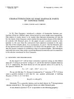
Corollary 2.2. If a graph G = (V, E) contains an odd wheel, then the encoding of 3-
colorability of G from Theorem 2.1 has a d egree one Nullstellensatz certificate of infeasi-
bility.
the electronic journal of combinatorics 17 (2010), #R114 6
n
3
5
7
8
9
10
11
2
4
6
1
Figure 2: Odd wheel

Proof. Assume G contains an odd wheel with vertices labelled as in Figure 2 below. Let
C := {(i, 1, i + 1) : 2  i  n −1}∪{(n, 1, 2)}.
Figure 2 illustrates the arc directions for the oriented partial 3-cycles of C. Each
edge of G is covered by exactly zero or two partial 3-cycles, so C satisfies Condition 1 of
Theorem 2.1. Furthermore, each a r c (1, i) ∈ Arcs(G) is covered exactly once by a partial
3-cycle in C, and there is an odd number of such arcs. Thus, C also satisfies Condition 2
of Theorem 2.1.
A non-trivial example of a non-3-colorable graph with a degree one Nullstellensatz
certicate is the Gr¨otzsch graph.
Example 2.3. Con s i der the Gr¨otzsch graph in Figure 3, which has no 3-cycles. T he
following set of oriented chordless 4-cycles gives a certificate of non-3-colorability by The-
orem 2.1:
C := {(1, 2, 3, 7), (2, 3, 4, 8), (3, 4, 5 , 9), (4, 5, 1, 10), (1, 10, 11, 7),
(2, 6, 11, 8), (3, 7, 11, 9), (4 , 8, 11, 10), (5, 9, 11, 6)}.
Figure 3 i ll ustrates the arc directions for the 4-cycles of C. Each edge of the graph is
covered by exactly two 4-cycles, so C satisfies C ondi tion 1 of Theorem 2.1. Moreover,
one can check that Condition 2 is also satisfied. It follows that the graph has no proper
3-coloring.
We now prove Theorem 2.1 using ideas from polynomial algebra. First, notice that
we can simplify a degree one certificate as follows: Expanding the left-hand side of (3)
and collecting terms, the only coefficient of x
j
x
3
i
is a
ij
and thus a
ij
= 0 for all i, j ∈ V .

Similarly, the only coefficient of x
i
x
j
is b
ij
, and so b
ij
= 0 for all {i, j} ∈ E. We thus
arrive at the fo llowing simplified expression:

i∈V
a
i
(x
3
i
+ 1) +

{i,j}∈E
(

k∈V
b
ijk
x
k
)(x
2
i

+ x
i
x
j
+ x
2
j
) = 1. (4)
the electronic journal of combinatorics 17 (2010), #R114 7
Figure 3 : Gr¨otzsch graph.
Now, consider the following set F of polynomials:
x
3
i
+ 1 ∀i ∈ V, (5)
x
k
(x
2
i
+ x
i
x
j
+ x
2
j
) ∀{i, j} ∈ E, k ∈ V. (6)
The elements of F are those polynomials that can appear in a degree one certificate
of infeasibility. Thus, there exists a degree one certificate if and only if the constant

polynomial 1 is in the linear span of F ; that is, 1 ∈ F
F
2
, where F 
F
2
is the vector space
over F
2
generated by the polynomials in F .
We next simplify the set F . Let H be the following set of polynomials:
x
2
i
x
j
+ x
i
x
2
j
+ 1 ∀{i, j} ∈ E,
(7)
x
i
x
2
j
+ x
j

x
2
k
∀(i, j), (j, k), (k, i) ∈ Arcs(G),
(8)
x
i
x
2
j
+ x
j
x
2
k
+ x
k
x
2
l
+ x
l
x
2
i
∀(i, j), (j, k), (k, l), (l, i) ∈ Arcs(G ) , (i, k), (j, l) ∈ Arcs(G).
(9)
If we identify the monomials x
i
x

2
j
as the a r cs (i, j), then the polynomials (8) correspond
to oriented partial 3-cycles and the polynomials (9) correspond to oriented chordless 4-
cycles. The following lemma says that we can use H instead of F to find a degree one
certificate.
Lemma 2.4. We have 1 ∈ F 
F
2
if and o nly if 1 ∈ H
F
2
.
Proof. The polynomials (6) above can be split into two classes of equations: (i) k = i or
k = j and (ii) k = i and k = j. Thus, the set F consists of
x
3
i
+ 1 ∀i ∈ V, (10)
x
i
(x
2
i
+ x
i
x
j
+ x
2

j
) = x
3
i
+ x
2
i
x
j
+ x
i
x
2
j
∀{i, j} ∈ E, (11)
x
k
(x
2
i
+ x
i
x
j
+ x
2
j
) = x
2
i

x
k
+ x
i
x
j
x
k
+ x
2
j
x
k
∀{i, j} ∈ E, k ∈ V, i = k = j. (12)
the electronic journal of combinatorics 17 (2010), #R114 8
Using polynomials (10) to eliminate the x
3
i
terms from (11), we arrive at the f ollowing set
of polynomials, which we label F
′
:
x
3
i
+ 1 ∀i ∈ V,
(13)
x
2
i

x
j
+ x
i
x
2
j
+ 1 = (x
3
i
+ x
2
i
x
j
+ x
i
x
2
j
) + (x
3
i
+ 1) ∀{i, j} ∈ E,
(14)
x
2
i
x
k

+ x
i
x
j
x
k
+ x
2
j
x
k
∀{i, j} ∈ E, k ∈ V, i = k = j.
(15)
Observe that F 
F
2
= F
′

F
2
. We can eliminate the polynomials (13) as follows. For
every i ∈ V , (x
3
i
+ 1) is the only polynomial in F
′
containing the monomial x
3
i

and
thus the polynomial (x
3
i
+ 1) cannot be present in any nonzero linear combination of the
polynomials in F
′
that equals 1. We arrive at the following smaller set of polynomials,
which we label F
′′
.
x
2
i
x
j
+ x
i
x
2
j
+ 1 ∀{i, j} ∈ E, (16)
x
2
i
x
k
+ x
i
x

j
x
k
+ x
2
j
x
k
∀{i, j} ∈ E, k ∈ V, i = k = j. (17)
So f ar, we have shown 1 ∈ F
F
2
= F
′

F
2
if and only if 1 ∈ F
′′

F
2
.
Next, we eliminate monomials of the fo rm x
i
x
j
x
k
. There are 3 cases to consider.

Case 1: {i, j} ∈ E but {i, k} ∈ E and {j, k} ∈ E. In this case, the monomial x
i
x
j
x
k
appea rs in only o ne polynomial, x
k
(x
2
i
+ x
i
x
j
+ x
2
j
) = x
2
i
x
k
+ x
i
x
j
x
k
+ x

2
j
x
k
, so we can
eliminate all such polynomials.
Case 2: i, j, k ∈ V , (i, j), (j, k), (k, i) ∈ Arcs(G). Graphically, this represents a 3-cycle
in the graph. In this case, the monomial x
i
x
j
x
k
appea rs in three polynomials:
x
k
(x
2
i
+ x
i
x
j
+ x
2
j
) = x
2
i
x

k
+ x
i
x
j
x
k
+ x
2
j
x
k
, (18)
x
j
(x
2
i
+ x
i
x
k
+ x
2
k
) = x
2
i
x
j

+ x
i
x
j
x
k
+ x
j
x
2
k
, (19)
x
i
(x
2
j
+ x
j
x
k
+ x
2
k
) = x
i
x
2
j
+ x

i
x
j
x
k
+ x
i
x
2
k
. (20)
Using the first polynomial, we can eliminate x
i
x
j
x
k
from the o t her two:
x
2
i
x
j
+ x
j
x
2
k
+ x
2

i
x
k
+ x
2
j
x
k
= (x
2
i
x
j
+ x
i
x
j
x
k
+ x
j
x
2
k
) + (x
2
i
x
k
+ x

i
x
j
x
k
+ x
2
j
x
k
),
x
i
x
2
j
+ x
i
x
2
k
+ x
2
i
x
k
+ x
2
j
x

k
= (x
i
x
2
j
+ x
i
x
j
x
k
+ x
i
x
2
k
) + (x
2
i
x
k
+ x
i
x
j
x
k
+ x
2

j
x
k
).
We can now eliminate the polynomial (18). Moreover, we can use the polynomials (16)
to rewrite the above two polynomials as follows.
x
k
x
2
i
+ x
i
x
2
j
= (x
2
i
x
j
+ x
j
x
2
k
+ x
2
i
x

k
+ x
2
j
x
k
) + (x
j
x
2
k
+ x
2
j
x
k
+ 1) + (x
i
x
2
j
+ x
2
i
x
j
+ 1),
x
i
x

2
j
+ x
j
x
2
k
= (x
i
x
2
j
+ x
i
x
2
k
+ x
2
i
x
k
+ x
2
j
x
k
) + (x
i
x

2
k
+ x
2
i
x
k
+ 1) + (x
j
x
2
k
+ x
2
j
x
k
+ 1).
Note that both of these polynomials correspond to two of the arcs of the 3-cycle (i, j),
(j, k), (k, i) ∈ Arcs(G) .
the electronic journal of combinatorics 17 (2010), #R114 9
Case 3: i, j, k ∈ V , (i, j), (j, k) ∈ Arcs(G ) and (k, i) ∈ Arcs(G). We have
x
k
(x
2
i
+ x
i
x

j
+ x
2
j
) = x
2
i
x
k
+ x
i
x
j
x
k
+ x
2
j
x
k
, (21)
x
i
(x
2
j
+ x
j
x
k

+ x
2
k
) = x
i
x
2
j
+ x
i
x
j
x
k
+ x
i
x
2
k
. (22)
As before we use the first polynomial to eliminate the monomial x
i
x
j
x
k
from the second:
x
i
x

2
j
+ x
j
x
2
k
+ (x
2
i
x
k
+ x
i
x
2
k
+ 1) = (x
i
x
2
j
+ x
i
x
j
x
k
+ x
i

x
2
k
) + (x
2
i
x
k
+ x
i
x
j
x
k
+ x
2
j
x
k
)
+ (x
j
x
2
k
+ x
2
j
x
k

+ 1).
We can now eliminate ( 21); thus, the original system has been reduced to the following
one, which we label as F
′′′
:
x
2
i
x
j
+ x
i
x
2
j
+ 1 ∀{i, j} ∈ E, (23)
x
i
x
2
j
+ x
j
x
2
k
∀(i, j), (i, k), (j, k) ∈ Arcs(G), (24)
x
i
x

2
j
+ x
j
x
2
k
+ (x
2
i
x
k
+ x
i
x
2
k
+ 1) ∀(i, j), (j, k) ∈ Arcs(G), (k, i) ∈ Arcs(G). (25)
Note that 1 ∈ F 
F
2
if and only if 1 ∈ F
′′′

F
2
.
The monomials x
2
i

x
k
and x
i
x
2
k
with (k, i) ∈ Arcs(G) always appear together and only
in t he polynomials (25) in the expression (x
2
i
x
k
+ x
i
x
2
k
+ 1). Thus, we can eliminate the
monomials x
2
i
x
k
and x
i
x
2
k
with (k, i) ∈ Arcs(G) by choosing one of the polynomials (25)

and using it to eliminate the expression (x
2
i
x
k
+ x
i
x
2
k
+ 1) from all other polynomials in
which it appears. Let i, j, k, l ∈ V be such that (i, j), (j, k), (k, l), (l, i) ∈ Arcs(G) and
(k, i), (i, k) ∈ Arcs(G). We can then eliminate the monomials x
2
i
x
k
and x
i
x
2
k
as follows:
x
i
x
2
j
+ x
j

x
2
k
+ x
k
x
2
l
+ x
l
x
2
i
= (x
i
x
2
j
+ x
j
x
2
k
+ x
2
i
x
k
+ x
i

x
2
k
+ 1)
+ (x
k
x
2
l
+ x
l
x
2
i
+ x
2
i
x
k
+ x
i
x
2
k
+ 1).
Finally, aft er eliminating the polynomials (25), we have system H (polynomials (7) , (8),
and (9)):
x
2
i

x
j
+ x
i
x
2
j
+ 1 ∀{i, j} ∈ E,
x
i
x
2
j
+ x
j
x
2
k
∀(i, j), (j, k), (k, i) ∈ Arcs(G),
x
i
x
2
j
+ x
j
x
2
k
+ x

k
x
2
l
+ x
l
x
2
i
∀(i, j), (j, k), (k, l), (l, i) ∈ Arcs(G ) , (i, k), (j, l) ∈ Arcs(G).
The system H has the pro perty that 1 ∈ F
′′′

F
2
if and only if 1 ∈ H
F
2
, and thus,
1 ∈ F 
F
2
if and only if 1 ∈ H
F
2
as required
We now establish that the sufficient condition for infeasibility 1 ∈ H
F
2
is equivalent

to the combinatorial parity conditions in Theorem 2.1.
Lemma 2.5. There exists a set C of oriented partial 3-cycles and oriented chordless
4-cycles satisfying Condi tion s 1. and 2. of Theorem 2.1 if and only if 1 ∈ H
F
2
.
the electronic journal of combinatorics 17 (2010), #R114 10
Proof. Assume that 1 ∈ H
F
2
. Then there exist coefficients c
h
∈ F
2
such that

h∈H
c
h
h =
1. Let H
′
:= {h ∈ H : c
h
= 1}; t hen,

h∈H
′
h = 1. Let C be the set of orient ed partial
3-cycles (i, j, k) where x

i
x
2
j
+x
j
x
2
k
∈ H
′
together with the set of oriented chordless 4-cycles
(i, j, l, k) where x
i
x
2
j
+ x
j
x
2
l
+ x
l
x
2
k
+ x
k
x

2
i
∈ H
′
. Now, |C
(i,j)
| is the number of polynomials
in H
′
of the form (8) or (9) in which the monomial x
i
x
2
j
appea rs, and similarly, |C
(j,i)
|
is the number of polynomials in H
′
of the f orm (8) or (9) in which the monomial x
j
x
2
i
appea rs. Thus,

h∈H
′
h = 1 implies that, for every pair x
i

x
2
j
and x
j
x
2
i
, either
1. |C
(i,j)
| ≡ 0 (mod 2), |C
(j,i)
| ≡ 0 (mod 2), and x
2
i
x
j
+ x
i
x
2
j
+ 1 ∈ H
′
or
2. |C
(i,j)
| ≡ 1 (mod 2), |C
(j,i)

| ≡ 1 (mod 2), and x
2
i
x
j
+ x
i
x
2
j
+ 1 ∈ H
′
.
In either case, we have |C
(i,j)
|+ |C
(j,i)
| ≡ 0 (mod 2). Moreover, since

h∈H
′
h = 1, there
must be an odd number of the polynomials of the form x
2
i
x
j
+ x
i
x

2
j
+ 1 in H
′
. That is,
case 2 above occurs an odd number of times and therefore,

(i,j)∈Arcs(G),i<j
|C
(i,j)
| ≡ 1
(mod 2) as required.
Conversely, assume that there exists a set C of oriented partial 3-cycles a nd oriented
chordless 4 -cycles satisfying the conditions o f Theorem 2.1. Let H
′
be the set of polyno-
mials x
i
x
2
j
+ x
j
x
2
k
where (i, j, k) ∈ C and the set of polynomials x
i
x
2

j
+ x
j
x
2
l
+ x
l
x
2
k
+ x
k
x
2
i
where (i, j, l, k) ∈ C together with the set of polynomials x
2
i
x
j
+ x
i
x
2
j
+ 1 ∈ H where
|C
(i,j)
| ≡ 1. Then, |C

(i,j)
| + |C
(j,i)
| ≡ 0 (mod 2) implies that every monomial x
i
x
2
j
ap-
pear s in an even number polynomials of H
′
. Moreover, since

(i,j)∈Arcs(G),i<j
|C
(i,j)
| ≡ 1
(mod 2), there are an odd number of polynomials x
2
i
x
j
+x
i
x
2
j
+1 appearing in H
′
. Hence,


h∈H
′
h = 1 and 1 ∈ H
F
2
.
Combining Lemmas 2.4 and 2.5, we arrive at the characterization stated in Theo-
rem 2.1. That such graphs can be decided in polynomial time follows from the fact that
the existence of a certificate of any fixed degree can be decided in polynomial time (as
is well known and follows since there are polynomially many monomials up to any fixed
degree; see also [34, Theorem 4.1.3]).
Finally, we pose as open problems the construction of a variant of Theorem 2.1 for
general k-colorability and also combinatorial characterizations for larger certificate degrees
D.
Problem 2.6. Characterize those graphs with a given k-colorability Nullstellensatz cer-
tificate of degree D.
3 Recognizin g Uniquely Hamiltonian Graphs
Throughout this section we work over an arbitrary algebraically closed field K = K,
although in some cases, we will need to restrict its characteristic. Let us denote by H
G
the Hamiltonian ideal generated by the polynomials from Proposition 1.3. A connected,
directed graph G with n vertices has a Hamiltonian cycle if and only if the equations
defined by H
G
have a solution over K (or, in other words, if a nd only if V (H
G
) = ∅ for
the electronic journal of combinatorics 17 (2010), #R114 11
the algebraic variety V (H

G
) associated to the ideal H
G
). In a precise sense to be made
clear below, the ideal H
G
actually encodes all Hamiltonian cycles of G. However, we need
to be somewhat careful about how to count cycles (see Lemma 3.8). In practice ω can be
treated as a variable and not as a fixed primitive n-th root of unity. A set of equations
ensuring that ω only takes on the value of a primitive n-th root of unity is t he following:
{ω
i(n−1)
+ ω
i(n−2)
+ ···+ ω
i
+ 1 = 0 : 1  i  n}.
We can also use the cyclotomic polynomial Φ
n
(ω) [16], which is the polynomial whose
zeroes are the primitive n-th roots of unity.
We shall utilize the theory of Gr¨obner bases to show that H
G
has a special (alge-
braic) decomposition structure in terms of the different Hamiltonian cycles of G (this is
Theorem 3.9 below). In the particular case when G has a unique Hamiltonian cycle, we
get a sp ecific algebraic criterion which can be algorithmically verified. These results are
Hamiltonian analogues to the algebraic k-colorability characterizations of [24]. We first
turn our attention more generally to cycle ideals of a simple directed graph G. These
will be the basic elements in our decomposition of the Hamiltonian ideal H

G
, as they
algebraically encode single cycles C (up to symmetry).
When G has the property that each pair of vertices connected by an arc is also con-
nected by an arc in the opposite direction, then we call G doubly covered. When G = (V, E)
is presented as an undirected graph, we shall always view it as the doubly covered directed
graph on vertices V with arcs Arcs(G).
Let C be a cycle of length k > 2 in G, expressed as a sequence o f arcs,
C = {(v
1
, v
2
), (v
2
, v
3
), . . . , (v
k
, v
1
)}.
For the purpose of this work, we call C a doubly cove red cycle if consecutive vertices
in the cycle are connected by ar cs in both directions; otherwise, C is simply called di-
rected. In par ticular, each cycle in a doubly covered graph is a doubly covered cycle.
These definitions allow us to work with both undirected and directed g r aphs in the same
framework.
Definition 3.1 (Cycle encodings). Let ω be a fixed primitive k-th root of unity and let
K be a fi e l d with c haracteristic not d i viding k. If C is a doubly cov ered cycle of len gth k
and the vertices i n C a re {v
1

, . . . , v
k
}, then the cycle encoding of C is the following set of
k polynomials in K[x
v
1
, . . . , x
v
k
]:
g
i
=





x
v
i
+
(ω
2+i
−ω
2−i
)
(ω
3
−ω)

x
v
k−1
+
(ω
1−i
−ω
3+i
)
(ω
3
−ω)
x
v
k
i = 1 , . . . , k − 2,
(x
v
k−1
− ωx
v
k
)(x
v
k−1
− ω
−1
x
v
k

) i = k − 1,
x
k
v
k
−1 i = k.
(26)
If C is a directed cycle of length k in a directed graph, with vertex set {v
1
, . . . , v
k
}, the
cycle encoding of C is the following set of k polynomials:
g
i
=

x
v
k−i
−ω
k−i
x
v
k
i = 1, . . . , k − 1,
x
k
v
k

− 1 i = k.
(27)
the electronic journal of combinatorics 17 (2010), #R114 12
Definition 3.2 (Cycle Ideals). Th e cycle ideal associated to a cycle C is
H
G,C
= g
1
, . . . , g
k
 ⊆ K[x
v
1
, . . . , x
v
k
],
where the g
i
s are the cycle encoding of C giv en by (26) or (27).
The polynomials g
i
are computationally useful generators for cycle ideals. (Once again,
see [11] for the relevant background on Gr¨obner bases and term orders.)
Lemma 3.3. The se t of cycle encoding polynomials F = {g
1
, . . . , g
k
} is a reduced Gr¨obner
basis for the cycle ideal H

G,C
with respect to any term order ≺ with x
v
k
≺ ··· ≺ x
v
1
.
Proof. Since the leading monomials in a cycle encoding:
{x
v
1
, . . . , x
v
k−2
, x
2
v
k−1
, x
k
v
k
} or {x
v
1
, . . . , x
v
k−2
, x

v
k−1
, x
k
v
k
} (28)
are relatively prime, the polynomials g
i
form a Gr¨obner basis for H
G,C
(see Theorem 3
and Proposition 4 in [11, Section 2]). That F is reduced follows from inspection of (26)
and (27).
Remark 3.4. In particular, since reduced Gr¨obner bases (with respect to a fixed term
order) are unique, it follows that cycle encodings are canonical w ays of generating cycle
ideals (and thus of representing cycles by Lemma 3.6).
Having explicit Gr¨obner bases for these ideals allows us to compute their Hilbert series
easily.
Corollary 3.5. The Hilbert series of K[x
v
1
, . . . , x
v
k
]/H
G,C
for a doubly covered cycle or
a directed cycle is equal to (respectively)
(1 −t

2
)(1 −t
k
)
(1 − t)
2
or
(1 −t
k
)
(1 − t)
.
Proof. If ≺ is a graded term order, then the (affine) Hilbert function of an ideal and o f
its ideal of leading terms are the same [1 1, Chapter 9, §3]. The form of the Hilbert series
is now immediate from (28).
The naming of these ideals is motivated by the following result; in words, it says t hat
the cycle C is encoded as a complete intersection by the ideal H
G,C
.
Lemma 3.6. The following hold for the ideal H
G,C
.
1. H
G,C
is radical,
2. |V (H
G,C
)| = k if C is directed, and |V (H
G,C
)| = 2k if C is doubly covered undirected.

the electronic journal of combinatorics 17 (2010), #R114 13
Proof. Without loss of generality, we suppose that v
i
= i for i = 1, . . . , k. Let ≺ be any
term order in which x
k
≺ ··· ≺ x
1
. From Lemma 3.3, the set of g
i
form a Gr¨obner basis
for H
G,C
. It follows that the number of standard monomials of H
G,C
is 2k if C is doubly
covered undirected (resp. k if it is directed). Therefore by [24, Lemma 2.1], if we can
prove that |V (H
G,C
)|  k (resp. |V (H
G,C
)|  2k), then both statements 1. and 2. follow.
When C is directed, t his follows easily from t he form of (27), so we shall assume that C
is doubly covered undirected. We claim that the k cyclic permutations of the two points:
(ω, ω
2
, . . . , ω
k
), (ω
k

, ω
k−1
, . . . , ω)
are zeroes of g
i
, i = 1, . . . , k. Since cyclic permutation is multiplication by a power of ω,
it is clear that we need only verify this claim for the two points above. In the fist case,
when x
i
= ω
i
, we compute that for i = 1, . . . , k − 2:
(ω
3
− ω)g
i
(ω, . . . , ω
k
) = (ω
3
−ω)ω
i
+ (ω
2+i
− ω
2−i
)ω
k−1
+ (ω
1−i

− ω
3+i
)ω
k
= ω
3+i
−ω
1+i
+ ω
1+i+k
− ω
1−i+k
+ ω
1−i+k
− ω
3+i+k
= 0,
since ω
k
= 1. In the second case, when x
i
= ω
1−i
, we again compute that for i =
1, . . . , k − 2:
(ω
3
− ω)g
i
(ω

k
, . . . , ω) = (ω
3
−ω)ω
1−i
+ (ω
2+i
− ω
2−i
)ω
2
+ (ω
1−i
− ω
3+i
)ω
= ω
4−i
−ω
2−i
+ ω
4+i
− ω
4−i
+ ω
2−i
− ω
4+i
= 0.
Finally, it is obvious that the two points zero g

k−1
and g
k
, and this completes the proof.
Remark 3.7. Conversely, it is eas y to see that points in V (H
G,C
) correspond to cycles
of length k in G. That this variety contains k or 2k points corresponds to there being k
or 2k ways of writing dow n the cycle since we ma y cyclically permute it and also reverse
its orientation (if each arc in the path is bidirectional).
Before stating our decomposition theorem (Theorem 3.9), we need to explain how the
Hamiltonian ideal enco des all Hamiltonian cycles o f the graph G.
Lemma 3.8. Let G be a connected directed graph on n vertices. Then,
V (H
G
) =

C
V (H
G,C
),
where the union is over all Hamiltonian c ycle s C in G.
Proof. We only need to verify that points in V (H
G
) correspond to cycles of length n.
Suppose there exists a Hamiltonian cycle in the graph G. Label ver t ex 1 in the cycle with
the number x
1
= ω
0

= 1 and then successively label vertices along the cycle with one
the electronic journal of combinatorics 17 (2010), #R114 14
higher power of ω. It is clear that these la bels x
i
associated to vertices i zero all of the
equations generating H
G
.
Conversely, let v = (x
1
, . . . , x
n
) be a point in the variety V (H
G
) associated t o H
G
; we
claim that v encodes a Hamiltonian cycle. From the edge equations, each vertex must be
adjacent to one labeled with the next highest power of ω. Fixing a starting vertex i, it
follows that there is a cycle C labeled with (consecutively) increasing powers of ω. Since ω
is a primitive nth root of unity, this cycle must have length n, and thus is Hamiltonian.
Combining all of these ideas, we can prove the following result.
Theorem 3.9. Let G be a connected directed graph with n vertices. Then,
H
G
=

C
H
G,C

,
where C ranges over all Hamiltonian cycles of the graph G.
Proof. Since H
G
contains a square-free univariate polynomial in each indeterminate, it is
radical (see f or instance [24, Lemma 2 .1 ]). It follows that
H
G
= I(V (H
G
))
= I


C
V (H
G,C
)

=

C
I(V (H
G,C
))
=

C
H
G,C

,
(29)
where t he second inequality comes from Lemma 3.8 and the last one from H
G,C
being a
radical ideal (Lemma 3.6).
We call a directed graph (resp. doubly covered graph) un i quely Hamiltonian if it
contains n cycles of length n (resp. 2 n cycles of length n).
Corollary 3.10. The graph G is uniq uely Hamiltonia n if and only if the Hamiltonian
ideal H
G
is of the form H
G,C
for some length n cycle C.
This corollary provides an algorithm to check whether a graph is uniquely Hamiltonian.
We simply compute a unique reduced Gr¨obner basis of H
G
and then check that it has
the same form as that of an ideal H
G,C
. Another approach is to count the number of
standard monomials of any Gr¨obner bases for H
G
and compare with n or 2n (since H
G
is
radical). We remark, however, that it is well-known that computing a Gr¨obner basis in
general cannot be done in polynomial time [51, p. 400].
We close this section with a directed and an undirected example of Theorem 3 .9.
the electronic journal of combinatorics 17 (2010), #R114 15

Example 3.11. Let G be the directed graph with vertex set V = {1, 2, 3, 4, 5} and arcs
A = {(1, 2), (2, 3), (3, 4), (4, 5), (5, 1), (1 , 3), (1, 4)}. Moreover, let ω be a primitive 5-th root
of unity. The ideal H
G
⊂ K[x
1
, x
2
, x
3
, x
4
, x
5
] is generated by the polynomials, {x
5
i
− 1 :
1  i  5} union with the polynomials
{(ωx
1
− x
2
)(ωx
1
−x
3
)(ωx
1
−x

4
), ωx
2
− x
3
, ωx
3
− x
4
, ωx
4
− x
5
, ωx
5
−x
1
}.
A reduced Gr¨obner basis for H
G
with respect to the ordering x
5
≺ x
4
≺ x
3
≺ x
2
≺ x
1

is
{x
5
5
−1, x
4
−ω
4
x
5
, x
3
−ω
3
x
5
, x
2
−ω
2
x
5
, x
1
−ωx
5
},
which is a generating set for H
G,C
with C = {(1 , 2), (2, 3), ( 3 , 4), (4, 5 ), (5, 1)}.

Let G be an undirected graph with vertex set V and edge set E, and consider the
auxiliary directed graph
˜
G with vertices V and ar cs Arcs(G). Notice t hat
˜
G is doubly
covered, and hence each of its cycles are doubly covered. We apply Theorem 3.9 to H
˜
G
to
determine and count Hamiltonian cycles in G. In particular, the cycle C = {v
1
, v
2
, . . . , v
n
}
of G is Hamiltonian if a nd only if the two cycles
{(v
1
, v
2
), (v
2
, v
3
), . . . , (v
n−1
, v
n

), (v
n
, v
1
)}, {(v
2
, v
1
), (v
3
, v
2
), . . . , (v
n
, v
n−1
), (v
1
, v
n
)}
are Hamiltonian cycles of
˜
G.
Example 3.12. Let G be the undi rected comple te graph on the vertex set V = {1, 2, 3, 4}.
Let
˜
G be the doubly covered graph with vertex set V and arcs Arcs(G). Notice that
˜
G has

twelve Hamilton i an cycles:
C
1
={(1, 2), (2, 3), (3, 4), (4, 1)}, C
2
={(2, 1), (3, 2), (4, 3), (1, 4)},
C
3
={(1, 2), (2, 4), (4, 3), (3, 1)}, C
4
={(2, 1), (4, 2), (3, 4), (1, 3)},
C
5
={(1, 3), (3, 2), (2, 4), (4, 1)}, C
6
={(3, 1), (2, 3), (4, 2), (1, 4)},
C
7
={(1, 3), (3, 4), (4, 2), (2, 1)}, C
8
={(3, 1), (4, 3), (2, 4), (1, 2)},
C
9
={(1, 4), (4, 2), (2, 3), (3, 1)}, C
10
={(4, 1), (2, 4), (3, 2), (1, 3)},
C
11
={(1, 4), (4, 3), (3, 2), (2, 1)}, C
12

={(4, 1), (3, 4), (2, 3), (1, 2)}.
One can check in a symbolic algebra system s uch as SINGULAR or Macaulay 2 th at the
ideal H
˜
G
is the intersection of the cycle ideals H
˜
G,C
i
for i = 1 , . . . , 12.
4 Permutation Groups as Algebraic Varieties and
their Convex App roximations
In this section, we study convex hulls of permutations groups viewed as permutation
matrices. We begin by studying the convex hull of automorphism groups of undirected
simple graphs; these have a natural polynomial presentation using Proposition 1.4 from
the introduction. For background material on graph automorphism groups see [7, 8].
the electronic journal of combinatorics 17 (2010), #R114 16
We write Aut(G) for the automorphism group of a graph G = (V, E). Elements of
Aut(G) are naturally represented as |V |×|V | permutation matrices; they are the integer
vertices of the rational polytope P
G
defined in the discussion following Proposition 1.4.
The polytope P
G
was first introduced by Tinhofer [48]. Since we are primarily interested
in the integer vertices of P
G
, we investigate IP
G
, the integer hull of P

G
(i.e. IP
G
=
conv(P
G
∩ Z
n×n
)). In the fortunate case that P
G
is already integral (P
G
= IP
G
), we say
that the graph G is compac t, a term coined in [48]. This occurs, for example, in the
special case that G is an independent set on n vertices. In this case Aut(G) = S
n
and
P
G
is the well-studied Birkhoff po lytope, the convex hull of all doubly-stochastic matrices
(see Chapter 5 of [27]). One can therefore view P
G
as a generalization of the Birkhoff
polytope to arbitrary graphs. Unfor t unately, the polytope P
G
is not always integral. Fo r
instance, P
G

is not integral when G is the Petersen graph. Nevertheless, we can prove the
following related result.
Proposition 4.1. The polytope P
G
is quasi-integral. That is, the induced subgraph of the
integer points of the 1-skeleton of P
G
is connected.
Proof. We claim that there exists a 0/1 matrix A such that P
G
is the set of points
{x ∈ R
n×n
: Ax = 1, x  0} (where 1 is the all 1s vector). By the main theorem
of Trubin [49] and independently [4], polytopes given by such systems ar e quasi-integral
(see also Theorem 7.2 in Chapter 4 of [27]). Therefore, we need to r ewrite the defining
equations presented in Proposition 1.4 to fit this desired shape. Fix indices 1  i, j  n
and consider the row of P
G
defined by the equation

r∈δ(j)
P
ir
−

k∈δ(i)
P
kj
= 0.

Here δ(i) denotes those vertices j which are connected to i. Adding

n
r=1
P
rj
= 1 to bo t h
sides of t his expression yields

r∈δ(j)
P
ir
+

k /∈δ(i)
P
kj
= 1. (30)
We can therefore replace the original n
2
equations defining P
G
by (30) over all 1 
i, j  n. The result now follows provided that no summand in each of these equations
repeats. However, this is clear since if summands P
kj
and P
ir
are the same, then r = j,
which is impossible since r ∈ δ(j).

We would still like to find a tighter description of IP
G
in terms of inequalities. For
this purpose, recall the radical polynomial ideal I
G
in Proposition 1.4 and its real variety
V
R
(I
G
). We approximate a tighter description of IP
G
using a hierarchy of projected
semidefinite relaxations of conv(V
R
(I
G
)). When these relaxations are tight, we obtain a
full description of IP
G
that allows us to optimize and determine feasibility via semidefinite
programming.
We begin with some preliminary definitions from [21] and motivated by Lov´asz &
Schrijver [33]. Let I ⊂ R[x
1
, . . . , x
n
] be a real radical ideal (I = I(V
R
(I))). A polynomial

the electronic journal of combinatorics 17 (2010), #R114 17
f is said to be nonnegative mod I (written f  0 (mod I)) if f (p)  0 for all p ∈ V
R
(I).
Similarly, a polynomial f is said to be a sum of squares mod I if there exist h
1
, . . . , h
m
∈
R[x
1
, . . . , x
n
] such that f −

m
i=1
h
2
i
∈ I. If the degrees of the h
1
, . . . , h
m
are bounded by
some positive integer k, we say f is k-sos mod I.
The k-th theta body o f I, denoted T H
k
(I), is the subset of R
n

that is nonnegative
on each f ∈ I that is k-sos mod I. We say that a real variety V
R
(I) is theta k-exact if
conv(V
R
(I)) = T H
k
(I). When the ideal I is real radical, theta bodies provide a hierarchy
of semidefinite relaxations of conv(V
R
(I)):
T H
1
(I) ⊇ T H
2
(I) ⊇ ··· ⊇ conv(V
R
(I))
because in this case theta bodies can be expressed as projections of feasible regions of
semidefinite prog r ams (such regions are called spectrahedra). In order to exploit this
theory, we must establish that I
G
is indeed real radical.
Lemma 4.2. The ideal I
G
⊆ R[x
1
, . . . , x
n

] is real radical.
Proof. Let J
G
be the ideal in C[x
1
, . . . , x
n
] generated by the same polynomials that gen-
erate I
G
, and
R
√
I
G
be the real radical of I
G
. Since the polynomial x
2
i
− x
i
∈ J
G
for each
1  i  n, Lemma 2.1 of [24] implies J
G
=
√
J

G
(where
√
J
G
is the radical of J
G
). Together
with the fact that V
C
(J
G
) = V
R
(I
G
), this implies J
G
⊇
R
√
I
G
. Since I
G
= J
G
∩R[x
1
, . . . , x

n
],
we conclude I
G
⊇
R
√
I
G
. The result follows since trivially, I
G
⊆
R
√
I
G
.
From Lemma 4.2, we conclude that if I
G
is theta k-exact, linear optimization over the
automorphisms can be performed using semidefinite programming provided that one first
computes a basis for the quotient ring R[P
11
, P
12
, . . . , P
nn
]/I
G
(e.g., obtained from the

standard monomials of a Gr¨obner basis). Using such a basis one can set up the necessary
semidefinite programs (see Section 2 of [21] for details). In fact, for k-exact ideals, one
only needs those elements of the basis up to degree 2k. This motivates the need for
characterizing those graphs for which I
G
is k-exact.
In this section we focus on finding graphs G such that I
G
is 1-exact; we shall call
such graphs exact in what follows. The key to finding exact g raphs is the following
combinatorial-geometric characterization.
Theorem 4.3. [21] Let V
R
(I) ⊂ R
n
be a finite real varie ty. Then V
R
(I) is exact if and
only if there is a finite linear inequality description of conv(V
R
(I)) such that for every
inequality g(x)  0, there is a hyperplane g(x) = α such that every point in V
R
(I) l i es
either on the hyperplane g(x) = 0 or the hyperplane g(x) = α.
A result of Sullivant (see Theorem 2.4 in [46]) directly implies that when the polytope
P = conv(V
R
(I)) is lattice isomorphic to an integral polytope of the form [0, 1]
n

∩L where
L is an affine subspace, then P satisfies the condition of Theorem 4.3. Putting these ideas
together we can prove compactness implies exactness. Furthermore, the class of exact
graphs properly extends the class of compact graphs. The proof of this latter fact is an
extension of a result in [48 ].
the electronic journal of combinatorics 17 (2010), #R114 18
Theorem 4.4. The class of exact graphs strictly contains the clas s of compact graphs.
More precisely:
1. If G i s a compact graph, then G is also exact.
2. Let G
1
, . . . , G
m
be k-regular conn ected compact graphs, and let G =

m
i=1
G
i
be the
graph that is the disjoi nt union of G
1
, . . . , G
m
. Then G is always exact, but G may
not be compact. Indeed, G is compact if and only if G
i
∼
=
G

j
for all 1  i, j  n.
Proof. If G is compact, then the integer hull of P
G
is precisely the affine space
{P ∈ R
n×n
: P A
G
= A
G
P,
n

i=1
P
ij
=
n

j=1
P
ij
= 1, 1  i, j  n}
intersected with the cube [0, 1]
n×n
. That G is exact follows f r om Theorem 2.4 of [46].
We now prove Stat ement 2. If G
i


∼
=
G
j
for some pair (i, j), t hen G wa s shown to be
non-compact by Tinhofer (see [48, Lemma 2]). Nevertheless, G is exact. We prove this
for m = 2, and the result will follow by induction. We claim that if G = G
1
⊔ G
2
with
G
1

∼
=
G
2
, then the integer hull IP
G
is the solution set to the following system (which we
denote by
˜
IP
G
):
(P A
G
− A
G

P )
i,j
= 0 1  i, j  n,
n

i=1
P
i,j
= 1 1  j  n,
n

j=1
P
i,j
= 1 1  i  n,
n
1

i=1
n
1
+n
2

j=n
1
+1
P
i,j
= 0,

0  P
i,j
 1,
where n
i
= |V (G
i
)| with n
1
 n
2
. Statement 2 then follows again from Theorem 2.4 of
[46].
We now prove the claim. Let A
G
i
be t he adjacency matrix of G
i
. Index the adjacency
matrix of G = G
1
⊔ G
2
so that the first n
1
rows (and hence first n
1
columns) index the
vertices of G
1

. Any feasible P of P
G
can be written as a block matrix
P =

A
P
B
P
C
P
D
P

,
in which A
P
is n
1
×n
1
. Since G
1
and G
2
are not isomorphic, the only integer vertices of
P
G
are of the form


P
1
0
0 P
2

where P
i
is an automorphism of G
i
.
the electronic journal of combinatorics 17 (2010), #R114 19
Now let P be any non-integer vertex of P
G
. We claim that the row sums of B
P
must
be 1. This will establish that IP
G
is described by the system
˜
IP
G
. To see this, observe
that if Q is any point in P
G
not in IP
G
, it is a convex combination of points in P
G

, one
of which (say P ) is non-integer. If the row sums of B
P
are 1, then Q violates the system
˜
IP
G
.
We now prove t hat if P is a non-integer vertex of P
G
, then the row sums of B
P
must
be 1. Since P commutes with the adjacency matrix A
G
of G, we must have
A
P
A
G
1
= A
G
1
A
P
, B
P
A
G

2
= A
G
1
B
P
, C
P
A
G
2
= A
G
1
C
P
, D
P
A
G
2
= A
G
2
D
P
.
Let {b
1
, . . . , b

n
2
} be the column sums of B
P
. We shall calculate the sum of the entries
in each column of B
P
A
G
2
= A
G
1
B
P
in two ways. First, consider A
G
1
B
P
. Since G
1
is
k-regular, each entry of the i-th column of B
P
will contribute exactly k times to the sum
of the entries of the i-th column o f A
G
1
B

P
. Thus, the sum of the entries of the i-th column
of A
G
1
B
P
is kb
i
.
Second, consider B
P
A
G
2
. The sum of the entries in its i-t h column is the sum of the
entries o f t he columns of B
P
indexed by the neighbors of i in G
2
. Thus, the sum of the
entries in the i-th column of B
P
A
G
2
is

l∈δ
G

2
(i)
b
l
. It follows that kb
i
=

l∈δ
G
2
(i)
b
l
for
each 1  i  n. This equality can be written concisely as:

kI
n
2
×n
2
−A
G
2




b

1
.
.
.
b
n
2



= 0.
The matrix kI
n
2
×n
2
− A
G
2
is the Laplacian of G
2
. It is well known that the kernel of
the Laplacian of a connected graph is one dimensional (see [8], Lemma 13.1.1 ). Since G
2
is regular, the kernel contains the all ones vector. It follows that b
1
= ··· = b
n
2
. By a

similar argument, the row sums of C
P
are all the same. Since all row sums and column
sums of P are 1, and the row sums and column sums of A
G
1
are the same, it follows that
the row sums of B
P
are equal and are the same as the column sums of C
P
.
Now assume fo r contradiction that the row sums of B
P
are not 1. If the row sums are
0, t hen B
P
and C
P
would be 0 matrices. Since G
1
and G
2
are compact this would imply
A
P
and D
P
are permutation matrices, contradicting that P is not integral. Thus the sum
of each row of B

P
is λ with 0 < λ < 1. This implies the sum of the rows of A
P
is 1 − λ
and that
1
1−λ
A
P
is a feasible solution to P
G
1
. By compactness of G
1
, the matrix
1
1−λ
A
P
is a convex combination

k
i=1
µ
k
Q
k
of permutations Q
k
of G

1
. This implies that
P =
k

i=1
µ
i

(1 −λ)Q
k
B
P
C
P
D
P

,
which is a convex combination of feasible solutions to P
G
, contradicting P being a vertex.
It follows that the row sums of B
P
must be 1.
Exact graphs are then more abundant than compact graphs and the convex hull of
automorphisms of an exact graph has a description in terms of semidefinite programming.
the electronic journal of combinatorics 17 (2010), #R114 20
It is thus desirable to find nice classes o f graphs that are exact. Notice that exactness is
really a property of the set of permutation matrices representing an automorphism group.

This discussion motivates the following question.
Question 4.5. Which permutation subgroups of S
n
are exac t?
Here we view a permutation subgroup of S
n
through its natural permutation represen-
tation in R
n×n
. In this light, a permutation subgroup can be co nsidered as a variety, and
we say the permutation subgroup is exact if this variety is exact. As an example, consider
the alternating group A
n
as a subgroup of S
n
. It is known (see [7]) that A
n
is never the
automorphism group of a graph on n vertices, so it cannot be presented as the integer
points of a polytope of the form P
G
with |V (G)| = n. However, there is a description of
A
n
as a variety whose points are ver tices of the n ×n Birkhoff polytope:
n

j=1
P
i,j

= 1, 1  i  n;
n

i=1
P
i,j
= 1, 1  j  n;
det(P ) = 1; P
2
i,j
− P
i,j
= 0, 1  i, j  n.
More generally, when a finite permutation group has a description as a variety, we
can apply the theory of theta bo dies to obtain descriptions of convex hulls. Using t he
algebraic-geometric ideas outlined in [45] we give a sufficient condition for exactness of
permutation gro ups.
Let A = {σ
1
, . . . , σ
d
} be a subgroup of S
n
. We consider A as the set of matrices
{P
σ
1
, . . . , P
σ
d

} ⊆ Z
n×n
, where P
σ
i
is the permutation matrix corresp onding to σ
i
. Let
C[x] := C[x
σ
1
, . . . , x
σ
d
] be the polynomial ring in d indeterminates indexed by permuta-
tions in A, and let C[t] := C[t
ij
: 1  i, j  n].
The algebra homomorphism induced by the map
π : C[x] → C[t], π(x
σ
i
) =

1j,kn
t
(P
σ
i
)

jk
jk
(31)
has kernel I
A
, which is a prime toric ideal [45]. By Theorem 4.3, Corollary 8.9 in [45], and
Corollary 2.5 in [46], the group A is exact if and only if for every reverse lexicographic
term ordering ≺ on C[x], the initial ideal in
≺
(I
A
) is generated by square-free monomials.
We now describe a family of permutation groups that are exact.
Let A ⊆ Z
n×n
be a subgroup of S
n
. We say that A is permutation summable if for any
permutations P
1
, . . . , P
m
∈ A satisfying the inequality

m
i=1
P
i
− I  0 (entry-wise), we
have that


m
i=1
P
i
−I is also a sum of permutation matrices in A. For example, Birkhoff’s
Theorem (see e.g., Theorem 1.1 in Chapter 5 o f [27]) implies S
n
is permutation summable.
Note that in this case P
S
n
is the Birkhoff polytope which is known to be exact by the
results in [21]. We prove the following result.
Theorem 4.6. Let A = {σ
1
, . . . , σ
d
} be a permutation group that is a subgroup of S
n
.
(1) If A is permutation summable, then A is exa c t.
(2) Suppose I
A
, the toric ideal associated to A, has a quadratically generated Gr¨obner
basis with respect to any reverse lexicographic ordering ≺, then A i s exact.
the electronic journal of combinatorics 17 (2010), #R114 21
Proof. Let I
A
be the kernel of the algebra homomorphism induced by (31). We shall

abbreviate the action o f π on x
σ
by π(x
σ
) = t
P
σ
for any σ ∈ A.
Let G be a reduced Gr¨obner basis for I
A
with respect to some reverse lexicographic
order ≺ on {x
σ
1
, . . . , x
σ
d
}. Let x
u
− x
v
∈ G with leading term x
u
. By Theorem 4.3,
Corollary 8.9 in [45] and Corollary 2.5 in [46], Statement (1) follows if we can find a
square-free monomial x
u
′
∈ in
≺

(I
A
) such that x
u
′
divides x
u
.
Let x
τ
be the smallest variable dividing x
v
with respect to ≺. Then x
τ
is smaller
than any variable appearing in x
u
by the choice of a reverse lexicographic ordering. Since
x
u
− x
v
∈ G, we have π(x
u
) = π(x
v
). It follows that π(x
τ
) divides π(x
u

), so letting
x
u
= x
σ
i
1
···x
σ
i
k
for some {σ
i
1
, . . . , σ
i
k
} ⊆ A, we have
π(x
u
)
π(x
τ
)
= t
P
σ
i
1
+···+P

σ
i
k
t
−P
τ
,
in which

k
j=1
P
σ
i
j
− P
τ
is a matrix with nonnegative integer entries. Choose a subset
{ρ
1
, . . . , ρ
r
} ⊂ {σ
i
1
, . . . , σ
i
k
} such that {P
ρ

1
, . . . , P
ρ
r
} minimally supports P
τ
with P
ρ
i
=
P
ρ
j
for all i, j, and let x
u
′
= x
ρ
1
···x
ρ
r
. We claim that x
u
′
is a square-free monomial that
divides x
u
and lies in in
≺

(I
A
), which will prove Statement (1).
By construction, all indeterminates x
ρ
1
, . . . , x
ρ
r
are distinct, so x
u
′
is square-free.
Moreover, since {ρ
1
, . . . , ρ
r
} ⊂ {σ
i
1
, . . . , σ
i
k
}, we have that x
u
′
divides x
u
. It remains
to show that x

u
′
lies in in
≺
(I
A
). To see this, note that

r
i=1
P
ρ
i
− P
τ
has nonnegative
integer ent r ies, and hence so does
M =
r

i=1
(P
τ
)
−1
P
ρ
i
− I
(multiplying by P

−1
τ
permutes matrix entries, and t herefore does not effect nonnegativity).
Since A is permutation summable, the matrix M is a sum of matrices in A, and hence so
is P
τ
M =

r
i=1
P
ρ
i
−P
τ
. It follows that
r

i=1
P
ρ
i
− P
τ
=
r−1

j=1
P
σ

l
j
for some {σ
l
1
, . . . , σ
l
r −1
} ⊂ A. In particular, π(x
u
′
) = π(x
τ
)·π(x
v
′
) and so x
u
′
−x
τ
x
v
′
∈ I
A
.
Since x
τ
is smaller than any term in x

u
′
(the monomial x
u
′
divides x
u
and the same holds
for x
u
), the leading term of x
u
′
−x
τ
x
v
′
is x
u
′
; hence, x
u
′
∈ in
≺
(I
A
). This proves Statement
(1).

For Statement (2), since any Gr¨obner basis is quadratically generated, by part (1)
it suffices to show that if P
1
, P
2
, Q ∈ A with all entries o f P
1
+ P
2
− Q nonnegative,
then P
1
+ P
2
− Q is a permutation matrix. Since supp(Q) ⊂ supp(P
1
) ∪ supp( P
2
), the
permutation Q is a vertex of a face containing P
1
and P
2
. By Theorem 3.5 of [22], Q is on
the smallest face containing P
1
and P
2
, and this face is centr ally symmetric. Thus, there
is a vertex R such that Q + R = P

1
+ P
2
, and the result follows.
the electronic journal of combinatorics 17 (2010), #R114 22
In light of Theorem 4.6, we would like to find permutation groups A that are per-
mutation summable. As we have seen, Birkhoff’s Theorem (see [45]) implies that S
n
is
permutation summable. We can use this fact to constr uct more permutation summable
groups. For instance, S
n
1
× ··· × S
n
m
is permutation summable, simply by applying the
permutation summability condition on each S
n
i
and taking direct sums. More generally,
if H
1
, . . . , H
m
are permutation summable, then so is H
1
×···× H
m
. We present another

class of permutation summable groups that conta ins familiar groups.
Definition 4.7. Let A be a permutation subgroup of S
n
. We say A is strongly fixed-point
free if for every σ ∈ A\{1}, we have σ(i) = i for any i ∈ {1, . . . , n}.
Corollary 4.8. Let A be a strongly fixed-point free subgroup of S
n
. Then A is exact.
Proof. Let A be strongly fixed-point free. Consider any subset {P
σ
1
, . . . , P
σ
k
} of A and
assume

k
i=1
P
σ
i
−I is a matrix with nonnegative entries. Then one of the matrices in A
contains a fixed point. Without loss of generality, assume P
σ
1
is one such matrix. Since
A is strongly fixed-point free, we have P
σ
1

= I. Hence,
k

i=1
P
σ
i
−I =
k

i=2
P
σ
i
,
and thus A is permutation summable. The result now follows from Theorem 4.6.
There are many well-known families of permutation groups that are strongly fixed-
point free, and hence exact. These include the group generated by any n cycle in S
n
, and
even dihedral g r oups (dihedral groups of order 4n as subgroups of S
2n
).
Acknow ledgements
We would like to thank the referee for his or her truly valuable suggestions and corrections.
We would also like to thank Joao Gouveia for his help.
References
[1] N. Alo n, Combin atorial Nullstellensatz, Combin. Probab. Comput. 8 (19 99), no. 1-2,
7–29, Recent trends in combinatorics (M´atrah´aza, 1995).
[2] N. Alon and M. Tarsi, Colorings and orientations of graphs, Combinatorica 12 (1992),

no. 2, 125–134.
[3] D. Avis and K. Fukuda, Reverse search for enumeration, Discrete Appl. Math. 65
(1996), no. 1-3, 21–46, First International Colloquium on Graphs and Optimization
(GOI), 1992 (G rimentz).
[4] E. Balas and M.W. Padberg, On the set-coverin g p roblem, Operations Res. 20 (1972 ),
1152–1161.
the electronic journal of combinatorics 17 (2010), #R114 23
[5] D.A. Bayer, The Division Algorithm and the Hilbert Scheme, Ph.D. thesis, Harvard
University, 1982.
[6] K. Cameron, Thomason’s algorithm for finding a second hamiltonian c i rcuit through
a given edge in a cubic graph is exponential on krawczyk’s graphs, Discrete Math.
235 (20 01), no. 1-3, 69–77, Combinatorics (Prague, 1998).
[7] P.J. Cameron, Automorphisms of graphs, Topics in Algebraic Graph Theory
(R.J. Wilson L.W. Beineke, ed.), Cambridge Univ. Press, 2004, pp. 203–221.
[8] A. Chan and C. Godsil, Graph symmetry: Algebraic me thods and applications, ch. 4,
pp. 75–106, K luwer Academic Publishers, Montr´eal, QC, Canada., 1997.
[9] M. Clegg, J. Edmonds, and R. Impagliazzo, Using the Groebner basis algorithm
to find proofs of unsatisfi abili ty, STOC ’96: Proceedings of the twenty-eighth an-
nual ACM sympo sium on Theory of computing (New York, NY, USA), ACM, 1996,
pp. 174–183.
[10] N. Courtois, A. Klimov, J. Patarin, and A. Shamir, Effi cient algorithms for solving
overdefined systems of multivariate polynomial equations, Advances in cryptology—
EUROCRYPT 2000 (Bruges) (Berlin), Lecture Notes in Comput. Sci., vol. 1807,
Springer, 2000, pp. 392–407.
[11] D. Cox, J. Little, and D. O’Shea, Ideals, varieties, and algorithms, 3 ed., Under-
graduate Texts in Mathematics, Springer, 2007, An introduction to computational
algebraic geometry and commutative algebra.
[12] J. A. De Loera, Gr¨obner bases and graph colorings, Beitr¨age Algebra Geom. 36
(1995), no. 1, 89–96 .
[13] J.A. De Loera, J. Lee, P.N. Malkin, and S. Margulies, Hilbert’s Nullstellens atz and

an algorithm for proving combinatorial infeasibility, Proceedings of the Twenty-first
International Symposium on Symbolic a nd Algebraic Computation (ISSAC 2008),
2008.
[14] J.A. D e Loera, J. Lee, S. Margulies, and S. Onn, Expressing combinatorial problems
by systems o f polynomial equations and Hi l bert’s Nullstellensatz, Combin. Probab.
Comput. 18 ( 200 9), no. 4, 551–582.
[15] J.A. De Loera, P. Malkin, and P. Parrilo, Computation with polynomial eq uations and
inequalities arising in combinatorial optimiza tion, />2009.
[16] D.S. Dummit and R. M. Foo te, Abstract algebra, 3 ed., John Wiley & Sons Inc., 2004.
[17] S. Eliahou, An algebraic criterion for a graph to be four-colourable, International
Seminar on Algebra and its Applications (Spanish) (M´exico City, 1991), Aportaciones
Mat. Nota s Investigaci´on, vol. 6, Soc. Mat. Mexicana, M´exico, 1992, pp. 3–27.
[18] J. C. Faug´er e, A new efficient algorithm for computing Gr¨obner bases (F
4
), J. Pure
Appl. Algebra 139 (1999), no. 1 -3, 61–88, Effective methods in algebraic geometry
(Saint-Malo, 1998).
the electronic journal of combinatorics 17 (2010), #R114 24
[19] K.G. Fischer, Symmetric polynomials and Hall’s theorem, Discrete Math. 69 (1988 ) ,
no. 3, 225–234.
[20] S. Friedland, Graph isomorphism and volumes of convex bodies,
:0911.1 739 , 2009.
[21] J. Gouveia, P.A. Parrilo, and R.R. Thomas, Theta bodies for polynomial ideals,
:0809.3 480 , 2008.
[22] R. M Guralnick and D. Perkinson, Perm utation polytopes and indecomposable ele-
ments in permutation groups, J. Combin. Theory Ser. A 113 (2006), no. 7, 1243–1256.
[23] C. J. Hillar a nd L-H. Lim, Most tensor problems are NP hard, preprint, 2010.
[24] C. J. Hillar and T. Windfeldt, Algebraic characterization of uniquely v ertex colorable
graphs, J. Combin. Theory Ser. B 98 (2008), no. 2, 400–414.
[25] A. Kehrein and M. Kreuzer, Characterizations of border bases, J. Pure Appl. Algebra

196 (20 05), no. 2-3, 251–270.
[26] J. Koll´ar , Sha rp effective Nullstellensatz, J. Amer. Math. Soc. 1 (1988), no. 4, 963–
975.
[27] M. M. Koval¨ev, M. K. Kravtsov, and V.A. Yemelichev, Po l ytopes, graphs and optimi-
sation, Cambridge University Press, Cambridge, 1984 , Translated from the Russian
by G. H. Lawden.
[28] J. B. Lasserre, An explicit equivalent positive semidefinite program for nonli near 0-1
programs, SIAM J. Optim. 12 (2002), no. 3, 756–769 (electronic).
[29] M. Laurent, Semidefi nite representations for finite varieties, Math. Progra m. 109
(2007), no. 1, Ser. A, 1–2 6.
[30] M. Laurent and F. Rendl, Semidefinite programming & integer p rogramming, Hand-
book on Discrete Optimization (K. Aardal, G. Nemhauser, and R. Weismantel, eds.),
Elsevier B.V., 2005, pp. 393–514 .
[31] S Y.R. Li and W.C.W Li, Independence numbers of graphs and generators of ideals,
Combinatorica 1 (1981 ) , no. 1, 55–61.
[32] L. Lov´asz, Stable sets and polynomials, Discrete Math. 124 (1994), no. 1-3, 137–153,
Graphs and combinatorics (Qawra, 19 90).
[33] L. Lov´asz and A. Schrijver, Cones of matrices and set-functions and 0-1 optimization,
SIAM J. Optim. 1 (1991), no. 2, 166–190.
[34] S. Margulies, Computer algebra, combina torics, and complexity: Hilbert’ s Nullstel-
lensatz a nd NP-complete problems, Ph.D. thesis, UC Davis, 2008.
[35] Y. Matiyasevich, A criteria for colorability of vertices s tated in terms of edge orien-
tations, Discrete Analysis 26 (1974), 65–71.
[36] , Some algebraic methods for calculation of the number of colorings of a graph,
Zapiski Nauchnykh Seminarov POMI 293 (200 1), 193–205.
[37] B. Mourrain and P. Tr´ebuchet, Stable normal forms for polynomial system solving,
Theoret. Comput. Sci. 409 (2008), no. 2, 229–24 0.
the electronic journal of combinatorics 17 (2010), #R114 25