Báo cáo toán học: "The Cover Time of Deterministic Random Walks" ppt

The Cover Time of Deterministic Random Walks
∗
Tobias Friedrich
Max-Planck-I nstitut f¨ur Informatik
Campus E1.4, 66123 Saarbr¨ucken
Germany
Thomas Sauerwald
Max-Planck-I nstitut f¨ur Informatik
Campus E1.4, 66123 Saarbr¨ucken
Germany
Submitted: Jun 17, 2010; Accepted: Oct 24, 2010; Published: Dec 10, 2010
Mathematics Subject Classification: 05C81
Abstract
The rotor router model is a popular deterministic analogue of a random walk
on a graph. Instead of moving to a random neighbor, the neighbors are served in a
fixed order. We examine how quickly this “deterministic random walk” covers all
vertices (or all edges). We present general techniques to derive upper bounds for the
vertex and edge cover time and derive matching lower bounds for several important
graph classes. Depending on the topology, the deterministic random walk can be
asymptotically faster, s lower or equally fast as the classic random walk. We also
examine the short term behavior of deterministic random walks, that is, the time
to visit a fixed small number of vertices or edges.
1 Introduction
We examine the cover time of a simple deterministic process known under various names
such as “rotor router model” or “Propp machine.” It can be viewed as an attempt to
derandomize random walks on graphs G = (V, E). In the model each vertex x ∈ V is
equipped with a “rotor” together with a fixed sequence of the neighbors of x called “rotor
sequence.” While a particle (chip, coin, . . . ) performing a random walk leaves a vertex in
a random direction, the deterministic random walk always goes in the direction the rotor
is pointing. After a particle is sent, the rotor is updated to the next position of its rotor
sequence. We examine how quickly this model covers all vertices and/or edges, when one

particle starts a walk from an arbitrary vertex.
∗
An exte nded abstract [33] of this paper was presented at the 16th Annual International Computing
and Combinatorics Conference. This work was done while both authors were postdoctoral fellows at
the International Computer Science Institute (ICSI) in Berkeley, California supported by the German
Academic Exchange Service (DAAD).
the electronic journal of combinatorics 17 (2010), #R167 1
1.1 Deterministic random walks
The idea of rotor routing appeared independently several times in the literature. First
under the name “Eulerian walker” by Priezzhev e t al. [47], then by Wagner, Lindenbaum,
and Bruckstein [52] as “edge ant walk” and later by Dumitriu, Tetali, and Winkler [29]
as “whirling tour.” Around the same time it was also popularized by James Propp [39]
and analyzed by Cooper and Spencer [20] who called it the “Propp machine.” Later the
term “deterministic random walk” was established in Doerr et al. [21, 25]. For brevity,
we omit the “random” and just refer to “deterministic walk.”
Cooper and Spencer [
20] showed the following remarkable similarity between the ex-
pectation of a random walk and a deterministic walk with cyclic rotor sequences: I f an
(almost) arbitrary distribution of particles is placed on the vertices of an infinite grid Z
d
and does a simultaneous walk in the deterministic walk model, then at all times and on
each vertex, the number of particles deviates from the expected number the standard
random walk would have gotten there by at most a constant. This constant is precisely
known for the cases d = 1 [21] and d = 2 [25]. It is further known that there is no such
constant for infinite trees [
22]. Levine and Peres [43] also extensively studied a related
model called internal diffusion-limited aggregation [41, 42] for deterministic walks.
As in these works, our aim is to understand random walk and its deterministic counter-
part from a theoretical viewpoint. However, it is worth mentioning that the rotor router
mechanism has also led to improvements in applications. With a random initial rotor

direction, the quasirandom rumor spreading protocol broadcasts faster in some networks
than its random counterpart [4, 26, 27, 28]. A similar idea is used in quasirandom external
mergesort [
9] and quasirandom load balancing [34].
We consider our model of a deterministic walk based on rotor routing to be a simple
and canonical derandomization of a random walk which is not tailored for search problems.
On the other hand, there is a vast literature on local deterministic agents/robots/ants
patrolling or covering all vertices or edges of a graph (e.g. [
35, 40, 49, 51, 52]). For instance,
Cooper, Ilcinkas, Klasing, and Kosowski [19] studied a model where the walk uses adjacent
edges which have been traversed the smallest number of times. However, all of these
models are more specialized and require additional counters/identifiers/markers/pebbles
on the vertices or edges of the explored graph.
1.2 Cover time of random walks
In his survey, Lov´asz [44] mentions three important measures of a random walk: cover
time, hitting time, and mixing time. These three (especially the first two) are closely
related, here we will mainly concentrate on the cover time which is the expected number
of steps to visit every node. The study of the cover time of random walks on graphs was
initiated in 1979. Motivated by the space-complexity of the s–t-connectivity problem,
Aleliunas et al. [3] showed that the cover time is bounded from above by O(|V ||E|) for
any graph. For regular graphs, Feige [31] gave an improved upper bound of O(|V |
2
) for the
cover time. Broder and Karlin [11] proved several bounds which rely on the spectral gap
of the transition matrix. Their bounds imply that the cover time on a regular expander
the electronic journal of combinatorics 17 (2010), #R167 2
Graph class G
Vertex cover time VC(G) Vertex cover time

VC(G)

of the random walk of the deterministic walk
k-ary tree, k = O(1) Θ(n log
2
n) [56, Cor. 9] Θ(n log n) (Thm. 4.2 and 3.17)
star Θ(n log n) [56, Cor. 9] Θ(n) (Thm. 4.1)
cycle Θ(n
2
) [44, Ex. 1] Θ(n
2
) (Thm. 4.3 and 3.15)
lollipop graph Θ(n
3
) [44, Thm. 2.1] Θ(n
3
) (Thm. 4.4 and 3.18)
expander Θ(n log n) [11, Cor. 6], [50] Θ(n log n) (Thm. 4.5, Cor. 3.11)
two-dim. torus Θ(n log
2
n) [56, Thm. 4], [13, Thm. 6.1] Θ(n
1.5
) (Thm. 4.7 and 3.15)
d-dim. torus (d  3) Θ(n log n) [56, Cor. 12], [13, Thm. 6.1] O(n
1+1/d
) (Thm. 3.15)
hypercube Θ(n log n) [1, p. 372], [46, Sec. 5.2] Θ(n log
2
n) (Thm. 4.8 and 3.16)
complete Θ(n log n) [44, Ex. 1] Θ(n
2
) (Thm. 4.1 and 3.14)

Table 1: Comparison of the vertex cover time of random and deterministic walk on different
graphs (n = |V |).
graph is Θ(|V |log |V |). In addition, many papers are devoted to the study of the cover
time on special graphs such as hypercubes [1], random graphs [15, 16, 17], random regular
graphs [14], random geometric graphs [18], and planar graphs [38]. A general lower bound
of (1 − o(1)) |V |ln |V | for any graph was shown by Feige [30].
A natural variant of the cover time is the so-called edge cover time, which measures
the expected number of steps to traverse all edges. Amongst other results, Zuckerman
[55, 56] proved that the edge cover time of general graphs is at least Ω(|E|log |E|) and
at most O(|V ||E|). Finally, Barnes and Feige [
7, 8] considered the time until a certain
number of vertices (or edges) has been visited.
1.3 Cover time of deterministic walks (our results)
For the case of a cyclic rotor s equence the edge cover time of deterministic walks is known
to be Θ(|E| diam(G)) (see Yanovski et al. [54] for the upper and Bampas et al. [6] for the
lower bound). It is further known that there are rotor sequences such that the edge cover
time is precisely |E| [47]. We allow arbitrary rotor sequences and present three techniques
to upper bound the edge cover time based on the local divergence (T hm. 3.5), expansion
of the graph (Thm. 3.10), and a corresponding flow problem (Thm. 3.13). With these
general theorems it is easy to prove upper bounds for expanders, complete graphs, torus
graphs, hypercubes, k-ary trees and lollipop graphs. Though these bounds are known
to be tight, it is illuminating to study which setup of the rotors matches these upper
bounds. This is the motivation for Section 4 which presents matching lower bounds for
all aforementioned graphs by describing the precise setup of the rotors.
It is not our aim to prove superiority of the deterministic walk, but it is instructive to
compare our results for the vertex and edge cover time with the respective bounds of the
random walk. Tables 1 and 2 group the graphs in three classes depending whether random
or deterministic walk is faster. Even in the presence of a powerful adversary (as the order
of the rotors is completely arbitrary), the deterministic walk is surprisingly efficient. It
the electronic journal of combinatorics 17 (2010), #R167 3

Graph class G
Edge cover time EC(G) Edge cover time

EC(G)
of the random walk of the deterministic walk
k-ary tree, k = O(1) Θ(n log
2
n) [56, Cor. 9] Θ(n log n) (Thm. 4.2 and 3.17)
star Θ(n log n) [56, Cor. 9] Θ(n) (Thm. 4.1)
complete Θ(n
2
log n) [55, 56] Θ(n
2
) (Thm. 4.1 and 3.14)
expander Θ(n log n) [55, 56] Θ(n log n) (Thm. 4.5, Cor. 3.11)
cycle Θ(n
2
) [44, Ex. 1] Θ(n
2
) (Thm. 4.3 and 3.15)
lollipop graph Θ(n
3
) [44, Thm. 2.1], [55, Lem. 2] Θ(n
3
) (Thm. 4.4 and 3.18)
hypercube Θ(n log
2
n) [55, 56] Θ(n log
2
n) (Thm. 4.8 and 3.16)

two-dim. torus Θ(n log
2
n) [55, 56] Θ(n
1.5
) (Thm. 4.7 and 3.15)
d-dim. torus (d  3) Θ(n log n) [55, 56] O(n
1+1/d
) (Thm. 3.15)
Table 2: Comparison of the edge cover time of random and deterministic walk on different
graphs (n = |V |).
is known that the edge cover time of random walks can be asymptotically larger than
its vertex cover time. Somewhat unexpectedly, this is not the case for the deterministic
walk. To highlight this issue, let us consider hypercubes and complete graphs. For these
graphs, the vertex cover time of the deterministic walk is larger while the edge cover time
is smaller (complete graph) or equal (hypercube) compared to the random walk.
Analogous to the results of Barnes and Feige [7, 8] for random walks, we also analyze
the short term behavior of the deterministic walk in Section 5. As an example observe
that Theorem 5.1 proves that for 1  α < 2 the deterministic walk only needs O(|V |
α
)
steps to visit |V |
α
edges of any graph with minimum degree Ω(n) while the random walk
needs O(|V |
2α−1
) steps according to [7, 8] (cf. Table 4).
2 Models and Preliminaries
2.1 Random Walks
We consider weighted random walks on finite connected graphs G = (V, E). For this, we
assign every pair of vertices u, v ∈ V a weight c(u, v) ∈ N

0
(rational weights can be handled
by scaling) such that c(u, v) = c(v, u) > 0 if {u, v} ∈ E and c(u, v) = c(v, u) = 0 otherwise.
This defines transition probabilities P
u,v
:= c(u, v)/c(u) with c(u) :=

w∈V
c(u, w). So,
whenever a random walk is at a vertex u it moves to a vertex v in the next step with
probability P
u,v
. Moreover, note that for all u, v ∈ V , c(u, v) = c(v , u ) while P
u,v
= P
v,u
in general. This defines a time-reversible, irreducible, finite Markov chain X
0
, X
1
, . . . with
transition matrix P (cf. [
2]). The t-step probabilities of the walk can be obtained by taking
the t-th power of P
t
. In what follows, we prefer to use the term weighted random walk
instead of Markov chain to emphasize the limitation to rational transition probabilities.
It is intuitively clear that a random walk with large weights c(u, v) is harder to
approximate deterministically with a simple rotor sequence. To measure this, we use
c

max
:= max
u,v∈V
c(u, v). An important special case is the unweighted random walk with
the electronic journal of combinatorics 17 (2010), #R167 4
c(u, v) ∈ {0, 1} for all u, v ∈ V on a simple graph. In this case, P
u,v
= 1/ deg (u ) for
all {u, v} ∈ E, and c
max
= 1. Our general results hold for weighted (random) walks.
However, the derived bounds for specific graphs are only stated for unweighted walks. By
random walk we mean unweighted random walk and if a random walk is allowed to be
weighted we will emphasize this by adding the past participle.
For weighted and unweighted random walks we define for a graph G,
• cover time: VC(G) = max
u∈V
E

min

t  0:

t
=0
{X

} = V

|X

0
= u

,
• edge cover time: EC(G) = max
u∈V
E

min

t  0:

t
=1
{{X
−1
, X

}} = E

|X
0
= u

.
The (edge) cover time of a graph class G is the maximum of the (edge) cover times of all
graphs of the graph class. Observe that VC(G)  EC(G) for all graphs G. For vertices
u, v ∈ V we further define
• (expected) hitting time: H(u, v) = E [min {t  0: X
t

= v} | X
0
= u],
• stationary distribution: π
u
= c(u)/

w∈V
c(w).
2.2 Deterministic Random Walks
We define weighted deterministic random walks (or short: weighted deterministic walks)
based on rotor routers as intro duc ed by Holroyd and Propp [36]. For a weighted random
walk, we define the corresponding weighted deterministic walk as follows. We use a tilde
() to mark variables related to the deterministic walk. To each vertex u we assign a
rotor sequence s(u) = (s(u, 1), s(u, 2), . . . , s(u,

d(u))) ∈ V
e
d(u)
of arbitrary length

d(u)
such that the number of times a neighbor v occurs in the rotor sequence s(u) corresponds
to the transition probability to go from u to v in the weighted random walk, that is,
P
u,v
= |{i ∈ [

d(u)]: s(u, i) = v}|/


d(u) with [m] := {1, . . . , m} for all m. For a weighted
random walk,

d(u) is a multiple of the lowest common denominator of the transition
probabilities from u to its neighbors. For the standard random walk, a corresponding
canonical deterministic walk would be

d(u) = deg(u) and a permutation of the neighbors
of u as rotor sequence s(u). As the length of the rotor sequences crucially influences the
performance of a deterministic walk, we set κ := max
u∈V

d(u)/ deg(u) (note that κ  1).
The set V together with s(u) and

d(u) for all u ∈ V defines the deterministic walk,
sometimes abbreviated D. Note that every deterministic walk has a unique corresponding
random walk while there are many de terministic walks corresponding to one random walk.
We also assign to each vertex u an integer r
t
(u) ∈ [

d(u)] corresponding to a rotor at u
pointing to s(u, r
t
(u)) at step t. A rotor configuration C describes the rotor sequences s(u)
and initial rotor directions r
0
(u) for all ve rtices u ∈ V . At every time step t the walk
moves from x

t
in the direction of the current rotor of x
t
and this rotor is incremented
1
to
the next position according to the rotor sequence s(x
t
) of x
t
. More formally, for given x
t
and r
t
(·) at time t  0 we set x
t+1
:= s(x
t
, r
t
(x
t
)), r
t+1
(x
t
) := r
t
(x
t

) mod

d(x
t
) + 1, and
r
t+1
(u) := r
t
(u) for all u = x
t
. Let C be the set of all possible rotor configurations (that is,
1
In this respect we slightly deviate from the model of Holroyd and Propp [36] who first increment the
rotor and then move the chip, but this change is insignificant here.
the electronic journal of combinatorics 17 (2010), #R167 5
s(u), r
0
(u) for u ∈ V ) of a corresponding deterministic walk for a fixed weighted random
walk (and fixed rotor se quence length

d(u) for each u ∈ V ). Given a rotor configuration
C ∈ C and an initial location x
0
∈ V , the vertices x
0
, x
1
, . . . ∈ V visited by a deterministic
walk are completely determined.

For deterministic walks we define for a graph G and vertices u, v ∈ V ,
• deterministic cover time:

VC(G) = max
ex
0
∈V
max
C∈C
min

t  0:

t
=0
{x

} = V

,
• deterministic edge cover time:

EC(G) = max
ex
0
∈V
max
C∈C
min


t  0:

t
=1
{{x
−1
, x

}} = E

,
• hitting time:

H(u, v) = max
C∈C
min {t  0: x
t
= u, x
0
= v}.
Note that the definition of the deterministic cover time takes the maximum over all
possible rotor configurations, while the cover time of a random walk takes the expectation
over the random decisions. Also,

VC(G) 

EC(G) for all graphs G. We further define for
fixed configurations C ∈ C, x
0
, and vertices u, v ∈ V ,

• number of visits to vertex u:

N
t
(u) =


{0    t: x

= u}


,
• number of traversals of a directed edge u → v:

N
t
(u → v) =


{1    t: (x
−1
, x

) = (u, v)}


.
2.3 Graph-Theoretic Notation
We consider finite, connected graphs G = (V, E). Unless stated differently, n := |V |

is the number vertices and m := |E| the number of (undirected) edges. By δ and ∆
we denote the minimum and maximum degree of the graph, respectively. For a pair of
vertices u, v ∈ V , we denote by dist(u, v) their distance, i.e., the length of a shortest path
between them. For a vertex u ∈ V , let Γ(u) denote the set of all neighbors of u. More
generally, for any k  1, Γ
k
(u) denotes the set of vertices v with dist(u, v) = k. For any
subsets S, T ⊆ V , E(S) denotes the set of edges with at least one endpoint in S and
E(S, T ) denotes the edges {u, v} with u ∈ S and v ∈ T. As a walk is something directed,
we also have to argue about directed edges though our graph G is undirected. In slight
abuse of notation, for {u, v} ∈ E we might also write (u, v) ∈ E or (v, u) ∈ E. Finally,
all logarithms used here are base 2.
3 Upper Bounds on the Deterministic Cover Times
Very recently, Holroyd and Propp [
36] proved that several natural quantities of the
weighted deterministic walk as defined in Section 2.2 concentrate around the respec-
tive expected values of the corresponding weighted random walk. To state their result
formally, we set for a vertex v ∈ V ,
K(v) := max
u∈V
H(u, v) +
1
2


d(v)
π
v
+


i,j∈V

d(i) P
i,j
|H(i, v) − H(j, v) − 1|

. (1)
the electronic journal of combinatorics 17 (2010), #R167 6
Theorem 3.1 ([36, Thm. 4]). For all weighted deterministic walks, all vertices v ∈ V ,
and all times t,




π
v
−

N
t
(v)
t





K(v) π
v
t

.
Roughly speaking, Theorem 3.1 states that the proportion of time spent by the weighted
deterministic walk c oncentrates around the stationary distribution for all configurations
C ∈ C and all starting points x
0
. To quantify the hitting or cover time with Theorem
3.1,
we choose t = K(v) + 1 to get

N
t
(v) > 0. To get a bound for the edge cover time, we
choose t = 3K(v) and observe that then

N
t
(v)  2π
v
K(v) >

d(v). This already shows
the following corollary.
Corollary 3.2. For all weighted deterministic walks,

H(u, v)  K(v) + 1 for all u, v ∈ V ,

VC(G)  max
v∈V
K(v) + 1,


EC(G)  3 max
v∈V
K(v).
One obvious question that arises from Theorem 3.1 and Corollary 3.2 is how to bound
the value K(v). While it is clear that K(v) is polynomial in n (provided that c
max
and κ
are polynomially bounded), it is not clear how to get more precise upper bounds. A key
tool to tackle the difference of hitting times in K(v) is the following elementary lemma,
where in case of a periodic walk the sum is taken as a Ces´aro summation [12].
Lemma 3.3. For all weighted random walks and all vertices i, j, v ∈ V ,

∞
t=0

P
t
i,v
− P
t
j,v

= π
v
(H(j, v) − H(i, v)).
Proof. Let Z be the fundamental matrix of P defined as Z
ij
:=

∞

t=0

P
t
i,j
− π
j

. It is
known that for any pair of vertices i and v, π
v
H(i, v) = Z
vv
−Z
iv
(cf. [2, Ch. 2, Lem. 12]).
Hence by the convergence of P,
π
v
(H(j, v) − H(i, v)) = (Z
vv
− Z
jv
) − (Z
vv
− Z
iv
)
=


∞
t=0

P
t
i,v
− π
v

−

∞
t=0

P
t
j,v
− π
v

=

∞
t=0

P
t
i,v
− P
t

j,v

.
3.1 Bounding K(v) by the local divergence
To analyze weighted random walks, we use the notion of local divergence which has been a
fundamental quantity in the analysis of load balancing algorithms [32, 48]. Moreover, the
local divergence is considered to be of independent interest (see [48] and further references
therein).
Definition 3.4. The local divergence of a weighted random walk is Ψ(P) :=
max
v∈V
Ψ(P, v), where Ψ(P, v) is the local divergence w.r.t. to a vertex v ∈ V defined
as Ψ(P, v) :=

∞
t=0

{i,j}∈E


P
t
i,v
− P
t
j,v


.
the electronic journal of combinatorics 17 (2010), #R167 7

Using Corollary 3.2 and Lemma 3.3, we get the following bound on the hitting time
of a deterministic walk.
Theorem 3.5. For all deterministic walks and all vertices v ∈ V ,
K(v)  max
u∈V
H(u, v) +
κ c
max
π
v
Ψ(P, v) + 2m κ c
max
.
Proof. To bound K(v) we first observe that by definition of κ and c
max
for all u, v ∈ V ,

d(v)
π
v
=

d(v)

i,j∈V
c(i, j)
c(v)

κ deg(v) 2


{i,j}∈E
c(i, j)
c(v)
 2κ

{i,j}∈E
c(i, j)  2m κ c
max
,

d(u)P
u,v
 κ deg(u) P
u,v
=
κ deg(u) c(u, v)
c(u)
 κ c(u, v)  κ c
max
.
Therefore,
K(v)  max
u∈V
H(u, v) + m κ c
max
+
1
2

i,j∈V

κ c
max

|H(i, v) − H(j, v)|+ 1

 max
u∈V
H(u, v) + 2m κ c
max
+ κ c
max

{i,j}∈E
|H(i, v) − H(j, v)|
 max
u∈V
H(u, v) + 2m κ c
max
+
κ c
max
π
v
Ψ(P, v),
where the last inequality follows from Lemma 3.3 and Definition 3.4.
To see where the dependence on κ in Theorem 3.5 comes from, remember that our
bounds hold for all configurations C ∈ C of the deterministic walk. This is equivalent
to bounds for a walk where an adversary chooses the rotor sequences within the given
setting. Hence a larger κ strengthens the adversary as it gets more freedom of choice in
the order of the rotor sequence. On the other hand, the c

max
measures how skewed the
probability distribution of the random walk can be. With larger c
max
, they get harder to
approximate deterministically.
Note that Theorem 3.5 is more general than just giving an upper bound for hitting
and cover times via Corollary 3.2. It can be useful in the other directions, too. To give
a specific example, we can apply the result of Theorem 4.8 that

EC(G) = Ω(n log
2
n) for
hypercubes and max
u,v
H(u, v) = O(n) (cf. [44]) to Theorem 3.5 and obtain a lower bound
of Ω(n log
2
n) on the local divergence of hypercubes.
3.2 Bounding K(v) for symmetric walks
To get meaningful bounds for the cover time, we restrict to unweighted random walks in
the following. In our notation this implies c
max
= 1 while κ is still arbitrary. First, we
derive a tighter version of Theorem
3.5 for symmetric random walks defined as follows.
the electronic journal of combinatorics 17 (2010), #R167 8
Definition 3.6. A symmetric random walk has transition probabilities P

u,v

=
1
∆+1
if
{u, v} ∈ E, P

u,u
= 1 −
1
∆+1
deg(u) and P

u,v
= 0 otherwise.
These symmetric random walks occur frequently in the literature, e.g., for load bal-
ancing [32, 48] or for the cover time [5]. The corresponding deterministic walk is defined
as follows.
Definition 3.7. For an unweighted deterministic walk D with rotor sequences s(·) of
length

d(·), let the corresponding symmetric deterministic walk D

have for all u ∈ V
rotor sequences s

(u) of length

d

(u) :=


∆+1
deg(u)

d(u)

. with s

(u, i) := s(u, i) for i 

d(u)
and s

(u, i) := u for i >

d(u).
It is easy to verify that the definition “commutes”, that is, for a deterministic walk D
corresponding to a random walk P, the corresponding deterministic walk D

corresponds
to the corresponding symmetric random walk P

.
P
D
P

D

Let all primed variables (π


u
, K

(v), κ

, c

(u, v), c

max
, H

(u, v),

H

(u, v), VC

(G),

VC

(G),
EC

(G),

EC


(G)) have their natural meaning for the symmetric random walk and sym-
metric deterministic walk.
As P

is symmetric, the stationary distribution of P

is uniform, i.e., π

i
= 1/n for
all i ∈ V . Note that the symmetric walk is in fact a weighted walk with c

(u, v) = 1
for {u, v} ∈ E, c

(u, u) = ∆ + 1 − deg(u) for u ∈ V , and c

(u, v) = 0 otherwise. Using
c

max
= ∆ + 1 − δ in Theorem 3.5 is to o coarse. To get a better bound on K

(v) for
symmetric walks, observe that for all v ∈ V

d

(v)
π


(v)
= n

d(v)
∆ + 1
deg(v)
 n κ (∆ + 1) (2)
and for all {u, v} ∈ E

d

(u)P

u,v
=

d(u)
deg(u)
 κ. (3)
Plugging this in the definition of K(v) as in Theorem 3.5 gives the following theorem.
Theorem 3.8. For all symmetric deterministic walks and all vertices v ∈ V ,
K

(v) = O

max
u∈V
H


(u, v) +
κ
π

(v)
Ψ(P

, v) + n ∆ κ

.
By de finition,

EC(G) 

EC

(G) and H(u, v)  H

(u, v) for all u, v ∈ V . The following
lemma gives a natural reverse of the latter inequality.
the electronic journal of combinatorics 17 (2010), #R167 9
Lemma 3.9. For a random walk P and a symmetric random walk P

it holds for any
pair of vertices u, v that
H

(u, v) 
∆ + 1
δ

H(u, v).
Proof. Let us consider the transition matrix P

with P

u,u
= 1 −
δ
∆+1
, P

u,v
=
δ
∆+1
·
1
deg(u)
if {u, v} ∈ E and P

v,v
= 0 otherwise. Let H

denote the hitting times of a random walk
according to P

. We couple the non-loop steps of a random walk according to P

with the
non-loop steps of a random walk according to P


, as in both walks, a neighbor is chosen
uniformly at random (conditioned on the event that the walk does not loop).
Since all respective loop-probabilities satisfy P

u,u
 P

u,u
, it follows that for all vertices
u, v ∈ V , H

(u, v)  H

(u, v). Our next aim is to relate τ

(u, v) to τ(u, v), where τ

(τ,
resp.) is the first step when a random walk according to P

(P, resp.) starting at u visits
v. We can again couple the non-loop steps of both random walks, since every non-loop
step of P

chooses a uniform neighbor and so does P. Hence, H

(u, v) = E [τ

(u, v)] =

E


τ(u,v)
i=1
X
i

, where the X
i
’s are independent, identically distributed geometric random
variables with mean
∆+1
δ
. Applying Wald’s equation [53] yields
H

(u, v) = E [τ(u, v)] · E [X
1
] = H(u, v) ·
∆ + 1
δ
,
which proves the claim.
3.3 Upper bound on the determini sti c cover time depending on
the expansion
We now derive an upp er bound for

EC(G) that depends on the expansion properties of
G. Let λ

2
(P) be the second-largest eigenvalue in absolute value of P.
Theorem 3.10. For all graphs G,

EC(G) = O

∆
δ
n
1−λ
2
(P)
+ n κ
∆
δ
∆ log n
1−λ
2
(P)

.
Proof. Let P and D be corresponding unweighted random and deterministic walks and P

and D

be defined as in Definitions 3.6 and 3.7. From the latter definition we get

EC(G) 

EC


(G), as additional loops in the rotor sequence can only slow down the covering pro ces s.
Hence it suffices to bound

EC

(G) with Theorem 3.8. We will now upper bound all three
summands involved in Theorem 3.8.
By two classic results for reversible, ergodic Markov chains ([2, Chap. 3, Lem. 15] and
[2, Chap. 3, Lem. 17] of Aldous and Fill),
max
u,v
H

(u, v)  2

u∈V
π
u
· H

(u, v)  2
1 − π
v
π
v
· (1 − λ
2
(P


))
.
As P

is symmetric, the stationary distribution of P

is uniform and therefore
max
u,v∈V
H

(u, v)  2
n
1 − λ
2
(P

)
. (4)
the electronic journal of combinatorics 17 (2010), #R167 10
In order to relate λ
2
(P) and λ
2
(P

), we use the following “direct comparison lemma” for
reversible Markov Chains P and P

from [23, Eq. 2.3] (where in their notation, we plug

in a = min
i∈V
π
i
π

i
and A = max
(i,j)∈E,i=j
π
i
P
i,j
π

j
P

i,j
) to obtain that
1 − λ
2
(P)
1 − λ
2
(P

)

max

(i,j)∈E,i=j
π
i
P
i,j
π

i
P

i,j
min
i∈V
π
i
π

i
. (5)
We now determine the denominator and numerator of the right hand side of equation (5).
As π

i
= 1/n and π
i
=
deg(i)
2m
for all i ∈ V , min
i

π
i
π

i
=
δ
2m
n. Moreover, for any edge {i, j} ∈
E, π
i
P
i,j
=
deg(i)
2m
1
deg(i)
=
1
2m
and π

i
P

i,j
=
1
n

1
∆+1
and therefore max
(i,j)∈E,i=j
π
i
P
i,j
π

i
P

i,j
=
n(∆+1)
2m
. Plugging this in equation (5) yields
1 − λ
2
(P)
1 − λ
2
(P

)

n(∆+1)
2m
δ

2m
n
=
∆ + 1
δ
. (6)
From Theorem 4 of Rabani et al. [48] we know the following upper bound on Ψ(P

) ,
Ψ(P

) = O

∆ log n
1 − λ
2
(P

)

. (7)
Plugging all this in Theorem 3.8 and Corollary 3.2 gives

EC

(G) = O

max
u∈V
H


(u, v) +
κ
π

(v)
Ψ(P

, v) + n ∆ κ

= O

n
1 − λ
2
(P

)
+ n
∆κ log n
1 − λ
2
(P

)

(by equations (4) and (7))
= O

∆

δ
n
1 − λ
2
(P)
+ n
∆
δ
∆κ log n
1 − λ
2
(P)

. (by equation (6))
As

EC(G) 

EC

(G), this finishes the proof.
Here, we call a graph with constant maximum degree an expander graph, if 1/(1 −
λ
2
(P)) = O(1) (equivalently, we have for all subsets X ⊆ V, 1  |X|  n/2, |E(X, X
c
)| =
Ω(|X|) (cf. [23, Prop. 6])). Using Theorem 3.10, we immediately get the following upper
bound on


EC(G) for expanders.
Corollary 3.11. For all expander graphs,

EC(G) = O(κ n log n).
3.4 Upper bo und on the deterministic cover time by flows
We relate the edge cover time of the unweighted random walk to the optimal solution of
the following flow problem.
the electronic journal of combinatorics 17 (2010), #R167 11
Definition 3.12 (cmp. [45, Def. 1, Rem. 1]). Consider the flow problem where a distin-
guished source node s sends a flow amount of 1 to each other node in the graph. Then
f
s
(i, j) denotes the load transferred along edge {i, j} (note f
s
(i, j) = −f
s
(j, i)) such that

{i,j}∈E
f
s
(i, j)
2
is minimized.
Theorem 3.13. For all graphs G,

EC(G) = O

∆
δ

max
u,v∈V
H(u, v) + ∆ n κ + κ ∆ max
s∈V

{i,j}∈E
|f
s
(i, j)|

where f
s
is the flow with source s according to Definition 3.12.
Proof. Let P and D be corresponding unweighted random and deterministic walks and
P

and D

be defined as in Definitions 3.6 and 3.7.
By combining the equalities from [45, Def. 1 & Thm. 1] (where we set the flow amount
sent by s to any other vertex to 1),
|f
s
(i, j)| =
n
∆ + 1





∞

t=0

P

t
i,s
− P

t
j,s





for any edge {i, j} ∈ E. (8)
Now plugging equations (
2) and (3) in the definition of K

(v) from equation (1) gives
K

(v) = O

max
u,v∈V
H


(u, v) + ∆ n κ + κ max
v∈V

{i,j}∈E
|H

(i, v) − H

(j, v)|

= O

max
u,v∈V
H

(u, v) + ∆ n κ + κ max
v∈V
n

{i,j}∈E





∞

t=0
P


t
iv
− P

t
jv






(by Lemma
3.3)
= O

max
u,v∈V
H

(u, v) + ∆ n κ + κ ∆ max
s∈V

{i,j}∈E
|f
s
(i, j)|

(by equation (8))

= O

∆
δ
max
u,v∈V
H(u, v) + ∆ n κ + κ ∆ max
s∈V

{i,j}∈E
|f
s
(i, j)|

(by Lemma
3.9)
With Corollary 3.2,

EC(G) 

EC

(G)  3 max
v∈V
K

(v) finishes the proof.
3.5 Upper bounds on the deterministic cover time for comm on
graphs
We now demonstrate how to apply the above general results to obtain upper bounds for

the edge cover time of the deterministic walk for many common graphs. As the general
bounds Theorems
3.5, 3.10 and 3.13 all have a linear dependency on κ, the following upper
bounds can be also stated depending on κ. However, for clarity we assume κ = O(1) here.
Theorem 3.14. For complete graphs,

EC(G) = O(n
2
).
the electronic journal of combinatorics 17 (2010), #R167 12
Proof. To bound the local divergence Ψ(P

), observe that for any t  1, P

t
i,j
= 1/n for
every pair i, j. Hence we obtain
Ψ(P

) = max
v∈V

∞

t=0

{i,j}∈E



P
t
v,i
− P
t
v,j



= max
v∈V


{i,j}∈E


P
0
v,i
− P
0
v,j



= n − 1.
Plugging this into Theorem 3.8 yields the claim.
Theorem 3.15. For d-dimensional torus graphs (d  1 constant),

EC(G) = O(n

1+1/d
).
Proof. Also here, we apply Theorem 3.5 and use the bound from [48, Thm. 8] that Ψ(P) =
O(n
1/d
). It is known that for d = 1, max
u,v∈V
H(u, v) = Θ(n
2
), d = 2, max
u,v∈V
H(u, v) =
Θ(n log n) and for d  3, max
u,v∈V
H(u, v) = Θ(n) (e.g., [13]). Hence the claim follows by
Theorem 3.5.
Theorem 3.16. For hypercubes,

EC(G) = O(n log
2
n).
Proof. We consider the d-dimensional hypercube with n = 2
d
vertices corresponding to
bitstrings {0, 1}
d
. A pair of vertices is connected by an edge if their bitstrings diffe r in
exactly one bit.
To apply Theorem
3.13, we use the strong symmetry of the hypercube. More pre-

cisely, we use the distance transitivity of the hypercube (cf. [10]), that is, for all vertices
w, x, y, z ∈ V with dist(w, x) = dist(y, z) there is a permutation σ : V → V with σ(w) = y,
σ(x) = z and for all u, v ∈ V , {u, v} ∈ E ⇔ {σ(u), σ(v)} ∈ E.
We proceed to upper bound

{i,j}∈E
|f
s
(i, j)|, where f
s
is defined as in Definition 3.12.
As one might expect, for distance-transitive graphs the 
2
-minimal flow distributes uni-
formly among all edges connecting pairs of vertices with the same distance to s. More
formally, [
45, Thm. 5] showed that for any two vertices i, j ∈ V with i ∈ Γ
d
(s) and
j ∈ Γ
d+1
(s),
|f
s
(i, j)| =
1
|E(Γ
d
(s), Γ
d+1

(s))|
log n

=d+1
|Γ

(s)|.
With |Γ

(s)| =

log n


for all 0    log n,

{i,j}∈E
|f
s
(i, j)| =
log n−1

d=0
log n

=d+1

log n



=
log n

=1


log n


= log n 2
log n−1
= log n (n/2).
Moreover, it is a well-known result that on hypercubes, max
u,v∈V
H(u, v) = O(n) [1,
p. 372]. Plugging this into The orem 3.13 yields the claim.
Theorem 3.17. For k-ary trees (k  2 constant),

EC(G) = O(n log n).
Proof. We examine a complete k-ary tree (k  2) of depth log
k
n − 1 ∈ N (the root has
depth 0) where the number of nodes is

log
k
n−1
i=0
k
i

= n −1. To apply Theorem 3.13, we
observe that on a cycle-free graph an 
2
-minimal flow f is routed via shortest paths. Let
the electronic journal of combinatorics 17 (2010), #R167 13
us first assume that the distinguished node s of Definition 3.12 is the root and bound the
corresponding optimal flow f
1
. In this case, f
1
(x, y) = k
log
k
n−i−1
− 1 for x ∈ Γ
i
(s) and
y ∈ Γ
i+1
(s). Hence,

{i,j}∈E
|f
1
(i, j)| =
log
k
n−1

d=0

k
d
(k
log
k
n−d−1
− 1) =
log
k
n−1

d=0

n
k
− k
d


n
k
log
k
n.
Consider now the more general case, where the distinguished vertex s is an arbitrary
vertex. Here the optimal flow f can be described as a superposition of a flow f
1
and f
2
,

where f
1
sends a flow of n tokens from s to the root and f
2
sends n −1 tokens from the
root to all other vertices. Clearly,

{i,j}∈E
|f
2
(i, j)|  n log
k
n as a flow amount of n is
routed over at most log
k
n vertices. Therefore,

{i,j}∈E
|f(i, j)| =

{i,j}∈E
|f
1
(i, j) + f
2
(i, j)| 

{i,j}∈E
|f
1

(i, j)| +

{i,j}∈E
|f
2
(i, j)|

k + 1
k
n log
k
n .
Moreover, we know from [56, Proof of Corollary 9] that max
u,v
H(u, v) = O(n log
k
n).
Hence applying Theorem 3.13 yields the claim.
Theorem 3.18. For lollipop graphs,

EC(G) = O(n
3
).
Proof. We consider a lollipop graph consisting of a clique of size n/2 and a path of
length n/2. Let us assume that the vertices in the clique are numbered consecutively
from 1 to n/2, and the vertices on the path are numbered consecutively from n/2 + 1
to n/2. Further assume that the vertices n/2 and n/2 + 1 are adjacent. We use the
following strengthened version of Theorem 3.13 (see last line of the proof of Theorem 3.13),

EC

v
(G)  max
u∈V
H

(u, v) + ∆n + ∆

{i,j}∈E
|f
v
(i, j)|, (9)
where

EC
v
(G) refers to a random walk that starts at the vertex v. In order to apply
equation (
9), we consider a random walk with transition matrix P

(see Definition 3.6)
and corresponding hitting times H

(·, ·).
We first argue why it is sufficient to consider the case where the deterministic walk
starts at vertex v = n/2. First, if the deterministic walk starts at any other vertex
in the complete graph, we know from our upper bound on the deterministic cover time
on complete graphs (Theorem 3.14) that after O(n
2
) steps, the vertex n/2 is reached.
Similarly, we know from Theorem 3.15 that if the random walk starts at any point of the

path, it reaches the vertex n/2 within O(n
3
) steps (note the extra factor of O(n), as in
the corresponding deterministic walk model to P

, each node on the path has n/2 + 1
loops).
So let us consider a random walk that starts at vertex v = n/2. To apply equation (9),
we have to bound

{i,j}∈E
|f
v
(i, j)| for an 
2
-optimal flow that sends a flow amount of
one from vertex n/2 to all other vertices (cf. Definition 3.12).
the electronic journal of combinatorics 17 (2010), #R167 14
Clearly, the 
2
-optimal flow sends at each edge {i −1, i} ∈ E, n/2 < i < n in the path
a flow of n −i. Moreover, it assigns to each edge (i, n/2) with 1  i  n/2 −1 a flow of
1. Hence,

{i,j}∈E
|f
v
(i, j)| = (n/2 − 1) · 1 +
n


i=n/2+1
i = O(n
2
).
Our final step is to prove max
u,v∈V
H

(u, v) = O(n
3
) for the symmetric random walk.
In fact, we shall prove that this holds for arbitrary graphs. Note that by the symmetry
of the transition matrix, H

(u, u) = 1/(π
u
) = n. So take a shortest path P = (u
1
=
u, u
2
, . . . , u

= v) of length  between u and v in G. Note that each time the walk is at
any vertex u
i
it moves to the vertex u
i+1
with probability 1/(∆ + 1). Hence if τ


(u, v)
describes the random variable for the first visit to v when starting from u, we have for
any 1  j   −1,
τ

(u
j
, u
j+1
)  1 +
Geo(1/(∆+1))−1

i=1
X
i
,
where X
i
is the intermediate time between the i-th and (i + 1)-st visit to u
j
, conditioned
on the event that the random walk does not move to u
j+1
in the first step, and Geo(p)
is the probability distribution defined by Pr [Geo(p) = k] = (1 − p)
k−1
· p for any k ∈ N.
Note that
n = E [τ


(u
j
, u
j
)] 

1 −
1
∆ + 1

· E [X
1
] ,
and therefore E [X
i
]  2n for e very i ∈ N. Since all X
i
are independent and identically
distributed random variables w ith expectation n, we can apply Wald’s equation [53] to
get
H

(u
j
, u
j+1
) = E [τ

(u
i

, u
i+1
)] = 1 +

E

Geo

1
∆ + 1

− 1

· E [X
i
] = 1 + ∆ ·2n.
Now using the triangle inequality, we finally get
H

(u
1
, u

) 
−1

j=1
H

(u

j
, u
j+1
)  ( − 1) · (1 + ∆ ·2n) = O(n
3
).
Plugging in our findings in equation (
9), the claim follows.
The last theorem ab out the lollipop graph (a graph that consists of a clique with n/2
vertices connected to a path of length n/2) may appear weak, but turns out to be tight
as we will show in Theorem
4.4.
the electronic journal of combinatorics 17 (2010), #R167 15
4 Lower Bounds on the Deterministic Cover Time
We first prove a general lower bound of Ω(m) on the deterministic cover time for all
graphs. Afterwards, for all graphs examined in Section 3.5 for which this general bound is
not tight (cycle, path, tree, torus, hypercube, expander) we present stronger lower bounds
which match their respective upper bounds.
Theorem 4.1. For all graphs,

VC(G)  m −δ.
Proof. Let w be a vertex in G with minimum degree δ. Consider the graph G \ {w}
with each undirected edge {u, v} replaced by a two directed edges (u, v) and (v, u).
Then there is an Euler tour through G \ {w}. We now choose the rotor sequence
(s(u, 1), s(u, 2), . . . , s(u, deg(u))) of a vertex u ∈ V \ {w} according to the order the
neighbors of u are visited by the Euler tour. Then the deterministic walk takes the whole
Euler tour through G \ {w} of length m − deg(w) = m −δ before visiting w.
As a telling example for a lower bound of the deterministic cover time of a simple
graph, let us examine a (planar) rooted complete k-ary tree (k constant). We choose the
rotors to move clockwise and let the walk start at the root. It is then easy to observe that a

configuration where all rotors initially point downwards towards their respective rightmost
successor leads to an ordering of explored vertices corresponding to a depth-first-search.
By definition of

VC(G) this only implies a trivial lower bound for the deterministic cover
time of Ω(n). Analogously, a configuration where all rotors initially point towards the
root leads to an ordering of the explored vertices corresponding to a breath-first-search.
However, an easy calculation also just gives a linear lower bound for this walk.
Now consider the following initial configuration: each vertex in the leftmost subtree of
the root is pointing upwards, each vertex in the other subtrees downwards and the root
vertex is pointing to the rightmost subtree. Then every time the deterministic walk enters
one of the subtrees where the rotors are pointing downwards, it does a depth-first-search
walk of length Θ(n). When it reaches the root again, all inner vertices of the subtree are
visited k times and all rotors are pointing downwards again. On the other hand, when the
deterministic walk enters the leftmost subtree where all rotors are pointing upwards, it
only visits one more level than it did in the previous visit corresponding to a breath-first-
search. Overall, the leftmost tree is visited log
k
n times and all other vertices are visited
between any two visits to the leftmost tree. This gives a tight lower bound of Ω(n log n)
and the following theorem.
Theorem 4.2. For k-ary trees (k  2 constant),

VC(G) = Ω(n log n).
A similar analysis gives the following asymptotically tight lower bounds.
Theorem 4.3. For cycles,

VC(G) = Ω(n
2
).

Proof. Let the n+1 vertices of an odd cycle be numbered consecutively from −n/2 to n/2.
Consider the initial configuration where every rotor is pointing towards the vertex’s neigh-
bor with a smaller number in absolute value and the rotor of 0 points towards 1. Assume
the electronic journal of combinatorics 17 (2010), #R167 16
that the walk starts from ve rtex 0. It is easy to see that the sequence of visited vertices
by the walk consists of n/2 phases where phase i with 1  i < n/2 is of length 4i and
visits 0, 1, 2, . . . , i −1, i, i −1, . . . , 2, 1, 0, −1, −2, . . . , −(i −1), −i, −(i −1), . . . , −3, −2, −1
while the last phase visits 0, 1, 2, . . . , n/2−1, n/2, n/2−1, . . . , 2, 1, 0, −1, −2, . . . , −(n/2−
1), −n/2. Thus (n
2
+ n)/2 steps are required to cover all vertices. Note that the same
argument gives a lower bound of (n − 1)
2
+ 1 steps for the path.
Theorem 4.4. For lollipop graphs,

VC(G) = Ω(n
3
).
Proof. Recall the definition of the lollipop graph from Theorem 3.18. Consider the follow-
ing configuration: each vertex on the path is pointing towards the vertex with a smaller
number, and the rotor’s permutation of the vertices in the complete graph are chosen
such that a walk starting from the complete graph takes an Eulerian tour therein before
escaping to the path. We know from the proof of Theorem 4.3 that the root vertex is
visited n times before the walk reaches the endpoint n. Since every time the walk returns
to the complete graph, it takes a complete Euler tour of length Θ(n
2
) there, the theorem
follows.
More involved techniques are necessary for expanders, tori and hypercubes.

Theorem 4.5. There are expander graphs with

VC(G) = Ω(n log n).
To prove Theorem 4.5 we first state the following property of deterministic walks of
Priezzhev et al. [47].
Lemma 4.6 (Priezzhev et al. [47, p. 5080]). Between two successive visits of the same
directed edge the unweighted deterministic walk visits no other directed edge twice.
Proof. Let the deterministic walk visit x
0
, x
1
, . . . , x
t
, x
t+1
. We assume that the last edge
(x
t
, x
t+1
) is equal to the first edge (x
0
, x
1
) and this edge is not visited in between. Seeking
a contradiction, we assume that there is an edge (u, v) which is the first edge that is
visited twice in between; that is, there are (minimal) times i, j with 0 < i < j < t such
that (u, v) = (x
i
, x

i+1
) = (x
j
, x
j+1
). If the rotor of u pointed twice towards v, the number
of times the walk leaves u is deg(u) + 1. Hence the walk must also have entered u that
often. As there are only deg(u) edges going from any vertex to u, one of these edges must
have visited twice, too. This contradicts our assumption that (u, v) was the first edge
visited twice.
Proof of Theorem 4.5. We construct an expander G = (V, E) with expansion constant
1/20 and prove

VC(G) = Ω(n log n). G consists of two subgraphs G
ex
and G
tr
. G
ex
=
(V
ex
, E
ex
) is a d-regular (d  10 is a sufficiently large constant) expander graph with
expansion constant 7/8 and n/2 vertices. G
tr
= (V
tr
, E

ex
) is a tree with n/2 leaves, where
the root has d successors and all other nodes besides the leaves have d −1 successors. Let
E
ma
be the union of d perfec t matchings between the leaves of V
tr
and V
ex
.
Then V = V
ex
∪ V
tr
and E = E
ex
∪ E
tr
∪ E
ma
.
the electronic journal of combinatorics 17 (2010), #R167 17
G
tr
E
ma
G
ex
Figure 1: An illustration of the expander graph G used in Theorem 4.5 for d = 3 and n = 12.
We first prove that such a graph exists, prove some properties and that G is an

expander itself. At the end we prove the bound for

VC(G).
We choose G
ex
as a d-regular Ramanujan graph with expansion constant at least
7/8 and n/2 vertices i.e., |E(X, X
c
)| 
7
8
d |X|, for all X ⊆ V
ex
with 1  |X|  n/4.
Such a graph exists since for random d-regular graphs, λ
2
= O(d
−1/2
) [24] and moreover
|E(X, X
c
)|/(d |X|) 
√
1 − λ
2


1 − O(d
−1/2
) .

Let us now consider a set X ⊆ V
ex
with (1/4)n  |X|  (3/8)n. Then,
|E(X, X
c
)| 
7
8
d
1
4
n − d

|X| −
1
4
n


7
32
dn −
1
8
dn =
3
32
dn 
3
32

d
8
3
|X| =
1
4
d |X|.
(10)
To calculate |V |, observe that the total number of vertices in G
tr
is
|V
tr
| 
log
d
(n/2)

i=0
d
i
=
d(n/2) − 1
d − 1

d
d − 1
n
2


9
8
n
2
=
9
16
n
and therefore G has |V |  (17/16)n  (9/8)n vertices with δ(G) = d and ∆(G) = 2d. To
see that G is also an expander graph, take any subset X ⊆ V with 1  |X|  (9/16)n.
Let X
tr
:= X ∩V
tr
and X
ex
:= X ∩V
ex
.
(i) Consider first the case where |X
tr
|  4|X
ex
|. Observe that for any X
tr
,
|E(X
tr
, X
tr

)|  |X
tr
| − 1 as G
tr
is a tree. Therefore,
|E(X, X
c
)|  |E(X
tr
, X
c
)| = |E(X
tr
, V )| − |E(X
tr
, X
tr
)| − |E(X
tr
, X
ex
)|
 d |X
tr
| − |X
tr
| − d |X
ex
|  d|X
tr

| − |X
tr
| −
d
4
|X
tr
|


3
4
d − 1

|X
tr
| 

3
4
d − 1

4
5
|X| 
13
25
d |X|.
(ii) Assume now that |X
tr

|  4 |X
ex
|. If |X
ex
|  (3/8)n, then equation (10) implies that
|E(X, X
c
)|  |E(X
ex
, V
ex
\ X)| = |E(X
ex
, V
ex
\ X
ex
)| 
1
4
d |X
ex
| 
1
20
d |X|.
the electronic journal of combinatorics 17 (2010), #R167 18
On the other hand, if X
ex
 (3/8)n, it follows that X

tr
 (3/16)n. Since each vertex
in X
ex
has d edges to V
tr
, we have
|E(X, X
c
)|  |E(X
ex
, X
c
)|  |E(X
ex
, X
c
ex
)| − |E(X
ex
, X
tr
)| 
3
8
dn −
3
16
(d + 1)n
=

3
16
(d − 1) n 
3
16
(d − 1)
16
9
|X| =
1
3
(d − 1) |X| 
3
10
d |X|.
Hence we conclude that the graph G is an expander graph with expansion constant 1/20.
We are now ready to define the rotors. As in the proof of Theorem
4.1, choose an
Euler tour of the directed graph G
ex
and set the rotors of V
ex
and the initial position such
that the deterministic walk on G first performs an Euler tour on G
ex
before visiting any
node from V
tr
. For vertices from V
tr

we choose the rotor sequence similar to the proof of
Theorem 4.2 such that the direction of the root is always the last one in the sequence.
Let u
i
∈ V
tr
be the first node in level i with 0 < i < log
d
(n/2) −2 of the tree G
tr
which is
reached. Let this happen at time t
i
from a node u
i+1
in level i + 1. Let t
i+1
be the first
time u
i+1
is visited. By choice of the rotor sequence, only at the (d + 1)-st visit to u
i+1
can its rotor point upwards to u
i
. As u
i+1
has only d children, one child u
i+2
must be
visited twice between times t

i+1
and t
i
. Hence also the directed edge (u
i+2
, u
i+1
) is visited
twice in this time interval. Assume there was an edge e ∈ E
ex
which was not visited in
this time interval. We know that this edge e is visited before time t
i+1
by the Euler tour
and that it is visited after time t
i
as the graph is strongly connected and the deterministic
walk eventually visits all edges arbitrarily often. Lemma 4.6 implies that then e must
also be visited between times t
i+1
and t
i
. Overall, between every new level of V
tr
which is
explored, the deterministic walk has to visit all edges E
ex
. Hence it takes Ω(n log n) steps
to visits all vertices of G.
Theorem 4.7. For two-dimensional torus graphs,


VC(G) = Ω(n
3/2
).
Proof. Consider a two-dimensional
√
n ×
√
n torus. For simplicity we assume that
√
n
is an odd integer and represent the vertices by two coordinates (x, y) with −L  x, y  L
with L := (
√
n − 1)/2.
Let all rotor sequences be ordered clockwise (that is, , , , ,. . . ) and start with a
rotor in the direction of the origin (0, 0). More precisely, let the initial rotor direction at
vertex (x, y) be
(i) if y  −1 and y  −x and y < x or (x, y) = (0, 0),
(ii) if x  −1 and −x > y and x  y,
(iii) if y  1 and y  −x and y > x,
(iv) if x  1 and −x < y and x  y.
We will start the random walk from the origin (0, 0). Denote by C
i
:= {(x, y) ∈
V : max{x, y} = i} the boundary of the square defined by the corners (i, i),
(i, −i),(−i, −i),(−i, i). For each square C
i
, 1  i  L, we define three different states
called in, cycle and out:

the electronic journal of combinatorics 17 (2010), #R167 19
(a) Step 1. (b) Steps 2–9. (c) Steps 10–18. (d) Steps 19–49.
(e) Steps 50 –57. (f) Steps 58–66. (g) Steps 67–83. (h) Steps 84–138.
(i) Steps 139–169. (j) Steps 170–177. (k) Steps 17 8–186. (l) Steps 187–203.
Figure 2: The first eleven phases of the d etermin istic walk on the two-dimensional 7 ×7 torus.
All rotors are initially pointing towards the origin. In each phase the deterministic walk is
shown as a large blue arrow. The depicted rotors correspond to the rotor directions at the end
of the respective phase. The gray shaded area marks all covered ver tices at this time.
the electronic journal of combinatorics 16 (2009), #R00 21
Figure 2: The first eleven phases of the deterministic walk on the two-dimensional 7 ×7 torus.
All rotors are initially pointing towards the origin. In each phase the deterministic walk is
shown as a large blue arrow. The depicted rotors correspond to the rotor directions at the end
of the respec tive phase. The gray shaded area marks all covered vertices at this time.
the electronic journal of combinatorics 17 (2010), #R167 20
Phase Steps
Situation at the end of the respective phase
Corresponding Figure
C
1
C
2
C
3
C
4
C
5
C
6
1 1 in in in in in in Figure 2(a)

2 2–9 cycle in in in in in Figure 2(b)
3 10–18 out in in in in in Figure 2(c)
4 19–49 in cycle in in in in Figure 2(d)
5 50–57 cycle cycle in in in in Figure 2(e)
6 58–66 out cycle in in in in Figure 2(f)
7 67–83 out out in in in in Figure 2(g)
8 84–138 out in cycle in in in Figure 2(h)
9 139–169 in cycle cycle in in in Figure 2(i)
10 170–177 cycle cycle cycle in in in Figure 2(j)
11 178–186 out cycle cycle in in in Figure 2(k)
12 187–203 out out cycle in in in Figure 2(l)
Table 3: First twelve phases of a deterministic walk on the two-dimensional torus. A visual
description of the phases on the 7×7 torus is given in Figure 2. The different states are defined
in the proof of Theorem 4.7. Underlined states indicate the last p os ition of the deterministic
walk.
(i) C
i
is in, iff ρ(x, y) =









for y = i and −i  x < i,
for x = i and −i < y  i,
for y = −i and −i < x  i,

for x = −i and −i  y < i .
(ii) C
i
is cycle, iff ρ(x, y) =









for x = −i and −i < y  i,
for y = i and −i < x  i,
for x = i and −i  y < i,
for y = −i and −i  x < i .
(iii) C
i
is out, iff ρ(x, y) =
















for x = −i and −i < y  i,
for y = i and −i < x  i and x = 0,
for x = i and −i  y < i
or y = i and x = 0,
for y = −i and −i  x < i .
By definition, the initial rotor directions of all squares C
i
, 1  i  L, is in. We decompose
the deterministic walk in phases such that after each phase the walk is at a vertex (0, y)
for some y with 1  y  L, every square C
i
, 1  i  L, has a well-defined state (in, cycle
or out), and the rotor at (0, 0) is . The first phase has length one. Hence after the first
phase the rotors are (C
1
, C
2
, C
3
, . . .) = (in
, in, in, . . .) where the underlined in marks the
current position of the walk. We now observe the following three simple rules which can
be easily proven by induction.
the electronic journal of combinatorics 17 (2010), #R167 21
(i) If the walk is at (0, 1) and C

1
= in, then after eight steps the walk is at (0, 2) and
C
1
= cycle. Or in short: (in, . . .)
8
==⇒ (cycle, . . .).
(ii) If the walk is at (0, y), y  1, and C
y
= cycle, then after 8y + 1 steps the walk is at
(0, y + 1) and C
y
= out. Or in short: (. . . , cycle, C
y+1
, . . .)
8y+1
===⇒ (. . . , out, C
y+1
, . . .).
(iii) If the walk is at (0, y), y  2, and C
y
= in as well as C
y−1
= out, then after 24y −17
steps the walk is at (0, y − 1) and C
y
= cycle as well as C
y−1
= in. Or in short:
(. . . , C

y−1
, in, . . .)
24y−17
====⇒ (. . . , in, cycle, . . .).
Table
3 shows the first twelve phases applying above three rules. In the introduced short
notation, after the first phase the rotors are (in, in
L−1
). The second phase applies rule (i)
and reaches (in, in
L−1
)
8
==⇒ (cycle, in
L−1
). The three subsequent phases can be described
as follows (corresponding to Figure
2 (b)–(e)):
(cycle, in
L−1
)
9
==⇒ (out, in, in
L−2
)
31
==⇒ (in, cycle, in
L−2
)
8

==⇒ (cycle, cycle, in
L−2
).
These three phases (or 48 steps) already reveal the general pattern. By induction one can
prove for all k with 1  k < L:
(cycle, cycle
k−1
, in
L−k
)
P
k
y=1
(8y+1)
=======⇒ (out
k
, in, in
L−k−1
)
P
k+1
y=2
(24y−17)
=========⇒ (in, cycle
k
, in
L−k−1
)
8
==⇒ (cycle, cycle

k
, in
L−k−1
).
This shows that the deterministic walk needs

k
y=1
(8y + 1) +

k+1
y=2
(24y − 17) + 8 =
8 (2k + 1) (k + 1) steps to go from (cycle
, cycle
k−1
, in
L−k
) to (cycle, cycle
k
, in
L−k−1
). To get
a lower bound on the deterministic cover time, we bound the time to reach (0, L) with
C
L
= cycle:
(in, in
L−1
)

8
==⇒ (cycle, in
L−1
)
P
L−1
k=1
8 (2k+1) (k+1)
============⇒ (cycle, cycle
L−1
)
P
L−1
y=1
8y+1
=======⇒ (cycle
L−1
, cycle).
After (cycle
L−1
, cycle) is reached, the deterministic walk only needs 7L further steps to
go from (0, L) along C
L
= cycle to the last uncovered vertex (L, L). This gives an overall
lower bound for the deterministic cover time of
1+8+

L−1
k=1
8 (2k +1) (k +1)+


L−1
y=1
8y +1 +7L =
16
3
L
3
+8L
2
+
8
3
L =
2
3
(n
3/2
−
√
n ).
Theorem 4.8. For hypercubes,

VC(G) = Ω(n log
2
n).
Proof. We consider the d-dimensional hypercube Q
d
with n = 2
d

vertices corresponding
to bitstrings {0, 1}
d
. For x ∈ {0, 1}
d
, let |x|
1
denote the number of ones and |x|
0
= d−|x|
1
the number zeros.
We first note that if all rotors follow the same rotor sequence with respect to the
dimension, all vertices of the hypercube are covered within O(n) steps. Hence we choose
the electronic journal of combinatorics 17 (2010), #R167 22
00000
00001
00011
00111
01111 11111
10111 11111
01011
01111
11011 11111
10011
10111
11011
00101
00111
01101

01111
11101 11111
10101
10111
11101
01001
01011
01101
11001
11011
11101
10001
10011
10101
11001
00010
00011
00110
00111
01110
01111
11110 11111
10110
10111
11110
01010
01011
01110
11010
11011

11110
10010
10011
10110
11010
00100
00101
00110
01100
01101
01110
11100
11101
11110
10100
10101
10110
11100
01000
01001
01010
01100
11000
11001
11010
11100
10000
10001
10010
10100

11000
depth limit for
1-st phase
depth limit for
2-nd phase
depth limit for
3-rd phase
depth limit for
4-th phase
1-st phase 00000 00001 00000 00010 00000 00100 00000 01000 00000 10000
2-nd phase 00000 00001 00011 00001 00101 00001 01001 00001 10001 00001 00000 00010 00011 00010 00110 00010 01010 00010 10010 00010 00000 00100 00101 00100 00110 00100 01100
00100 10100 00100 00000 01000 01001 01000 01010 01000 01100 01000 11000 01000 00000 10000 10001 10000 10010 10000 10100 10000 11000 10000
3-rd phase 00000 00001 00011 00111 00011 01011 00011 10011 00011 00001 00101 00111 00101 01101 00101 10101 00101 00001 01001 01011 01001 01101 01001 11001 01001 00001 10001
10011 10001 10101 10001 11001 10001 00001 00000 00010 00011 00 010 00110 00111 00110 01110 00110 10110 00110 00010 01010 01011 01010 01110 01010 11010 01010 00010
10010 10011 10010 10110 10010 11010 10010 00010 00000 00100 00 101 00100 00110 00100 01100 01101 01100 01110 01100 11100 01100 00100 10100 10101 10100 10110 10100
11100 10100 00100 00000 01000 01001 01000 01010 01000 01100 01 000 11000 11001 11000 11010 11000 11100 11000 01000 00000 10000 10001 10000 10010 10000 10100 10000
11000 10000
4-th phase 00000 00001 00011 00111 01111 00111 10111 00111 00011 01011 01111 01011 11011 01011 00011 10011 10111 10011 11011 10011 00011 00001 00101 00111 00101 01101 01111
01101 11101 01101 00101 10101 10111 10101 11101 10101 00101 00 001 01001 01011 01001 01101 01001 11001 11011 11001 11101 11001 01001 00001 10001 10011 10001 10101
10001 11001 10001 00001 00000 00010 00011 00010 00110 00111 00 110 01110 01111 01110 11110 01110 00110 10110 10111 10110 11110 10110 00110 00010 01010 01011 01010
01110 01010 11010 11011 11010 11110 11010 01010 00010 10010 10 011 10010 10110 10010 11010 10010 00010 00000 00100 00101 00100 00110 00100 01100 01101 01100 01110
01100 11100 11101 11100 11110 11100 01100 00100 10100 10101 10 100 10110 10100 11100 10100 00100 00000 01000 01001 01000 01010 01000 01100 01000 11000 11001 11000
11010 11000 11100 11000 01000 00000 10000 10001 10000 10010 10000 10100 10000 11000 10000
5-th phase 00000 00001 00011 00111 01111 11111 done
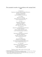
Figure 3: Illustration for the proof of Theorem 4.8 showing a deterministic walk on the five-
dimensional hypercube Q
5
. The walk starts at 00000 and all rotor sequences are ordered
lexicographically.
the electronic journal of combinatorics 17 (2010), #R167 23

the rotor sequences differently, that is, let all rotor sequences be ordered lexicographically
and let the walk start at 0
d
. We bound the time to reach 1
d
. The choice of rotor sequence
yields that every vertex x first visits the neighboring vertices y with |y|
1
< |x|
1
and then
the neighboring vertices y with |y|
1
> |x|
1
. The resulting walk can be nicely described as
a sequence of depth-first-searches (DFS) on a tree T
d
which is a subgraph of Q
d
. The root
of T
d
is 0
d
. In level i there are only vertices x with |x|
1
= i. Every vertex x has either
0 or |x|
0

children corresponding to neighbors y of x with |y|
1
= |x|
1
+ 1. The root has d
children. All other vertices x have |x|
0
children iff the single bit in which it differs from its
parent is left of the leftmost 1-bit. That is, the tree is truncated if the bit which is flipped
from the parent to the child is not a leading zero. Note that this implies that on level i
there are i copies of each vertex with |x|
1
= i in T
d
and only the leftmost recurses to the
next level. Figure 3 on page 23 shows the deterministic walk on Q
5
and the corresponding
tree T
5
as defined above.
We decompose the deterministic walk on Q
d
in d phases such that phase i has length
2

i
j=1
j


d
j

and show the the following:
(i) Initially, the rotors corresponding to the vertices in T
d
point towards their respective
parent.
(ii) After the i-th phase, all rotors of vertices x with |x|
1
> i point towards their
respective parent in T
d
while all rotors of vertices x with |x|
1
 i point to their
leftmost child in T
d
, i.e., to their lexicographic smallest neighbor with one more bit
set to one.
(iii) The i-th phase of the deterministic walk on Q
d
visits the same vertices in the same
order as a DFS on T
d
with limited depth i.
(iv) T
d
has i


d
i

vertices on level i with i > 0.
(i) holds by definition of T
d
for the chosen rotor sequence. We now prove simultaneously
(ii) and (iii) by induction. For the first phase of 2d steps it is easy to see as it alternates
between 0
d
and all nodes x with |x|
1
= 1 (in increasing order). This phase ends at the
root 0
d
whose rotor then points at 0
d−1
1 (as initially). The rotors of nodes x with |x|
1
= 1
now point to the lexicographically smallest neighbor y with |y|
1
= 2. Note that for every
vertex y with |y|
1
= 2 there are two vertices x with |x|
1
= 1 whose rotor points to y. Let
us now assume (ii) and (iii) holds after the i-th phase. Then all rotors of vertices x with
|x|

1
 i point downwards in T
d
to their leftmost child which is also the lexicographically
smallest. It is obvious that then the deterministic walk on Q
d
exactly performs a DFS of
limited depth i + 1 on Q
d
up to the point when a vertex is visited the second time within
this phase. If this vertex x is in the last visited layer, i.e., |x| = i+1, then its rotor points
upwards and the DFS is not disturbed. If a vertex x with |x|  i is visited the second
time, then by definition of T
d
, this vertex has no children. Hence the DFS in T
d
goes back
to its parent which is the same vertex to which the deterministic walk in Q
d
moves as
the rotor is already pointing at its second neighbor in its rotor sequence. The same holds
for the third, fourth, and so on visit to a vertex. Overall, this (i + 1)-st phase visits all
vertices in T
d
up to depth (i + 1) and changes the rotors of vertices x with |x|
1
= (i + 1)
downwards. This proves (ii) and (iii). (iv) immediately follows from the fact that there
the electronic journal of combinatorics 17 (2010), #R167 24
are i copies of each vertex x with |x|

1
= i on level i in T
d
.
The number of vertices visited in phase i with i < d is twice the number of edges up
to depth i. Therefore the length of phase i < d is 2

i
j=1
j

d
j

and the total length of the
deterministic walk on Q
d
until 1
d
is discovered is
d + 1 + 2
d−1

i=0
i

j=1
j

d

j

= d + 1 + 2
d

j=0
j (d − j)

d
j

= d + 1 + 2d
d−1

j=0
j

d−1
j

= d + 1 + d (d − 1) 2
d−1
= (n log
2
n)/2 + O(n log n).
5 Short Term Behavior
For random walks, Barnes and Feige [7, 8] examined how quickly a random walk covers
a certain number of vertices and/or edges. Table 4 provides an overview of their bounds
compared to ours. For the deterministic walk, we can show the following result about the
rate at which the walk discovers new edges in the short term.

Theorem 5.1. All deterministic walks with κ = 1 visit N distinct vertices within
min {O(N∆ + (N∆/δ)
2
), O(m + (m/δ)
2
)} steps and M distinct edges within O(M +
(M/δ)
2
) steps.
The proof of Theorem 5.1 is based on some combinatorial properties of the determin-
istic walk. Let us first observe a simple graph-theoretic lemma.
Lemma 5.2. For any graph G = (V, E), vertex v ∈ V , and i  0 with Γ
i+1
(v) = ∅, we
have
|E(Γ
i
(v)) ∪ E(Γ
i+1
(v)) ∪ E(Γ
i+2
(v))|  δ
2
/6.
Proof. Fix a vertex u ∈ Γ
i+1
(v). Clearly, there exists a j ∈ {i, i + 1, i + 2} such
that |E(u, Γ
j
(v))|  δ/3. Since this implies that |Γ

j
(v)|  δ/3, we have |E(Γ
j
(v))| 
|Γ
j
(v)|δ/2  δ
2
/6 and the claim follows.
In the proof of Theorem 5.1 we will also need the following property borrowed from
Yanovski et al. [54].
Lemma 5.3. For any time t and edges {u, v}, {v, w} ∈ E it holds that
|

N
t
(u → v) −

N
t
(v → w)|  2.
Proof of Theorem 5.1. We start with the second claim. Assume that there is an edge
e = (u, v) ∈ E with

N
t
(e)  13
√
t /δ. Then we know that for all adjacent edges e


= (v, w)
that

N
t
(e

)  13
√
t /δ − 2 as |

N
t
(e) −

N
t
(e

)|  2 by [54, Cor. 4]. More generally, for an
edge e = (x, y) with dist(u, x) = i we have

N
t
(x → y)  13
√
t /δ − 2i. (11)
the electronic journal of combinatorics 17 (2010), #R167 25