Báo cáo toán học: "Combinatorics of the three-parameter PASEP partition function" docx
Bạn đang xem bản rút gọn của tài liệu. Xem và tải ngay bản đầy đủ của tài liệu tại đây (351.33 KB, 31 trang )
Combinatorics of the three-parameter
PASEP partition function
Matthieu Josuat-Verg`es
∗
Universit´e Paris-sud and LRI,
91405 Orsay CEDEX, FRANCE.
Submitted: Jan 23, 2010; Accepted: Jan 10, 2011; Published: Jan 19, 2011
Mathematics Subject Classifications: 05A15, 05A19, 82B23, 60C05.
Abstract
We consider a partially asymmetric exclusion process (PASEP) on a finite num-
ber of sites with open and directed bound ary conditions. Its partition function was
calculated by Blythe, Evans, Colaiori, an d Essler. It is know n to be a generating
function of permutation tableaux by the combinatorial interp retation of Corteel and
Williams.
We prove bijectively two new combinatorial interpretations. The first one is
in terms of weighted Motzkin paths called Laguerre histories and is obtained by
refining a bijection of Foata and Zeilberger. Secondly we show that this partition
function is the generating function of permutations with respect to right-to-left
minima, right-to-left m axima, ascents, and 31-2 patterns, by refining a bijection of
Fran¸con and Viennot.
Then we give a new formula for the partition function which generalizes the
one of Blythe & al. It is proved in two combinatorial ways. The first proof is
an enumeration of lattice paths which are known to be a solution of the Matrix
Ansatz of Derrida & al. The second proof relies on a previou s enumeration of rook
placements, which appear in the combinatorial interpretation of a related normal
ordering p roblem. We also obtain a closed formula for the moments of Al-Salam-
Chihara polynomials.
1 Introduction
1.1 The PASEP p artition function
The partially asymmetric simple exclusion process (also called PASEP) is a Markov chain
describing the evolution of particles in N sites arranged in a line, each site being either
∗
Partially supported by the grant ANR08-JCJC- 0011.
the electronic journal of combinatorics 18 (2011), #P22 1
empty or occupied by one particle. Particles may enter the leftmost site at a rate α ≥ 0,
go out the rightmost site at a rate β ≥ 0, hop left at a rate q ≥ 0 and hop right at a rate
p > 0 when possible. By rescaling time it is always possible to assume that the latter
parameter is 1 without loss of generality. It is possible to define either a continuous-time
model or a discrete-time model, but they are equivalent in the sense that their stationary
distributions are the same. In this article we only study some combinatorial pro perties
of the partition function. For precisions, background about the model, and much more,
we refer to [5, 6, 11, 12, 16, 30]. We refer particularly to the lo ng survey of Blythe and
Evans [4] and all references therein to give evidence that this is a widely studied model.
Indeed, it is quite rich and some important features are the various phase transitions, and
spontaneous symmetry breaking for example, so that it is considered as a fundamental
model of nonequilibrium statistical physics.
A method to obtain the stationary distribution and the partition function Z
N
of the
model is the Matrix Ansatz of Derrida, Evans, Hakim and Pasquier [16]. We suppose that
D and E are linear operators, W | is a vector, |V is a linear form, such that:
DE − qED = D + E, W |αE = W |, βD|V = |V , W |V = 1, (1)
then the non- no rmalized probability of each state can be obtained by taking the product
W |t
1
. . . t
N
|V where t
i
is D if the ith site is occupied and E if it is empty. It follows that
the normalization, or partition function, is given by W |(D + E)
N
|V . It is possible to
introduce another variable y, which is not a parameter of the probabilistic model, but is
a formal parameter such that the coefficient of y
k
in the partition function corresp onds to
the states with exactly k particles (physically it could be called a fugacity). The partition
function is then:
Z
N
= W |(yD + E)
N
|V , (2)
which we may ta ke as a definition in the combinatorial point of view of this article (see
Section 2 below for precisions). An interesting property is the symmetry:
Z
N
α, β, y, q
= y
N
Z
N
β, α,
1
y
, q
, (3)
which can be seen on the physical point of view by exchanging the empty sites with
occupied sites. It can also be obtained from the Matrix Ansatz by using the transposed
matrices D
∗
and E
∗
and the transposed vectors V | and |W , which satisfies a similar
Matrix Ansatz with α and β exchanged.
In section 4, we will use an explicit solution of the Matrix Ansatz [5, 6, 16], and it will
permit to make use of weighted lattice paths as in [6].
1.2 Combinatorial interpretations
Corteel and Williams showed in [11, 12] that the stationary distribution of the PASEP
(and consequently, the partition function) has a natura l combinatorial interpretation in
terms of permutation tableaux [32]. This can be done by showing that the two operators
the electronic journal of combinatorics 18 (2011), #P22 2
D and E of the Matrix Ansatz describe a recursive construction of these objects. They
have in particular:
Z
N
=
T ∈P T
N+1
α
−a(T )
β
−b(T )+1
y
r(T )−1
q
w(T )
, (4)
where P T
N+1
is the set of permutation tableaux of size N + 1, a(T ) is the number of 1s
in the first row, b(T ) is the number of unrestricted rows, r(T ) is the number of rows, and
w(T ) is the number of superfluous 1s. See Definition 3 .1 .1 below, and [12, Theorem 3.1]
for the original statement. Permutation tableaux a r e interesting because of their link
with permutations, and it is po ssible to see Z
N
as a generating function of permutations.
Indeed thanks to the Steingr´ımsson-Williams bijection [32], it is also known that [12]:
Z
N
=
σ∈S
N+1
α
−u(σ)
β
−v(σ)
y
wex(σ)−1
q
cr(σ)
, (5)
where we use the statistics in the following definition.
Definition 1.2.1. Let σ ∈ S
n
. Then:
• u(σ) the number of special right-to-left minima, i.e. integers j ∈ {1, . . . , n} such
that σ(j) = min
j≤i≤n
σ(i) and σ( j) < σ(1),
• v(σ) is the number of special left-to-right maxima, i.e. integers j ∈ {1, . . . , n} such
that σ(j) = max
1≤i≤j
σ(i) and σ(j) > σ(1),
• wex(σ) is the number of weak exceedances of σ, i.e. integers j ∈ {1, . . . , n} such
that σ(j) ≥ j,
• and cr(σ) is the number of crossings, i.e. pairs (i, j) ∈ {1, . . . , n}
2
such t hat either
i < j ≤ σ(i) < σ(j) or σ(i) < σ(j) < i < j.
It can already be seen that Stirling numbers and Eulerian numbers appear as special
cases of Z
N
. We will show that it is po ssible to follow the statistics in (5) through the
weighted Motzkin paths called Laguerre histories (see [9, 33] and Definition 3.1.2 below),
thanks to t he bijection of Foata and Zeilberger [9, 19 , 29]. But we need to study several
subtle properties of the bijection to follow all four statistics. We obtain a combinatorial
interpretation of Z
N
in terms o f Laguerre histories, see Theorem 3.2.4 below. Even more,
we will show that the four statistics in Laguerre histories can be followed through the
bijection of Fran¸con and Viennot [9, 20]. Consequently we will obtain in Theorem 3.3 .3
below a second new combinatorial interpretation:
Z
N
=
σ∈S
N+1
α
−s(σ)+1
β
−t(σ)+1
y
asc(σ)−1
q
31-2(σ)
, (6)
where we use the statistics in the next definition. This was already known in the case
α = 1, see [9, 10].
the electronic journal of combinatorics 18 (2011), #P22 3
Definition 1.2.2. Let σ ∈ S
n
. Then:
• s(σ) is the number of right-to-left maxima of σ and t(σ) is the number of r ig ht-to-left
minima of σ,
• asc(σ) is the number of ascents, i.e. integers i such that either i = n or 1 ≤ i ≤ n−1
and σ(i) < σ(i + 1),
• 31-2(σ) is the number of generalized patterns 31-2 in σ, i.e. triples of integers
(i, i + 1, j) such tha t 1 ≤ i < i + 1 < j ≤ n and σ(i + 1) < σ(j) < σ(i).
1.3 Exact formula for the partition function
An exact formula for Z
N
was given by Blythe, Evans, Colaiori, Essler [5, Equation ( 57)]
in the case where y = 1. It was obtained from the eigenvalues and eigenvectors of the
operator D + E as defined in (16) and (17) below. This method gives an integral form for
Z
N
, which can be simplified so as to obtain a finite sum rather than an integral. Moreover
this expression for Z
N
was used to obtain various properties of the large system size limit,
such a s phases diagra ms and currents. Here we generalize this result since we also have
the variable y, and the proofs are combinatorial. This is a n important result since it is
generally accepted that most interesting properties of a model can be derived from the
partition function.
Theorem 1.3.1. Let ˜α = (1 −q)
1
α
− 1 and
˜
β = (1 −q)
1
β
− 1. We have:
Z
N
=
1
(1 −q)
N
N
n=0
R
N,n
(y, q)B
n
(˜α,
˜
β, y, q), (7)
where
R
N,n
(y, q) =
⌊
N−n
2
⌋
i=0
(−y)
i
q
(
i+1
2
)
n+i
i
q
N−n−2i
j=0
y
j
N
j
N
n+2i+j
−
N
j−1
N
n+2i+j+1
(8)
and
B
n
(˜α,
˜
β, y , q) =
n
k=0
n
k
q
˜α
k
(y
˜
β)
n−k
. (9)
In the case where y = 1, one sum can be simplified by the Vandermonde identity
j
N
j
N
m−j
=
2N
m
, and we recover the expression given in [5, Equation (54)] by Blythe
& al:
R
N,n
(1, q) =
⌊
N−n
2
⌋
i=0
(−1)
i
2N
N−n−2i
−
2N
N−n−2i−2
q
(
i+1
2
)
n+i
i
q
. (10)
the electronic journal of combinatorics 18 (2011), #P22 4
In the case where α = β = 1, it was known [14, 23] that (1 −q)
N+1
Z
N
is equal to:
N+1
k=0
(−1)
k
N+1−k
j=0
y
j
N+1
j
N+1
j+k
−
N+1
j−1
N+1
j+k+1
k
i=0
y
i
q
i(k+1−i)
(11)
(see Remarks 4.3.3 and 5.0.6 for a comparison between this previous result and the new
one in Theorem 1.3.1). And in the case where y = q = 1, from a recursive construction
of permutation tableaux [10] or lattice paths combinatorics [6] it is known that :
Z
N
=
N−1
i=0
1
α
+
1
β
+ i
. (12)
The first proof of (7) is a purely combinatorial enumeration of some weighted Motzkin
paths defined below in (19), appearing from explicit representations of the operato rs D and
E of t he Matrix Ansatz. It partially relies on results of [14, 23] through Proposition 4.1.1
below. In contrast, the second proo f does not use a particular representation of the
operators D and E, but only on the combinatorics of the normal ordering process. It also
relies on previous r esults of [23] (through Proposition 5.0.4 below), but we will sketch a
self-contained proof.
This article is organized as f ollows. In Section 2 we recall known facts about the
PASEP partition function Z
N
, mainly to explain the Matrix Ansatz. In Section 3 we
prove the two new combinatorial interpretations of Z
N
, starting from (5) and using various
properties of bijections of Foata and Zeilberger, Fran¸con and Viennot. Sections 4 and 5
respectively contain the t he two proofs of the exact formula for Z
N
in Equation (7). In
Section 6 we show that the first proof of the exact formula for Z
N
can b e adapted to
give a formula for the moments of Al-Salam- Chihara polynomials. Finally in Section 7 we
review the numerous classical integer sequences which appear as specializations or limit
cases of Z
N
.
Acknowledg ement
I thank my advisor Sylvie Corteel for her advice, support, help and kindness. I thank
Einar Steingr´ımsson, Lauren Williams and Jiang Zeng for their help.
2 Some known properties of the partition function Z
N
As said in the introduction, the partition function Z
N
can be derived by taking the product
W |(yD + E)
N
|V provided the relations (1) are satisfied. It may seem non-obvious that
W |(yD + E)
N
|V does not depend on a part icular choice of the operators D and E, and
the existence of such operators D and E is not clear.
The fact that W |(yD + E)
N
|V is well-defined without making D and E explicit,
in a consequence of the existence of normal forms. More precisely, via the commutation
the electronic journal of combinatorics 18 (2011), #P22 5
relation DE −qED = D +E we can derive polynomials c
(N)
i,j
in y and q with non-negative
integer coefficients such that we have the normal form:
(yD + E)
N
=
i,j≥0
c
(N)
i,j
E
i
D
j
(13)
(this is a finite sum). See [3] for other combinatorial interpretation of normal ordering
problems. It turns out that the c
(N)
i,j
are uniquely defined if we require the previous equality
to hold for any value of α, β, y and q, considered as indeterminates. Then the partition
function is:
Z
N
(α, β, y, q) = W |(yD + E)
N
|V =
i,j≥0
c
(N)
i,j
α
−i
β
−j
. (14)
Indeed, this expression is valid for any choice of W |, |V , D and E since we only used
the relations (1) to obtain it. In particular Z
N
is a polynomial in y, q,
1
α
and
1
β
with
non-negative coefficients. For convenience we also define:
¯
Z
N
α, β, y, q
= Z
N
1
α
,
1
β
, y, q
. (15)
For example the first values are:
¯
Z
0
= 1,
¯
Z
1
= α + y β,
¯
Z
2
= α
2
+ y(α + β + αβ + αβq) + y
2
β
2
,
¯
Z
3
= y
3
β
3
+
αβ
2
q + αβ
2
+ α + αβ + αβ
2
q
2
+ β + β
2
q + 2 aβq + 2β
2
y
2
+
2α
2
+ α
2
q + α + βα
2
q
2
+ βα
2
+ βα
2
q + αβ + β + 2αβq
y + α
3
.
Even if it is not needed to compute the first values of Z
N
, it is useful to have explicit
matrices D and E satisfying (1). The best we could hope is finite-dimensional matrices
with non-negative entries, however this is known to be incompatible with the existence
of phase transitions in the model (see section 2.3.3 in [4]). Let ˜α = (1 − q)
1
α
− 1 and
˜
β = (1 − q)
1
β
− 1, a solution of the Matrix Ansatz (1) is given by the following matrices
D = (D
i,j
)
i,j∈N
and E = (E
i,j
)
i,j∈N
(see [16]):
(1 −q)D
i,i
= 1 +
˜
βq
i
, (1 − q)D
i,i+1
= 1 − ˜α
˜
βq
i
, (16)
(1 −q)E
i,i
= 1 + ˜αq
i
, (1 − q) E
i+1,i
= 1 −q
i+1
, (17)
all other coefficients being 0, and vectors:
W | = (1, 0, 0, . . . ), |V = (1, 0, 0, . . . )
∗
, (18)
(i.e. |V is the transpose of W | ) . Even if infinite-dimensional, they have the nice property
of being tridiagonal and this lead to a combinatorial interpretation of Z
N
in terms of lattice
paths [6]. Indeed, we can see yD + E as a transfer matrix for walks in the non-negative
the electronic journal of combinatorics 18 (2011), #P22 6
integers, and obtain that (1 −q)
N
Z
N
is the sum of weights of Motzkin paths of length N
with weights:
• 1 − q
h+1
for a step ր starting at height h,
• (1 + y) + (˜α + y
˜
β)q
h
for a step → starting at height h,
• y(1 − ˜α
˜
βq
h−1
) for a step ց starting at height h.
(19)
We recall that a Motzkin path is similar to a Dyck path except that there may be hori-
zontal steps, see Figures 1, 3, 4, 5 further. These weighted Motzkin paths are our starting
point to prove Theorem 1.3.1 in Section 4.
We have sketched how the Motzkin paths appear as a combinatorial interpretat io n of
Z
N
starting from the Matrix Ansatz. However it is also possible to obta in a direct link
between the PASEP and the lattice paths, independently of the results of Derrida & al.
This was done by Brak & a l in [6], in the even more general context of the PASEP with
five parameters.
3 Combinatorial interpretations of Z
N
In this section we prove the two new combinatorial interpretation of Z
N
. Firstly we prove
the one in terms o f Laguerre histories (Theorem 3.2.4 below), by means of a bijection orig-
inally given by Foata and Zeilberger. Secondly we prove the one in terms in permutations
(Theorem 3.3.3 below).
3.1 Permutation tableaux and Laguerre histories
We recall here t he definition of permutation tableaux and their statistics needed to state
the previously known combinatorial interpretation (4).
Definition 3.1.1 ([32]). Let λ be a Young diagram (in English notation), possibly with
empty rows but with no empty column. A complete filling of λ with 0 ’s and 1’s is a
permutation tableau if:
• for any cell containing a 0, all cells above in the same column contain a 0, or all
cells to the left in the same row contain a 0,
• there is at least a 1 in each column.
A cell containing a 0 is restricted if there is a 1 above. A row is restricted if it contains
a restricted 0, and unrestricted otherwise. A cell containing a 1 is essential if it is the
topmost 1 of its column, otherwise it is superfluous. The size of such a permutatio n
tableaux is the number of rows of λ plus its number of columns.
the electronic journal of combinatorics 18 (2011), #P22 7
To prove our new combinatorial interpretations, we will give bijections linking the
previously-known combinatorial interpretation (5), and t he new ones. The main combi-
natorial object we use a re the Laguerre histories, defined below.
Definition 3.1.2 ([33]). A Laguerre history of size n is a weighted Motzkin path of n
steps such that:
• the weight of a step ր starting at height h is yq
i
for some i ∈ {0, . . . , h},
• the weight o f a step → starting at height h is either yq
i
for some i ∈ {0, . . . , h} or
q
i
for some i ∈ {0, . . . , h − 1},
• the weight of a step ց starting at height h is q
i
for some i ∈ {0, . . . , h − 1}.
The total weight of the Laguerre history is the product of the weights of its steps. We call
a type 1 step , any step having weight yq
h
where h is its starting height. We call a type 2
step, any step having weight q
h−1
where h is its starting height.
As shown by P. Flajolet [18], the weighted Motzkin paths appear in various combi-
natorial contexts in connexion with some continued fractions called J-fractions. We also
recall an important fact fro m combinatorial theory of orthogonal polynomials.
Proposition 3.1.3 (Flajolet [18], Viennot [33]). If an orthogonal sequence {P
n
}
n∈N
is
defined by the three-term recurrence relation
xP
n
(x) = P
n+1
(x) + b
n
P
n
(x) + λ
n
P
n−1
(x), (20)
then the moment generating function has the J-fraction representation
∞
n=0
µ
n
t
n
=
1
1 −b
0
t −
λ
1
t
2
1 −b
1
t −
λ
2
t
2
.
.
.
, (21)
equivalently the nth moment µ
n
is the sum of weights of Motzkin paths of length n whe re
the weight of a step ր (respectivel y →, ց) starting at height h is a
h
(respectively b
h
, c
h
)
provided λ
n
= a
n−1
c
n
.
Remark 3.1.4. The sum of weights of Laguerre histories of length n is the nth mo-
ment of some q-Laguerre polynomials (see [25]), which are a special case of rescaled
Al-Salam-Chihara polynomials. On the other hand Z
N
is the N th moment o f shifted Al-
Salam-Chihara po lynomials (see Section 6). We will use the Laguerre histories to derive
properties of Z
N
, however they are related with two different orthogonal sequences.
the electronic journal of combinatorics 18 (2011), #P22 8
3.2 The Foata-Zeilberger bijection
Foata and Zeilberger gave a bijection between permutations and Laguerre histories in [19].
It has been extended by de M´edicis and Viennot [29], and Corteel [9]. In particular, Corteel
showed that through this bijection Ψ
F Z
we can follow the number weak exceedances and
crossings [9]. The bijection Ψ
F Z
links permutations in S
n
and Laguerre histories of n
steps. The ith step of Ψ
F Z
(σ) is:
• a step ր if i is a cycle valley, i.e. σ
−1
(i) > i < σ(i),
• a step ց if i is a cycle peak, i.e. σ
−1
(i) < i > σ(i),
• a step → in a ll other cases.
And the weight of the ith step in Ψ
F Z
(σ) is y
δ
q
j
with:
• δ = 1 if i ≤ σ(i) and 0 otherwise,
• j = #{ k | k < i ≤ σ (k) < σ(i) } if i ≤ σ(i),
• j = #{ k | σ( i) < σ(k) < i < k } if σ(i) < i.
It follows that the total weight of Ψ
F Z
(σ) is y
wex(σ)
q
cr(σ)
. To see the statistics wex and
cr in a permutation σ, it is practical to represent σ by an arrow diagram. We draw n
points in a line, and draw an arrow from the ith point to the σ(i)th point for a ny i. This
arrow is above the axis if i ≤ σ(i), below the axis otherwise. Then wex(σ) is the number
of ar rows above the axis, and cr(σ) is the number of proper intersection between arr ows
plus the number of chained a rr ows going to t he right. See Fig ure 1 for an example with
σ = 672581493, so that wex(σ) = 5 and cr(σ) = 7.
yq
0
yq
1
q
0
yq
0
yq
3
q
2
q
0
yq
1
q
0
Figure 1: The permutation σ = 6725814 93 and its image Ψ
F Z
(σ).
Lemma 3.2.1. Let σ ∈ S
n
, and 1 ≤ i ≤ n. Then i is a left-to-right maximum of σ if
and o nly if the ith step of Ψ
F Z
(σ) is a type 1 step (as in Definition 3.1.2).
Proof. Let us call a (σ, i)-sequence a strictly increasing maximal sequence of integers
u
1
, . . . , u
j
such that σ(u
k
) = u
k+1
for any 1 ≤ k ≤ j − 1, and also such that u
1
< i < u
j
.
By maximality of the sequence, u
1
is a cycle valley and u
j
is a cycle peak. The number
of such sequences is the difference between the number of cycle valleys and cycle peaks
among {1, . . . , i −1}, so it is the starting height h of the ith step in Ψ
F Z
(σ).
the electronic journal of combinatorics 18 (2011), #P22 9
Any left-to-right maximum is a weak exceedance, so i is a left-to-right maxima of σ
if and only if i ≤ σ(i) and there exists no j such that j < i ≤ σ(i) < σ(j). This is also
equivalent t o the f act that i ≤ σ(i), and there exists no two consecutive elements u
k
, u
k+1
of a (σ, i)- sequence such that u
k
< i ≤ σ(i) < u
k+1
. This is also equivalent to the fact
that i ≤ σ(i), and any (σ, i)-sequence contains two consecutive elements u
k
, u
k+1
such
that u
k
< i ≤ u
k+1
< σ(i).
By definition of the bijection Ψ
F Z
it is equivalent to the fact that the ith step of
Ψ
F Z
(σ) has weight yq
h
, i.e. the ith step is a type 1 step.
Lemma 3.2.2. Le t σ ∈ S
n
, an d 1 ≤ i ≤ n. We suppose i = σ(i). Then i is a right-to-left
minima of σ if and only if the ith step of Ψ
F Z
(σ) is a type 2 step.
Proof. We have to pay attention to the fact that a right-to-left minimum can be a fixed
point and we only characterize the non-fixed points here. This excepted, the proof is
similar to the one of the previous lemma.
Before we can use the bijection Ψ
F Z
we need a slight modification of the known
combinatorial interpretation (5), given in the following lemma.
Lemma 3.2.3. We have:
¯
Z
N
=
σ∈S
N+1
α
u
′
(σ)
β
v(σ)
y
wex(σ)−1
q
cr(σ)
, (22)
where u
′
(σ) is the number of right-to-left minima i of σ satisfying σ
−1
(N + 1) < i.
Proof. This just means that in (5) we can replace the statistic u with u
′
, and this can
be done via a simple bijection. For any σ ∈ S
N+1
, let ˜σ be the reverse complement o f
σ
−1
, i.e. σ(i) = j if and only if ˜σ(N + 2 − j) = N + 2 − i. It is routine to check that
u(σ) = u
′
(˜σ), wex(σ) = wex(˜σ), and v(σ) = v(˜σ). Moreover, one can check that the arrow
diagram of ˜σ is obtained from the one of σ by a vertical symmetry and arrow reversal, so
that cr(σ) = cr(˜σ). So (5) and the bijection σ → ˜σ prove (22).
From Lemmas 3.2.1, 3.2.2, and 3.2.3 it possible to give a combinatorial interpretation
of
¯
Z
N
in terms of the Laguerre histories. We start from the statistics in S
N+1
described
in Definition 1.2.1, t hen fr om (22) and the properties of Ψ
F Z
we obtain the following
theorem.
Theorem 3.2.4. The polynomial y
¯
Z
N
is the generating function of Laguerre histories of
N + 1 steps, where:
• the parameters y and q are given by the total wei ght of the path,
• β counts the type 1 steps, except the first one,
• α counts the type 2 steps whic h are to the right of any type 1 s tep.
the electronic journal of combinatorics 18 (2011), #P22 10
Proof. Let σ ∈ S
N+1
. The smallest left-to-right maximum of σ is 1, and any other left-to-
right maximum i is such that σ(1) < σ(i). So 1 is the only left-to-right maximum which
is not special. So by Lemma 3.2.1, v(σ) is the number o f type 1 steps in Ψ
F Z
(σ), minus
1.
Moreover, σ
−1
(N +1) is the largest left-to-right maximum of σ. Let i be a right-to-left
minimum of σ such that σ
−1
(N + 1) < i. We have i = σ(i), otherwise σ would stabilize
the interval {i + 1, . . . , N + 1} and this would contradict σ
−1
(N + 1) < i. So we can apply
Lemma 3 .2 .2, and it comes that u
′
(σ) is the number of type 2 steps in Ψ
F Z
(σ), which a r e
to the right of any type 1 step. So (22) and the bijection Ψ
F Z
prove the theorem.
Before ending this subsection, we sketch how to recover a known result in the case
q = 0 from Theorem 3.2.4. This was given in Section 3.2 of [7] (see also Section 3.6 in
[4]) and proved via generating functions. For any Dyck path D, let ret(D) be t he number
of returns to height 0, for example ret(րց) = 1 and ret(րցրց) = 2, and the empty
path · satisfies ret(·) = 0. The r esult is the following.
Proposition 3.2.5 (Brak, de Gier, Rittenberg). When y = 1 and q = 0, the partition
function is Z
N
=
(
1
β
)
ret(D
1
)
(
1
α
)
ret(D
2
)
where the sum is over pairs of Dyck paths (D
1
, D
2
)
whose lengths sum to 2N.
Proof. When q = 0 we can remove any step with weight 0 in the Laguerre histories. When
y = 1, to distinguish the two kinds of horizontal steps we introduce another kind of paths.
Let us call a bicolor Motzkin path, a Motzkin path with two kinds of horizontal steps
and →, and such that there is no at height 0. From Theorem 3.2.4, if y = 1 and q = 0
then β
¯
Z
N
is the generating function of bicolor Motzkin paths M o f length N + 1, where:
• there is a weight β on each step ր or → starting at height 0,
• there is a weight α o n each step ց or starting at height 1 and being to the right
of any step with a weight β.
There is a bijection between these bicolor Motzkin paths, and Dyck paths of length 2N +2
(see de M´edicis and Viennot [29]). To obtain the Dyck path D, each step ր in the bicolor
Motzkin pat h M is replaced with a sequence of two steps րր. Similarly, each step →
is replaced with րց, each step is replaced with ցր, each step ց is replaced with
ցց. When some step s ∈ {ր, →, ց} in M has a weight β or α, and is transformed into
steps (s
1
, s
2
) ∈ {ր , →, ց}
2
in D, we choose to put the weight β or α on s
1
. It appears
that D is a Dyck path of length 2N + 2 such that:
• there is a weight β on each step ր starting at height 0,
• there is a weight α on each step ց starting at height 2 and being to the right of
any step with weight β.
Then D can be factorized into D
1
ր D
2
ց where D
1
and D
2
are Dyck paths whose
lengths sum to 2N, and up to a factor β it can b e seen that β (respectively α) counts
the electronic journal of combinatorics 18 (2011), #P22 11
the returns to height 0 in D
1
(resp ectively D
2
). More precisely the βs are on the steps ր
starting at height 0 but there are as many of them as the number o f returns to height 0.
See Figure 2 for a an example.
M =
β
β
β
αα
D =
β β β
α α
D
1
=
β β
D
2
=
α α
Figure 2: The bijection between M, D and (D
1
, D
2
).
3.3 The Fran¸con-Viennot bijection
This bijection was given in [20]. We use here the definition of this bijection given in [9].
The map Ψ
F V
is a bijection between permutations of size n and Laguerre histories of n
steps. Let σ ∈ S
n
, j ∈ {1, . . . , n} and k = σ(j). Then the kth step of Ψ
F V
(σ) is:
• a step ր if k is a va lley, i.e. σ(j −1) > σ(j) < σ( j + 1),
• a step ց if k is a peak, i.e. σ(j − 1) < σ(j) > σ(j + 1),
• a step → if k is a double ascent, i.e. σ(j −1) < σ(j) < σ(j + 1), or a double descent,
i.e. σ(j −1) > σ(j) > σ(j + 1).
This is done with the convention that σ(n + 1) = n + 1, in particular n is always an
ascent of σ ∈ S
n
. Moreover the weight of the kt h step is y
δ
q
i
where δ = 1 if j is an
ascent and 0 otherwise, and i = 31-2(σ, j). This number 31-2(σ, j) is the number of
patterns 31-2 such that j correspond to the 2, i.e. integers i such that 1 < i + 1 < j and
σ(i + 1) < σ(j) < σ(i). A consequence of the definition is that the total weight of Ψ
F V
(σ)
is y
asc(σ)
q
31-2(σ)
. See Figures 3 and 4 for examples.
1
2
3
4
5
6
7
1 2 3 4 5 6 7
yq
0
yq
1
yq
0
q
0
yq
1
q
1
q
0
Figure 3: Example of the permutation 4 371265 and its imag e by the Fran¸con-Viennot
bijection.
the electronic journal of combinatorics 18 (2011), #P22 12
Lemma 3.3.1. Let σ ∈ S
n
and 1 ≤ i ≤ n. Then σ
−1
(i) is a right-to-left mi nimum of σ
if and only if the ith step of Ψ
F V
(σ) is a type 1 step.
Proof. This could be done by combining the arguments of [20] and [9]. We sketch a proof
introducing ideas that will be helpful for the next lemma.
We suppose that j = σ
−1
(i) is a right-to-left minimum. So j is an ascent, and any v
such that i > σ(v) is such that v < j. The integer 31-2(σ, j) is the number of maximal
sequence of consecutive integers u, u + 1, . . . , v such that σ(u) > σ(u + 1) > ··· > σ(v),
and σ(u) > i > σ(v). Indeed, any o f these sequences u, . . . , v is such that v < j and
so it is possible to find two consecutive elements k, k + 1 in the sequence such that
σ(k + 1) < σ(j) < σ(k), and these k, k + 1 only b elong to o ne sequence.
We call a (σ, i)-sequence a maximal sequence of consecutive integers u, u + 1, . . . , v
such that σ(u) > σ ( u + 1) > ··· > σ(v ) , and σ(u) ≥ i > σ(v) . By maximality, u is a peak
and v is a valley. The number of such sequences is the difference between the number
of peaks and number of valleys among the elements of image smaller than i, so it is the
starting height h of the ith step in Ψ
F V
(σ).
So with this definition, we can check that j = σ
−1
(i) is a right-to-left minimum of σ
if and only if j is an ascent and any (σ, i)-sequence u, u + 1, . . . , v is such that v < j. So
this is equivalent to the fact that the ith step of Ψ
F V
(σ) is a type 1 step.
Lemma 3.3.2. Let σ ∈ S
n
, and 1 ≤ i ≤ n. We suppose σ
−1
(i) < n. Then σ
−1
(i) is a
right-to-left maximum of σ if an d only if
• the ith step of Ψ
F V
(σ) it is a type 2 step,
• any type 1 step is to the le f t o f the ith step.
Proof. We keep t he definition of (σ, i)-sequence as in t he previous lemma. First we suppose
that σ
−1
(i) is a right-to-left maximum strictly smaller than n, and we check that the two
points are satisfied. If σ
−1
(j) is a right-to- left minimum, then i > j, so the second point
is satisfied. A right-to-left maximum is a descent, so the ith step is → or ց with weight
q
g
. We have to show g = h − 1. Since σ
−1
(i) is a right-to-left maximum, there is no
(σ, i)-sequence u < ··· < v with σ
−1
(i) < u. So there is one (σ, i)- sequence u < ··· < v
such that u ≤ σ
−1
(i) < v, and the h −1 other ones contains o nly integers strictly smaller
than σ
−1
(i). So the ith step of Ψ
F V
(σ) has weight q
h−1
.
Reciprocally, we suppose that the two p oints above are satisfied. There are h−1 (σ, i)-
sequence containing integers strictly smaller than σ
−1
(i). Since σ
−1
(i) is a descent, the
hth (σ, i)-sequence u < ··· < v is such that u ≤ σ
−1
(i) < v. So there is no (σ, i)-sequence
u < ··· < v such that σ
−1
(i) < u.
If we suppose that i is not a right-to-left maximum, t here would exist k > i such that
σ
−1
(k) > σ
−1
(i). We take the minimal k satisfying this property. Then the images of
σ
−1
(k) + 1 , . . . , n are strictly greater than k, otherwise there would exist ℓ > σ
−1
(k) such
that σ(ℓ) > i > σ ( ℓ + 1). But then σ
−1
(k) would be a right-to-left minimum and this
would contradict the second point that we assumed to be satisfied.
the electronic journal of combinatorics 18 (2011), #P22 13
In Theorem 3.2.4 we have seen that
¯
Z
N
is a generating function of Laguerre histo-
ries, and the bijection Ψ
F V
together with the two lemmas above give our second new
combinatorial interpretation of
¯
Z
N
.
Theorem 3.3.3. We have:
¯
Z
N
=
σ∈S
N+1
α
s(σ)−1
β
t(σ)−1
y
asc(σ)−1
q
31-2(σ)
, (23)
where we use the statistics in Definition 1.2.2 above.
For example, in Figure 4 we have a permutation σ such that
α
s(σ)−1
β
t(σ)−1
y
asc(σ)−1
q
31-2(σ)
= α
2
β
3
y
5
q
7
.
Indeed Ψ
F V
(H) has t otal weight y
5
q
7
, has four type 1 steps and two type 2 steps to the
right of the type 1 steps.
1
2
3
4
5
6
7
8
9
1 2 3 4 5 6 7 8 9
yq
0
yq
1
yq
1
yq
2
yq
1
q
1
q
1
q
0
q
0
Figure 4: The permutation σ = 812563974 and its image by Ψ
F V
.
Remark 3.3.4. We have mentioned in the introduction that the non-normalized prob-
ability of a particular state of the PASEP is a product W |t
1
. . . t
N
|V . It is known
[11] that in the combinatorial interpretation (4), this state of the PASEP corresponds to
permutation tableaux of a given shape. It is also known [11] that in the combinatorial
interpretation (5), this state of the PASEP correspo nds to permutations with a given set
of weak exceedances (namely, i + 1 is a weak exceedance if and only if t
i
= D, i.e. the ith
site is occuppied). It is also possible to give such criterions for the new combinatorial in-
terpretations of Theorems 3.2.4 and 3.3.3, by following the weak exceedances set through
the bijections we have used. More precisely, in the first case the term W |t
1
. . . t
N
|V
is the generating function of Laguerre histories H such that t
i
= D if and only if the
(N +1−i)th step in H is either a step → with weight yq
i
or a step ց. In the second case,
the term W |t
1
. . . t
N
|V is the generating function of permutations σ such that t
i
= D if
and only if σ
−1
(N + 1 − i) is a double ascent or a peak.
the electronic journal of combinatorics 18 (2011), #P22 14
4 A first combinatorial derivation of Z
N
using lattice
paths
In this section, we give the first proof of Theorem 1.3.1.
We consider the set P
N
of weighted Motzkin paths of length N such that:
• the weight of a step ր starting at height h is q
i
− q
i+1
for some i ∈ {0, . . . , h},
• the weight of a step → starting at height h is either 1 + y or (˜α + y
˜
β)q
h
,
• the weight of a step ց starting at height h is either y or −y ˜α
˜
βq
h−1
.
The sum of weights of elements in P
N
is (1 − q)
N
Z
N
because the weights sum to the
ones in (19). We stress that on the combinatorial point of view, it will be important to
distinguish (h + 1) kinds of step ր starting at height h, instead of one kind of step ր
with weight 1 − q
h+1
.
We will show that each element of P
N
bijectively corresponds to a pair of weighted
Motzkin paths. The first path (respectively, second path) belongs to a set whose generat-
ing function is R
N,n
(y, q) (respectively, B
n
(˜α,
˜
β, y, q)) for some n ∈ {0, . . . , N}. Following
this scheme, our first combinatorial proof of (7) is a consequence of Propositions 4.1.1,
4.2.1, and 4.3.1 below.
4.1 The lattice p aths for R
N,n
(y, q)
Let R
N,n
be the set of weighted Motzkin paths of length N such that:
• the weight of a step ր starting at height h is either 1 or −q
h+1
,
• the weight of a step → starting at height h is either 1 + y or q
h
,
• the weight of a step ց is y,
• there are exactly n steps → weighted by a power of q.
In this subsection we prove the following:
Proposition 4.1.1. The sum of weights of elements in R
N,n
is R
N,n
(y, q).
This can be obtained with the methods used in [14, 23], and the result is a consequence
of the Lemmas 4.1.2, 4.1.3 and 4.1.4 b elow.
Lemma 4.1.2. There is a weight-preserving bijection between R
N,n
, and the pairs (P, C)
such that for some i ∈ {0, . . . , ⌊
N−n
2
⌋},
• P is a Motzkin prefix of length N and final height n + 2i, with a weigh t 1 + y on
every step →, and a weight y on every step ց,
the electronic journal of combinatorics 18 (2011), #P22 15
• C is a Motzkin path of length n + 2i, such that
– the weight of a step ր starting at he i ght h is 1 or −q
h
,
– the weight of a step → starting at he i ght h is q
h
,
– the weight of a step ց is 1 ,
– there are exactly n steps →, and no steps րց both with weights 1.
(24)
Proof. This is a direct adaptation of [14, Lemma 1].
Lemma 4.1.3. The generating function of Motzkin prefixes of length N and final height
n + 2i, with a weight 1 + y on every step →, and a weight y on every step ց, is
N−n−2i
j=0
y
j
N
j
N
n+2i+j
−
N
j−1
N
n+2i+j+1
.
Proof. This was given in [14, Proposition 4].
Lemma 4.1.4. The sum of weights of Motzkin pa ths of length n +2i satisfying properties
(24) above is (−1)
i
q
(
i+1
2
)
n+i
i
q
.
Proof. A bijective proof was given in [23, Lemmas 3, 4].
Some precisions are in order. In [14] and [23], we obtained the f ormula (11) which is
the special case α = β = 1 in Z
N
, and is the Nth moment of the q-Laguerre polynomials
mentioned in Remark 3.1.4. Since Z
N
is also very closely related with these po lynomials
(see Section 6) it is not surprising that some steps are in common between these previous
results and the present ones. See also Remark 4.3.3 below.
4.2 The lattice p aths for B
n
(˜α,
˜
β, y, q)
Let B
n
be the set of weighted Motzkin paths of length n such that:
• the weight of a step ր starting at height h is either 1 or −q
h+1
,
• the weight of a step → starting at height h is (˜α + y
˜
β)q
h
,
• the weight of a step ց starting at height h is −y ˜α
˜
βq
h−1
.
In this section we prove the following:
Proposition 4.2.1. The sum of weights of elements in B
n
is B
n
(˜α,
˜
β, y, q).
the electronic journal of combinatorics 18 (2011), #P22 16
Proof. Let ν
n
be the sum of weights of elements in B
n
. It is homogeneous of degree n
in ˜α and
˜
β since each step → has degree 1 and each pair of steps ր and ց has degree
2. By comparing the weights for paths in B
n
, and the ones in (19), we see that ν
n
is the
term of (1 −q)
n
Z
n
with highest degree in ˜α and
˜
β. Since ˜α and (1 −q)
1
α
(resp ectively,
˜
β
and (1 −q)
1
β
) only differ by a constant, it remains only to show that the term of
¯
Z
n
with
highest degree in α and β is
n
k=0
n
k
q
α
k
(yβ)
n−k
.
This follows from the combinatorial interpretation in Equation (4) in terms of permu-
tation tableaux (see Definition 3.1.1). In the term of
¯
Z
n
with highest degree in α a nd β,
the coefficient of α
k
β
n−k
is obtained by counting permutations tableaux of size n +1, with
n−k +1 unrestricted rows, k 1s in the first row. Such permutation tableaux have n−k +1
rows, k columns, and contain no 0. They are in bijection with the Young diagrams that
fit in a k × (n − k) box and give a factor
n
k
q
.
We can give a second proof in relation with orthogonal polynomials.
Proof. It is a consequence of properties of the Al- Sala m-Carlitz orthogonal po lynomials
U
(a)
k
(x), defined by the recurrence [2, 27]:
U
(a)
k+1
(x) = xU
(a)
k
(x) + (a + 1)q
k
U
(a)
k
(x) + a(q
k
− 1)q
k−1
U
(a)
k−1
(x). (25)
Indeed, from Proposition 3.1.3 the sum of weights of elements in B
n
is the nth moment
of the orthogonal polynomial sequence {P
k
(x)}
k≥0
defined by
P
k+1
(x) = xP
k
(x) + (˜α + y
˜
β)q
k
P
k
+ (q
k
− 1)y ˜α
˜
βq
k−1
P
k−1
. (26)
We have P
k
(x) = (y
˜
β)
k
U
(a)
k
(x(y
˜
β)
−1
) where a = ˜α(y
˜
β)
−1
, and the nth moment of the
sequence {U
(a)
k
(x)}
k≥0
is
k
j=0
k
j
q
a
j
(see §5 in [2], or the article of D. Kim [26, Section 3]
for a combinatorial proof). Then we can derive the moments of {P
k
(x)}
k≥0
, and this gives
a second proof of Proposition 4.2.1.
Another possible proof would be to write the generating function
∞
n=0
ν
n
z
n
as a
continued fra ction with the usual methods [18], use a limit case of identity (19.2.11a) in
[15] to relate this generating function with a basic hypergeometric series and then expand
the series.
4.3 The decomposition of lattice paths
Let R
∗
N,n
be defined exactly as R
N,n
, except that the possible weights of a step ր starting
at height h are q
i
− q
i+1
with i ∈ {0, . . . , h}. The sum of weights of elements in R
∗
N,n
is
the same as with R
N,n
, because the possible weights of a step ր starting at height h sum
to 1 − q
h+1
. Similarly let B
∗
n
be defined exactly as B
n
, except that the possible weights
of a step ր starting at height h are q
i
− q
i+1
with i ∈ {0, . . . , h}.
Proposition 4.3.1. There exists a weight-preserving bijection Φ between the disjoint
union of R
∗
N,n
× B
∗
n
over n ∈ {0, . . . , N}, and P
n
(we understand that the wei ght of a
pair is the product of the weigh ts of each ele ment).
the electronic journal of combinatorics 18 (2011), #P22 17
To define the bijection, we start from a pair (H
1
, H
2
) ∈ R
∗
N,n
× B
∗
n
for some n ∈
{0, . . . , N} and build a path Φ(H
1
, H
2
) ∈ P
N
. Let i ∈ {1, . . . , N}.
• If the ith step of H
1
is a step → weighted by a power of q, say the jth one among
the n such steps, then:
– the ith step Φ(H
1
, H
2
) has the same direction as the jth step of H
2
,
– its weight is the product of weights of the ith step of H
1
and the jth step of
H
2
.
• Otherwise the ith step of Φ(H
1
, H
2
) has the same direction and same weight as the
ith step of H
1
.
See Figure 5 for an example, where the thick steps correspond to the ones in the first of
the two cases considered above. It is immediate that the total weight of Φ(H
1
, H
2
) is the
product of the total weights of H
1
and H
2
.
1 − q
q
q −q
2
q
2
q
2
1 − q
y
y
q
y
q
0
H
1
=
1 − q
(˜α + y
˜
β)q
1 − q
−y ˜α
˜
βq
−y ˜α
˜
β
H
2
=
1 − q
q −q
2
q −q
2
(˜α + y
˜
β)q
3
q
2
− q
3
1 − q
y
y
−y ˜α
˜
βq
2
y
−y ˜α
˜
β
Φ(H
1
, H
2
) =
Figure 5: Example of paths H
1
, H
2
and their image Φ(H
1
, H
2
) .
The inverse bijection is not as simple. Let H ∈ P
N
. The method consists in reading
H step by step from right to left, and building two paths H
1
and H
2
step by step so
that at the end we obtain a pair (H
1
, H
2
) ∈ R
∗
N,n
× B
∗
n
for some n ∈ {0, . . . , N}. At
each intermediate stage, we have built two Motzkin suffixe s , i.e. some paths similar to
Motzkin paths except that the starting height may be non-zero.
Let us fix some notation. Let H
(j)
be the Motzkin suffix obtained by taking the j
last steps o f H. Suppose that we have already read the j la st steps of H, and built two
Motzkin suffixes H
(j)
1
and H
(j)
2
. We describe how to iteratively obtain H
(j+1)
1
and H
(j+1)
2
.
Note that H
(0)
1
and H
(0)
2
are empty paths. Let h, h
′
, and h
′′
be the respective starting
heights of H
(j)
, H
(j)
1
and H
(j)
2
.
This iterative construction will have the following properties, as will be immediate
from the definition below:
the electronic journal of combinatorics 18 (2011), #P22 18
• H
(j)
1
has length j, and t he length of H
(j)
2
is the number of steps → weighted by a
power of q in H
(j)
1
.
• We have h = h
′
+ h
′′
.
• The map Φ as we described it can also be defined in the same way fo r Motzkin
suffixes, and is such that H
(j)
= Φ(H
(j)
1
, H
(j)
2
).
To obtain H
(j+1)
1
and H
(j+1)
2
, we read the (j + 1)th step in H starting from the right, and
add steps to the left of H
(j)
1
and H
(j)
2
according to the following rules:
step read in H step added to H
(j)
1
step added to H
(j)
2
ց −y ˜α
˜
βq
h
→ q
h
′
ց −y ˜α
˜
βq
h
′′
ց y ց y
→ 1 + y → 1 + y
→ (˜α + y
˜
β)q
h
→ q
h
′
→ (˜α + y
˜
β)q
h
′′
ր q
i
− q
i+1
with i < h
′
ր q
i
− q
i+1
ր q
i
− q
i+1
with i ≥ h
′
→ q
h
′
ր q
i−h
′
− q
i+1−h
′
We can also iteratively check the following points.
• With this construction H
(j+1)
1
and H
(j+1)
2
are indeed Motzkin suffixes. This is be-
cause we add a step ր to H
(j)
1
only in the case where i < h
′
, hence h
′
> 0. And
we add a step ր to H
(j)
2
only in the case where i ≥ h
′
, hence h
′′
> 0 (since
h = h
′
+ h
′′
> i).
• The paths H
(j+1)
1
and H
(j+1)
2
are respectively suffixes of an element in R
N,n
and B
n
for some n ∈ {0, . . . , N}, i.e. t he weights are valid.
• The set of rules we have given is the only possible one such that for any j we have
H
(j)
= Φ(H
(j)
1
, H
(j)
2
).
It follows that (H
(N)
1
, H
(N)
2
) ∈ R
∗
N,n
× B
∗
n
for some n ∈ {0, . . . , N}, these paths are such
that Φ(H
(N)
1
, H
(N)
2
) = H, and it is the only pair of paths satisfying these properties. There
are details to check, but we have a full description of Φ and of the inverse map Φ
−1
. See
Figure 6 for an example of the Motzkin suffixes we consider.
Before ending this subsection we can mention another argument to show that P
N
and
the disjoint union of R
∗
N,n
×B
∗
n
have the same cardinal. Thus we could just focus on the
surjectivity of the map Φ and avoid making t he inverse map explicit. The argument uses
the electronic journal of combinatorics 18 (2011), #P22 19
q −q
2
−y ˜α
˜
βq
2
(˜α + y
˜
β)q
2
y
−y ˜α
˜
β
H
(j)
=
q
1
q
1
q
1
y
q
0
H
(j)
1
=
1 − q
−y ˜α
˜
βq
(˜α + y
˜
β)q
−y ˜α
˜
β
H
(j)
2
=
Figure 6: Example of Motzkin suffixes used to define Φ
−1
.
the notion of histories [33] and t heir link with classical combinatorial objects, as we have
seen in the previous section with Laguerre histories. As an unweighted set, P
N
is a set of
colored Motzkin paths, with two p ossible colors on the steps → or ց, and h + 1 possible
colors for a step ր starting at height h. So P
N
is in bijection with colo red involutions I
on the set {1, . . . , N}, such that there are two possible colors on each fixed point or each
arch (orbit of size 2). So they are also in bijection with pairs (I
1
, I
2
) such that for some
n ∈ {0, . . . , N}:
• I
1
is an involution on {1, . . . , N} with two possible colors on the fixed points (say,
blue and red), and having exactly n red fixed points,
• I
2
is an involution on {1 , . . . , n}.
Using histories again, we see that the number of such pairs (I
1
, I
2
) is the cardinal of
R
∗
N,n
× B
∗
n
.
Remark 4.3.2. Note that considering P
N
as an unweighted set is not equivalent to
setting the various parameters to 1. For example the two possible colors for the horizontal
steps correspond to the possible weights 1 + y or (˜α + y
˜
β)q
i
. This bijection using colored
involution is not weight-preserving but it might be possible to have a weight-preserving
version of it for some adequate statistics on the colored involutions.
Remark 4.3.3. The decomposition Φ is the key step in our first proof of Theorem 1.3.1.
This makes the proof quite different from the one in the case α = β = 1 [14], even though
we have used results from [14] to prove an intermediate step (namely Proposition 4.1.1).
Actually it might be possible to have a direct adaptation of the case α = β = 1 [14] to
prove Theorem 1.3.1, but it should give rise to many computational steps. In contrast
our decomposition Φ explains the formula for Z
N
as a sum of pro ducts.
5 A s econd derivation of Z
N
using the Matrix Ansatz
In this section we build on our previous work [23] to give a second proof of (7). In this
reference we define the operators
ˆ
D =
q −1
q
D +
1
q
I and
ˆ
E =
q −1
q
E +
1
q
I, (27)
the electronic journal of combinatorics 18 (2011), #P22 20
where I is the identity. Some immediate consequences are
ˆ
D
ˆ
E −q
ˆ
E
ˆ
D =
1 −q
q
2
, W |
ˆ
E = −
˜α
q
W |, and
ˆ
D|V = −
˜
β
q
|V , (28)
where ˜α and
˜
β are defined as in the previous sections. While the no rmal ordering problem
for D and E leads to permutation tableaux, for
ˆ
D and
ˆ
E it leads to rook placements as
was shown for example in [35]. The combinatorics of rook placements lead to t he following
proposition.
Proposition 5.0.4. We have:
W |(qy
ˆ
D + q
ˆ
E)
k
|V =
i+j≤k
i+j≡k mod 2
i + j
i
q
(−˜α)
i
(−y
˜
β)
j
Mk−i−j
2
,k
(29)
where
M
ℓ,k
= y
ℓ
ℓ
u=0
(−1)
u
q
(
u+1
2
)
k −2ℓ + u
u
q
k
ℓ −u
−
k
ℓ −u − 1
. (30)
Proof. This is a consequence of results in [23] (see Section 2, Corollary 1, Proposition 12).
We also give here a self-contained recursive proof. We write the normal form of (yq
ˆ
D +
q
ˆ
E)
k
as:
(yq
ˆ
D + q
ˆ
E)
k
=
i,j≥0
d
(k)
i,j
(q
ˆ
E)
i
(qy
ˆ
D)
j
. (31)
From the commutation relation in (28) we obtain:
(qy
ˆ
D)
j
(q
ˆ
E) = q
j
(q
ˆ
E)(qy
ˆ
D)
j
+ y(1 −q
j
)(qy
ˆ
D)
j−1
. (32)
If we multiply (31) by yq
ˆ
D + q
ˆ
E t o the right, using (32) we can get a recurrence relation
for the coefficients d
(k)
i,j
, which reads:
d
(k+1)
i,j
= d
(k)
i,j−1
+ q
j
d
(k)
i−1,j
+ y(1 −q
j+1
)d
(k)
i,j+1
. (33)
The initial case is that d
(0)
i,j
is 1 if (i, j) = (0, 0) and 0 otherwise. It can b e directly checked
that the recurrence is solved by:
d
(k)
i,j
=
i + j
i
q
Mk−i−j
2
,k
(34)
where we understand that Mk−i−j
2
,k
is 0 when k − i −j is not even. More precisely, if we
let e
(k)
i,j
=
i+j
i
q
Mk−i−j
2
,k
then we have:
e
(k)
i,j−1
+ q
j
e
(k)
i−1,j
=
i + j
i
q
Mk−i−j+1
2
,k
, (35)
the electronic journal of combinatorics 18 (2011), #P22 21
and also
y(1 − q
j+1
)e
(k)
i,j+1
= y(1 −q
i+j+1
)
i + j
i
q
Mk−i−j−1
2
,k
. (36)
So to prove d
(k)
i,j
= e
(k)
i,j
it remains only to check that
Mk−i−j+1
2
,k
+ y(1 −q
i+j+1
)Mk−i−j−1
2
,k
= Mk−i−j+1
2
,k+1
. (37)
See for example [23, Proposition 12] (actually this recurrence already appeared more than
fifty years ago in the work of Touchard, see loc. cit. for precisions).
Now we can give our second proof of Theorem 1.3.1.
Proof. From (2) and (27) we have that (1 −q)
N
Z
N
is equal to
W |((1 + y)I − q y
ˆ
D − q
ˆ
E)
N
|V =
N
k=0
N
k
(1 + y)
N−k
(−1)
k
W |(qy
ˆ
D + q
ˆ
E)
k
|V .
So, from Proposition 5.0.4 we have:
(1 −q)
N
Z
N
=
N
k=0
i+j≤k
i+j≡k mod 2
i + j
i
q
˜α
i
(y
˜
β)
j
N
k
(1 + y)
N−k
Mk−i−j
2
,k
(the (−1)
k
cancels with a (−1)
i+j
). Setting n = i + j, we have:
(1 −q)
N
Z
N
=
N
n=0
B
n
(˜α,
˜
β, y , q)
n≤k≤N
k≡n mod 2
N
k
(1 + y)
N−k
Mk−n
2
,k
.
So it remains only to show that the latter sum is R
N,n
(y, q). If we change the indices so
that k becomes n + 2k, this sum is:
⌊
N−n
2
⌋
k=0
N
n+2k
(1 + y)
N−n−2k
y
k
k
i=0
(−1)
i
q
(
i+1
2
)
n + i
i
q
n+2k
k−i
−
n+2k
k−i−1
=
⌊
N−n
2
⌋
i=0
(−y)
i
q
(
i+1
2
)
n + i
i
q
⌊
N−n
2
⌋
k=i
y
k−i
N
n+2k
(1 + y)
N−n−2k
n+2k
k−i
−
n+2k
k−i−1
.
We can simplify the latter sum by Lemma 5.0.5 below and obtain R
N,n
(y, q). This com-
pletes the proof.
the electronic journal of combinatorics 18 (2011), #P22 22
Lemma 5.0.5. For any N, n, i ≥ 0 we have:
⌊
N−n
2
⌋
k=i
y
k−i
N
n + 2k
(1 + y)
N−n−2k
n+2k
k−i
−
n+2k
k−i−1
=
N−n−2i
j=0
y
j
N
j
N
n+2i+j
−
N
j−1
N
n+2i+j+1
.
(38)
Proof. As said in L emma 4.1.3, the right-hand side of (38) is the number of Motzkin
prefixes of length N, final height n + 2i, and a weight 1 + y on each step → and y on each
step ց. Similarly, y
k−i
(
n+2k
k−i
−
n+2k
k−i−1
) is the number of Dyck prefixes of length n + 2k
and final height n + 2i, with a weight y on each step ց. From these two combinatorial
interpretations it is straightfo rward to obtain a bijective proof of (38). Each Motzkin
prefix is built from a shorter Dyck prefix with the same final height, by choosing where
are the N − n − 2k steps →.
Remark 5.0.6. All the ideas in this pro of were present in [23] where we obtained the
case α = β = 1. The particular case was actually more difficult to prove because several
q-binomial and binomial simplifications were needed. In particular, it is natural to ask if
the formula in (11) f or Z
N
|
α=β=1
can be recovered from the general expression in Theo-
rem 1.3.1, and the (affirmative) answer is essentially given in [23] (see also Subsection 6.2
below for a very similar simplification).
6 Moments of Al-Salam-Chihara polynomials
The link between the PASEP and Al-Salam-Chihara orthogonal po lynomials Q
n
(x; a, b | q)
was described in [30]. These polynomials, denoted by Q
n
(x) when we don’t need to specify
the other parameters, are defined by the recurrence [27]:
2xQ
n
(x) = Q
n+1
(x) + (a + b)q
n
Q
n
(x) + (1 − q
n
)(1 −abq
n−1
)Q
n−1
(x) (39)
together with Q
−1
(x) = 0 and Q
0
(x) = 1. They are the most general orthogonal sequence
that is a convolution of two orthogonal sequences [1]. They are obtained from Askey-
Wilson polynomials p
n
(x; a, b, c, d | q) by setting c = d = 0 [27].
6.1 Closed formulas for the moments
Let
˜
Q
n
(x) = Q
n
(
x
2
− 1; ˜α,
˜
β | q), where ˜α = (1 −q)
1
α
− 1 and
˜
β = (1 −q)
1
β
− 1 as before.
From now on we supp ose that a = ˜α and b =
˜
β (note that a and b are generic if α and β
are). The recurrence for these shifted polynomials is:
x
˜
Q
n
(x) =
˜
Q
n+1
(x) + (2 + ˜αq
n
+
˜
βq
n
)
˜
Q
n
(x) + (1 − q
n
)(1 − ˜α
˜
βq
n−1
)
˜
Q
n−1
(x). (40)
the electronic journal of combinatorics 18 (2011), #P22 23
From Propo sition 3.1.3, the Nth moment of the orthogonal sequence {
˜
Q
n
(x)}
n≥0
is the
specialization of (1 − q)
N
Z
N
at y = 1. The N th moment µ
N
of the Al-Salam-Chihara
polynomials can now be obtained via the relation:
µ
N
=
N
k=0
N
k
(−1)
N−k
2
−k
(1 −q)
k
Z
k
|
y =1
.
Actually the methods of Section 4 also give a direct proo f of the following.
Theorem 6.1.1. The Nth mome nt of the Al-Salam-Chihara polynomials is:
µ
N
=
1
2
N
0≤n≤N
n≡Nmod 2
N−n
2
j=0
(−1)
j
q
(
j+1
2
)
n+j
j
q
N
N−n
2
− j
−
N
N−n
2
− j −1
×
n
k=0
n
k
q
a
k
b
n−k
.
(41)
Proof. The general idea is to adapt the proof of Theorem 1.3.1 in Section 4. Let P
′
N
⊂ P
N
be the subset of paths which contain no step → with weight 1 + y. By Proposition 3.1.3,
the sum of weights of elements in P
′
N
specialized at y = 1, gives the Nth moment of the
sequence {Q
n
(
x
2
)}
n≥0
. This can be seen by comparing the weights in the Motzkin paths
and the recurrence (39). But the Nth moment of this sequence is also 2
N
µ
N
.
From the definition of the bijection Φ in Section 4, we see that Φ(H
1
, H
2
) has no step
→ with weight 1+y if and only if H
1
has t he same property. So from Proposition 4.3.1 the
bijection Φ
−1
gives a weight-preserving bijection between P
′
N
and the disjoint union of
R
′
N,n
×B
∗
n
over n ∈ {0, . . . , N}, where R
′
N,n
⊂ R
∗
N,n
is the subset of paths which contain
no horizontal step with weight 1 + y. Note that R
′
N,n
is empty when n and N don’t have
the same parity, because now n has to be the number of steps → in a Motzkin path of
length N. In particular we can restrict the sum over n to the case n ≡ N mod 2.
At t his point it remains only to adapt the proo f of Proposition 4.1.1 to compute the
sum of weights of elements in R
′
N,n
, and obtain the sum over j in (41). As in the previous
case we use Lemma 4 .1 .2 and Lemma 4.1.4. But in this case instead of Motzkin prefixes
we get Dyck prefixes, so to conclude we need to know that
N
(N−n)/2−j
−
N
(N−n)/2−j−1
is
the number of Dyck prefixes of length N and final height n + 2i. The rest of the proof is
similar.
We have to mention that there are analytical methods to o bta in the moments µ
N
of
these polynomials. A nice formula for the Askey-Wilson moments was given by Stanton
[31], as a consequence of joint results with Ismail [22, equation (1.16)]. As a particular
case they have the Al-Salam-Chihara moments:
µ
N
=
1
2
N
N
k=0
(ab; q)
k
q
k
k
j=0
q
−j
2
a
−2j
(q
j
a + q
−j
a
−1
)
N
(q, a
−2
q
−2j+1
; q)
j
(q, a
2
q
1+2j
; q)
k−j
, (42)
the electronic journal of combinatorics 18 (2011), #P22 24
where we use the q-Pochhammer symbol. The la tt er formula has no apparent symmetry
in a and b and has denominators, but Stanton [31] gave evidence that (42) can be simpli-
fied down to (41) using binomial, q-binomial, and q-Vandermonde summation theorems.
Moreover (42) is equivalent to a formula for rescaled polynomials given in [25] (Section 4,
Theorem 1 and equation (29)).
6.2 Some particular cases of Al-Salam-Chihara moments
When a = b = 0 in (41) we immediately recover t he known result for the continuous q-
Hermite moments. This is 0 if N is odd, and the Touchard-Riordan formula if N is even.
Other interesting cases are the q-secant numbers E
2n
(q) and q-tangent numbers E
2n+1
(q),
defined in [21] by continued fraction expansions of the ordinary generating functions:
n≥0
E
2n
(q)t
n
=
1
1 −
[1]
2
q
t
1 −
[2]
2
q
t
1 −
[3]
2
q
t
.
.
.
and
n≥0
E
2n+1
(q)t
n
=
1
1 −
[1]
q
[2]
q
t
1 −
[2]
q
[3]
q
t
1 −
[3]
q
[4]
q
t
.
.
.
. (43)
The exponential generating function of the numbers E
n
(1) is the function tan(x)+sec(x).
We have the combinatorial interpretation [21, 24]:
E
n
(q) =
σ∈A
n
q
31-2(σ)
, (44)
where A
n
⊂ S
n
is the set o f alternating permutations, i.e. permutations σ such that
σ(1) > σ(2) < σ(3) > . . . . The continued fractions show that these numb ers are particular
cases of Al-Salam-Chihara moments:
E
2n
(q) = (
2
1−q
)
2n
µ
2n
|
a=−b=i
√
q
, and E
2n+1
(q) = (
2
1−q
)
2n
µ
2n
|
a=−b=iq
(45)
(where i
2
= −1). From (41) and a q-binomial identity it is possible to obtain the closed
formulas for E
2n
(q) and E
2n+1
(q) that were given in [24], in a similar manner that (7) can
be simplified into (11) when α = β = 1. Indeed, from (41) we can rewrite:
2
2n
µ
2n
=
n
m=0
2n
n−m
−
2n
n−m−1
j,k≥0
(−1)
j
q
(
j+1
2
)
2m−j
j
q
2m−2j
k
q
b
a
k
a
2m−2j
. (46)
This latter sum over j and k is also
j,k≥0
(−1)
j
q
(
j+1
2
)
2m−j
j+k
q
j+k
j
q
b
a
k
a
2m−2j
=
ℓ≥j≥0
(−1)
j
q
(
j+1
2
)
2m−j
ℓ
q
ℓ
j
q
b
a
ℓ−j
a
2m−2j
.(47)
the electronic journal of combinatorics 18 (2011), #P22 25