Báo cáo toán học: "Improved Upper Bounds for the Laplacian Spectral Radius of a Graph" docx
Bạn đang xem bản rút gọn của tài liệu. Xem và tải ngay bản đầy đủ của tài liệu tại đây (132.62 KB, 11 trang )
Improved Upper Bounds for the Laplacian
Spectral Radius of a Graph
Tianfei Wang
1
1
School of Mathematics and Information Science
Leshan Normal University, Leshan 614004, P.R. China
1
Jin Yang
2
, Bin Li
3
2,3
Laboratory of Intelligent Information Processing and Application
Leshan Normal University, Leshan 614004, P.R. China
2
,
3
Submitted: May 16, 2010; Accepted: Jan 24, 2011; Published: Feb 14, 2011
Mathematics Subject Clas sifications: O5C50, 15A18
Abstract
In this paper, we present three improved upper bounds for the Laplacian spectral
radius of graphs. Moreover, we determine all extremal graphs which achieve these
upper bounds. Finally, some examples illustrate th at the results are best in all
known upper bounds in some sense.
1 Introduction
Let G be a simple connected graph with vertex set V (G) = {v
1
, v
2
, · · ·, v
n
} and edge set
E( G) = {e
1
, e
2
, · · ·, e
m
}. For any vertex v ∈ V (G), the degree of v, the set of neighbors
of v and the average of the degrees of the vertices adjacent to v are denoted by d
v
, N
v
and m
v
, respectively. Let D(G) = diag(d
u
, u ∈ V (G)) and A(G) = (a
uv
) be the diagonal
matrix of the vertex degrees and the (0,1) adjacency matrix of G, respectively. Then the
matrix L(G) = D(G) − A(G) is called the Laplacian matrix o f a graph G. Obviously, it
is symmetric and positive semi-definite, and consequently its eigenvalues are nonnegative
real numbers. In addition, since each row sum of L(G) is 0, 0 is the smallest eigenvalue
of L(G). Therefore, the eigenvalues of L(G), which are called the Laplacian eigenvalues
of G, can be denoted by λ
1
(G) λ
2
(G) · · · λ
n
(G) = 0, where λ
1
(G)(=λ(G)) is also
called the Laplacian spectral radius. Let K(G) = D (G ) + A(G). It is called the signless
Laplacian matrix of G (or Quasi-Laplacian). A semiregular bipartite graph G = (V, E) is
a graph with bipartition (V
1
, V
2
) of V such that all vertices in V
i
have the same degree k
i
the electronic journal of combinatorics 18 (2011), #P35 1
for i = 1, 2. The Laplacian eigenvalues of a graph are important in graph theory, because
they have close relations to numerous graph invariants, including connectivity, diameter,
isoperimetr ic number, maximum cut, etc. The study of the Laplacian spectrum of graphs
has attracted much research interest in recent years. Particularly, good upper bounds for
λ(G) are needed in many applications [1-5]. Apart from some early bounds, most of them
emerged from 1997.
In 19 97, Li and Zhang [6] described an upper bound as follows
λ(G) 2 +
(r − 2)(s −2), (1)
where r = max {d
u
+ d
v
: uv ∈ E(G)}, and if r = d
p
+ d
q
, then s = max{ d
x
+ d
y
: xy ∈
E( G) − {pq}}.
In 19 98, Merris [7] showed that
λ(G) max{d
u
+ m
u
: u ∈ V (G)}. (2)
At the same time, Li and Zhang [8 ] reported the following result, which is an improve-
ment of (2):
λ(G) max
d
u
(d
u
+ m
u
) + d
v
(d
v
+ m
v
)
d
u
+ d
v
: uv ∈ E(G)
. (3)
In 20 00, Rojo, et al. [9], obtained the following bound:
λ(G) max{d
u
+ d
v
− |N
u
∩ N
v
| : u = v}, (4)
where |N
u
∩ N
v
| is the number of common neighbors of vertex u and v.
In 20 01, Li and Pan [1 0] proved that
λ(G) max
2d
u
(d
u
+ m
u
) : u ∈ V (G)
. (5)
In 20 03, K.C. Das [11] improved the bound (4) as follows
λ(G) max{d
u
+ d
v
− |N
u
∩ N
v
| : uv ∈ E(G)}. (6)
In 20 04, K.C. Das [12] obtained another upper bound
λ(G) max
d
u
+ d
v
+
(d
u
− d
v
)
2
+ 4m
u
m
v
2
: uv ∈ E(G)
. (7)
In 20 04, Zhang [13] proved that
λ(G) max
d
u
+
d
u
m
u
: u ∈ V (G)
. (8)
the electronic journal of combinatorics 18 (2011), #P35 2
Furthermore, Zhang pointed out that (8 ) is always better than (5). Another b ound was
reported by the same author [13]
λ(G) max
d
u
(d
u
+ m
u
) + d
v
(d
v
+ m
v
) : uv ∈ E(G)
. (9)
In 2005, Guo [14] obtained a new upper bound for λ(G), which improved Das’s bound
from [11], it reads:
λ(G) max
d
u
+
d
2
u
+ 8d
u
m
′
u
2
: u ∈ V (G)
, (10)
where m
′
u
=
P
uv∈E(G)
(d
v
−|N
u
T
N
v
|)
d
u
.
Recently, in [5], we have obtained two further bounds:
λ(G) max
d
u
+ d
v
+
(d
u
− d
v
)
2
+ 4
√
d
u
m
u
·
√
d
v
m
v
2
: uv ∈ E(G)
. (11)
λ(G) 2 + max
(d
u
+ d
v
− 2)(d
2
u
· m
u
+ d
2
v
· m
v
− 2d
u
d
v
)
d
u
d
v
: uv ∈ E(G)
. (12)
In Sectio n 2, we introduce some lemmas and some new and sharp upper bounds for
λ(G), which are better than all of the above mentioned upper bounds in some sense, and
determine the extremal g r aphs which achieve these upper bounds. Some examples are
presented in Section 3.
2 Lemmas and results
In the sequel, we denote by µ(M) the spectral radius of M, if M is a nonnegative matrix.
In order to obtain our main results, the following lemmas are required:
Lemma 2.1.
[15]
Let M = (m
ij
) be an n×n irreducible nonnegative matrix with spectral
radius µ(M), and let R
i
(M) be the ith row sum of M, i.e R
i
(M) =
n
j=1
m
ij
. Then
min{R
i
(M)|1 i n} µ(M) max{R
i
(M)|1 i n}. (13)
Moreover, if the row sums of M are not all equal, then both inequalities in (13) are
strict.
Let A = (a
ij
) ∈ C
n×n
and r
i
=
j=i
|a
ij
| for each i = 1, 2 , . . . , n, then
Lemma 2.2.
[15]
Let A = (a
ij
) be a complex matrix of order n 2. Then the eigenvalues
of the ma tr ix of A lie in the region of the complex plane determined by the union of
Cassini oval
S
ij
= {z : |z −a
ii
| · |z − a
jj
| r
i
r
j
}, (i, j = 1, 2, ··· , n; i = j).
the electronic journal of combinatorics 18 (2011), #P35 3
For convenience, let µ(K)(=µ (K(G))) be the spectral radius of K(G). The following
lemma gave the relation between λ(G) and µ(K).
Lemma 2.3.
[16]
Let G = [V, E] be a connected graph with n vertices. Then λ(G) µ(K),
with equality if and only if G is bipartite graph.
The line graph H of a graph G is defined by V (H) = E(G), where any two vertices
in H are adjacent if and only if they are adjacent as edges of G. Denote the adjacency
matrix of H by B.
Lemma 2.4.
[17]
Let G be a simple connected graph and µ(B) be the largest eigenvalue
of the adjacency matrix of the line graph H of G. Then
λ(G) 2 + µ(B),
with equality if and only if G is bipartite graph.
Lemma 2.5.
[6]
Let A be an irreducible matrix which has two rows such that each of
these rows contains a t least two nonzero off-diagonal entries. If λ lies on the boundary of
S =
i<j
S
ij
, then λ is a boundary point of each S
ij
.
Lemma 2.6.
[16]
Let G = (V, E) be a simple connected graph and λ(G) be the largest
Laplacian eigenvalue of G. If the equality in (3) holds, i.e
λ(G) = max
d
u
(d
u
+ m
u
) + d
v
(d
v
+ m
v
)
d
u
+ d
v
: uv ∈ E(G)
,
then G is a regular bipartite graph or a semiregular bipartite graph.
As an application of these lemmas, we will give some improved upper bo unds for the
Laplacian spectral r adius and determine the corresponding extremal graphs.
Theorem 2.7. Let G be a simple connected graph with n vertices. Then
λ(G) max
d
u
+
d
u
(m
u
+
√
m
u
)
d
u
+
√
d
u
: u ∈ V (G)
, (14)
the equality holds if and only if G is a regular bipartite graph.
Proof. Define a diagonal matrix D = diag(d
u
+
√
d
u
: u ∈ V (G)), and consider the
matrix M = D
−1
K(G)D, similar to K(G). Since G is a simple connected gr aph, it is
easy to see that M is nonnegative and irreducible. The (u, v)-th entry of M is equal to
m
uv
=
d
u
, if u = v;
d
v
+
√
d
v
d
u
+
√
d
u
, if u ∼ v;
0, otherwise.
Here u ∼ v means that u and v are adjacent. Obviously, the u-th row sum of M is
R
u
(M) = d
u
+
u∼v
d
v
+
√
d
v
d
u
+
√
d
u
= d
u
+
d
u
m
u
d
u
+
√
d
u
+
u∼v
√
d
v
d
u
+
√
d
u
. (15)
the electronic journal of combinatorics 18 (2011), #P35 4
By the Cauchy-Schwarz inequality, we have
u∼v
d
v
2
d
u
u∼v
d
v
= d
2
u
m
u
. (16)
Substituting (1 6) into (15) and simplifying the inequality, we obtain
R
u
(M) d
u
+
d
u
m
u
+
√
m
u
d
u
+
√
d
u
. (17)
Then, by Lemmas 2.1 and 2.3, we have
λ(G) µ(K) = µ(M) max{R
u
(M)|u ∈ V (G)},
and (1 4) holds.
Now assume that the equality in (14) holds. Then λ(G) = µ(K). Therefore, G is a
bipartite graph(by Lemma 2.3). Moreover, every inequality in the above argument must
be equality for each u ∈ V (G) (by Lemma 2.1). Then by Cauchy-Schwarz inequality,
we have d
v
= k
u
for each v ∈ N
u
, where k
u
is a constant corresponding to u, while the
equality in (16) holds. It means that all vertices adjacent to u have equal degrees fo r
each u ∈ V (G). Assume that (S, T ) is a bipartition of V . Without loss of generality, let
u ∼ v, with u ∈ S(then v ∈ T ). We first show that d
w
= d
u
for each w ∈ S. In fact,
since G is connected, there exists at least a path uvu
1
v
1
u
2
v
2
. . . u
m
v
m
w such tha t u
i
∈ S
and v
i
∈ T (i = 1, ··· , m). Then we have d
w
= d
u
m
= ··· = d
u
1
= d
u
= k
v
by applying
the above argument repeatedly. It follows that all vertices of S have the same degree.
Similarly, for any vertex x ∈ T , we can obtain d
x
= d
v
= k
u
. That is to say, the degree of
all vertices of T are equal too .
Finally, we show that k
u
= k
v
. From Lemma 2.1 a gain, if the equality in (14) holds,
then all row sums of M are equal. In particular R
u
(M) = R
v
(M). From (17) and the
above argument, we have
d
u
+
d
u
m
u
+
√
m
u
d
u
+
√
d
u
= d
v
+
d
v
m
v
+
√
m
v
d
v
+
√
d
v
.
Applying m
u
= d
v
= k
u
and m
v
= d
u
= k
v
to this equation, it becomes
k
v
+
k
u
k
v
+ k
v
√
k
u
k
v
+
√
k
v
= k
u
+
k
u
k
v
+ k
u
√
k
v
k
u
+
√
k
u
.
Then we get t he following equation by direct calculation
(k
u
+ k
v
+
k
u
+
k
v
)(
k
u
−
k
v
) = 0.
Obviously, for any uv ∈ E(G), the equation holds if and only if k
u
= k
v
. Summarizing
the above discussion, we conclude that all vertices of G have the sa me degree. Therefore,
G is a regular bipartite graph.
the electronic journal of combinatorics 18 (2011), #P35 5
Conversely, if G is a regular bipartite g r aph, it is easy to verify that equality in (14)
holds by simply calculation.
Remark 1. Clearly,
d
u
(m
u
+
√
m
u
)
d
u
+
√
d
u
is the weighted average of m
u
and
√
d
u
m
u
(d
u
and
√
d
u
are the corresponding weights). It means that the value of
d
u
(m
u
+
√
m
u
)
d
u
+
√
d
u
is always
between values of m
u
and
√
d
u
m
u
for the same vertex u of G. Despite of that, it is easy
to show that upper bound (14) is better than upper bound (2) and (8) for some graphs.
This will be illustrated in Section 3.
Remark 2. From µ(K) = µ(M), it is easy to prove that upper bound (14) still hold
for the signless Laplacian matrix of a graph by applying Lemma 2.1 to (17) directly.
Now we provide another upper bound for λ( G ) by applying Brauer’s theo r em(Lemma
2.2), which is an improvement of upper bound (12 ) .
For any uv ∈ E(G), denote
f(u, v) =
(d
u
+ d
v
− 2)(d
2
u
m
u
+ d
2
v
m
v
− 2d
u
d
v
)
d
u
d
v
.
Theorem 2.8. Let G be a simple connected graph with n vertices. Then
λ(G) 2 +
√
ab, (18)
where a = max {f(u, v) : uv ∈ E(G)}, and if a = f(p, q), then b = max{f(u, v) : uv ∈
E( G) − {pq}}. The equality holds if and only if G is a regular bipartite graph or a
semiregular bipartite graph, or a path with four vertices.
Proof. Let U = diag(d
u
d
v
: uv ∈ E(G)), and let N = U
−
1
2
BU
1
2
, where B is the
adjacency matrix of the line graph H of G. Obviously, the (u v, pq)-th entry of N is
n
uv,pq
=
√
d
p
d
q
√
d
u
d
v
, if uv ∼ pq;
0, otherwise.
Here uv ∼ pq means that uv and pq are adjacent in H.
Since G is a connected graph, H is connected too. Therefore B and N are nonnegative
and irreducible matr ices. By the Cauchy-Schwarz inequality, the uv − th row sum of N
satisfies
R
2
uv
(N) =
uv∼pq
d
p
d
q
√
d
u
d
v
2
(d
u
+ d
v
− 2) ·
uv∼pq
d
p
d
q
d
u
d
v
(19)
=
d
u
+ d
v
− 2
d
u
d
v
·
u∼q
d
u
d
q
+
v∼p
d
p
d
v
− 2d
u
d
v
= f
2
(u, v).
the electronic journal of combinatorics 18 (2011), #P35 6
From Lemma 2.2 , there exists at least one uv = pq, such that µ(N) is contained in the
following oval region S
uv,pq
(in fact a circular disc):
µ(N)
2
R
uv
(N) ·R
pq
(N).
By the definition of a, b and f (u, v), we have
µ(N)
2
f(u, v) · f(p, q) ab.
From Lemma 2.4, since µ(N) = µ(B), we obtain that (18) holds.
Now assume that equality in (18) holds, i.e., λ(G ) = 2 +
√
ab. It means that
λ(G) = 2 + µ(B) = 2 + µ(N) = 2 +
√
ab.
From the first equality and Lemma 2.4 we get that G is bipartite. Moreover, we can assert
that µ(N) is the boundary point of oval S
uv,pq
by the last equality. For any other oval
region S
xy,st
= {z : |z|
2
R
xy
(N) · R
st
(N), xy, st ∈ E(G)}, we have
R
xy
(N) · R
st
(N) f (x, y) · f(s, t) ab = R
uv
(N) · R
pq
(N). (20)
Therefore, S
xy,st
⊆ S
uv,pq
, then S =
xy=st
S
xy,st
= S
uv,pq
. That is to say, µ(N) lies on
the boundary of the union of all oval region of N.
If N has two rows such that each of these rows contains at least two nonzero off-
diagonal entries, then µ(N) is the boundary point of each oval S
xy,st
(by Lemma 2.5).
Thus, for any xy, st ∈ E(G) and xy = st, the following holds
µ(N) =
√
ab =
R
xy
(N) ·R
st
(N). (21)
Therefore, all the row sums of N are equal. Fur t hermore, using (20) and (21), it is easy to
prove that R
xy
(N) ·R
st
(N) = f (x, y) ·f(s, t), then R
xy
(N) = f (x, y) for any xy ∈ E(G).
Repeating the proof of Theorem 2.7 in [5], we obtain that G is a regular bipartite gr aph
or a semiregular bipartite graph, or a path with four vertices.
If N has exactly one row that contains at least two nonzero off-diagonal entries, then
B is permutation similar to the following matrix by the connectivity of the line graph H.
0 1 . . . 1
1 0 . . . 0
.
.
.
.
.
.
.
.
.
1 0 ··· 0
Obviously, H is a star graph and G must be a path with four vertices. Otherwise, if N has
no rows contains more than one nonzero off -diagonal entries, G is a path with two or three
vertices, which are regular bipartite graph or semiregular bipartite graph, respectively.
the electronic journal of combinatorics 18 (2011), #P35 7
Conversely, it is easy to verify that the equality in (18) holds for all the graphs: regular
bipartite graphs, semiregular bipartite graphs and path with four vertices.
Remark 3. Obviously, if we apply Lemma 2.1 to R
uv
(N) f(u , v) directly, we can
get the upper bound (12) which is the main result in [5]. Hence upper bound (18) is an
improvement of (12). They are equivalent only if a = b.
It is worth noting that the upper bounds (1)-(12) are characterized by the degree
and the average 2-degree of the vertices. As a matter of fact, we can also utilize other
characteristics of the vertex to estimate the Laplacian spectral radius of graphs. The
definition of such a new invariant of graphs is provided below.
If u is a vertex of the triangle, then u is incident with the triangle of a graph. Denote
by △
u
the number of the triangles associated with the vertex u. For example, see Figure.1,
we have △
u
= 3 and △
v
= △
w
= 0.
However, if G is a bipartite gra ph, then it does not contain any odd cycle, hence △
u
is always zero for any u ∈ V (G).
Theorem 2.9. Let G be a simple connected graph with n vertices. Then
λ(G) max
d
u
(d
u
+ m
u
) + d
v
(d
v
+ m
v
) −2(△
u
+ △
v
)
d
u
+ d
v
− |N
u
∩ N
v
|
: uv ∈ E(G)
. (22)
The equality holds if and only if G is a regular bipartite graph or a semireg ular bipartite
graph.
Proof. Let V = diag(d
u
+ d
v
−|N
u
∩N
v
| : uv ∈ E(G)), where |N
u
∩N
v
| is the number
of common neighbors of vertices u a nd v. Consider the matrix N = V
−1
BV , similar to
B. Obviously, the (uv, pq) -th entry of N is equal to
n
uv,pq
=
d
p
+d
q
−|N
p
∩N
q
|
d
u
+d
v
−|N
u
∩N
v
|
, if uv ∼ pq;
0, otherwise.
Since G is connected graph, B and N are nonnegative and irreducible. Then the uv −th
row sum of N is
the electronic journal of combinatorics 18 (2011), #P35 8
R
uv
(N) =
uv∼pq
d
p
+ d
q
− |N
p
∩ N
q
|
d
u
+ d
v
− |N
u
∩ N
v
|
=
u∼q
(d
u
+ d
q
) +
v∼p
(d
p
+ d
v
) − 2(d
u
+ d
v
)
d
u
+ d
v
− |N
u
∩ N
v
|
−
u∼q
|N
u
∩ N
q
| +
v∼p
|N
p
∩ N
v
| −2|N
u
∩ N
v
|
d
u
+ d
v
− |N
u
∩ N
v
|
=
d
u
(d
u
+ m
u
) + d
v
(d
v
+ m
v
) −2(d
u
+ d
v
)
d
u
+ d
v
− |N
u
∩ N
v
|
−
2(△
u
+ △
v
) − 2|N
u
∩ N
v
|
d
u
+ d
v
− |N
u
∩ N
v
|
=
d
u
(d
u
+ m
u
) + d
v
(d
v
+ m
v
) −2(△
u
+ △
v
)
d
u
+ d
v
− |N
u
∩ N
v
|
− 2.
Since µ(N) = µ(B), from Lemmas 2 .1 and 2.4, (22) holds.
If the equality in (2 2) holds, G is a bipartite graph (by Lemma 2.4). Thus G has no
odd cycles, which means that △
u
=△
v
= 0 and N
u
∩N
v
= φ fo r any uv ∈ E(G). Therefore,
(22) becomes
λ(G) = max
d
u
(d
u
+ m
u
) + d
v
(d
v
+ m
v
)
d
u
+ d
v
: uv ∈ E(G)
.
Then it follows from Lemma 2.6 that G is bipartite regular or semi-regular.
Finally, if G is a regular bipartite graph or a semiregular bipartite graph, it is easy to
verify, by simple calculation, that equality in (22) holds.
Remark 4. If G is a bipartite graph, then it follows from Lemma 2.3 that λ(G) =
µ(K). Therefore, upper bounds (18) and (22 ) still hold for the signless L aplacian matrix
of a bipartite graph.
3 Examples
In this section, three examples are presented to illustrate that (14) ,(18) and (2 2) are
better than other upper bounds in some sense.
Example. Let G
1
, G
2
and G
3
be the graphs of order 30, 91 and 11, respectively, as
shown in Figure.2. Clearly, G
2
and G
3
are tr ees.
the electronic journal of combinatorics 18 (2011), #P35 9
We summarize all classic upper bounds for the largest Laplacian eigenvalue of G
1
, G
2
and G
3
as follows:
Table 1: The value of all known upper boun ds for the examples
(1) (3) (6) (7) (8) (9) (10) (11) (14) (18) (22)
G
1
12.96 11.67 13 11.66 14.20 11.83 12.13 11.82 12.55 11.48 10.91
G
2
15 12.18 15 12.18 13.74 13.27 12.28 12.88 12 12.82 12.18
G
3
6 5.83 6 5.83 6.83 5.92 6.47 5.91 6.27 5.74 5.83
Remark 5. Obviously, from Table 1, bound (14) is the best in all known upper
bounds for G
2
, and bound (18) is the best in all known upper bounds for G
3
. Finally,
bound (22) is the best upper bound for G
1
and bound (1 8) is the second-best except
bound (22) for G
1
. Of course, bound (22) and ( 3) are equivalent for G
2
and G
3
, because
they are trees. In general, these upper bounds are incomparable.
Acknowledgements.
The authors would like to thank the anonymous referees for their remarks and sug-
gestions which greatly improved the presentation of this paper.
This work is supported by the National Natural Science Foundation of China (Grant
No.61003310) and the Research Fund of Sichuan Provincial Education Department (Grant
No.07ZB031).
References
[1] R. Merr is, Laplacian Matrices of Gr aphs: A survey, Linear Algebra Appl., 197-198(1994),
143-176.
[2] B. Mohar, Some application s of Laplace eigenvalues of graphs, Graph Symmetry (G.Harn
and G.Sabiussi, Eds.), Dordrecht: Kluwer Academic Publishers, 1997.
[3] F. Chung, The diameter and Laplacian eigenvalues of directed graphs, Electron. J. Combin.
13(2006), N4.
[4] S. Kirkland, Laplacian Integral Graphs with Maximum Degree 3, Electron. J. Combin.
15(2008), R120.
[5] T.F. Wang, Several sharp upper bound s for the larges t laplacian eigenvalue of a graph,
Science in China Series A: mathematics, 12(2007), 1000-1008.
the electronic journal of combinatorics 18 (2011), #P35 10
[6] J.S. Li, X.D. Zhang, A new upper bound for eigenvalues of the Laplacian Matrix of a graph,
Linear Algebra Appl., 265(1997), 93-100.
[7] R. Merris, A note on Laplacian graph eigenvalues, Linear Algebra Appl., 285(1998), 33-35.
[8] J.S. Li, X.D. Zhang, On the Laplacian eigenvalues of a graph, Linear Algebra Appl.,
285(1998), 305-307.
[9] O. R ojo,R. Soto,H. Rojo, An always nontrivial upper bound for Laplacian graph eigenval-
ues, Linear Algebra Appl., 312(2000), 155-159.
[10] J.S. Li, Y.L. Pan, De Caen’s inequality and bounds on the largest Laplacian eigenvalue of
a graph, Linear Algebra Appl., 328(2001), 153-160.
[11] K.C. Das, An improved upper bound for Laplacian graph eigenvalues, Linear Algebra Appl.
, 368(2003), 269-278.
[12] K.C. Das, A characterization on graphs which achieve the upper bound for the largest
Laplacian eigenvalue of graphs, Linear Algebra Appl., 376(2004), 173-186.
[13] X.D. Zhang, Two sharp u pper bounds for the Laplacian eigenvalues, Linear Algebra Appl.,
376(2004), 207-213.
[14] J.M. Gu o, A new upper bound for the Laplacian spectral radius of graphs, Linear Algebra
Appl., 400(2005), 61-66.
[15] R.A. Horn , C.R. Johnson, Matrix Analysis, New York: Cambrid ge University Press, 1985.
[16] Y.L. Pan, Sharp upper bounds for the Laplacian graph eigenvalues, Linear Algebra Appl.,
355(2002), 287-295.
[17] J.L. Shu, Y. Hong, R.K. Wen, A Sharp upper bound on the larges t eigenvalue of the
Laplacian matrix of a graph, Linear Algebra Appl., 347(2002), 123-129.
the electronic journal of combinatorics 18 (2011), #P35 11