DESIGN OF MACHINERYAN INTRODUCTION TO THE SYNTHESIS AND ANALYSIS OF MECHANISMS AND MACHINES phần 3 pot

Only one of these ± cases will produce an argument for the arccosine function which
lies between ±1. The toggle angle which is in the first or second quadrant can be found
from this value. The other toggle angle will then be the negative of the one found, due to
the mirror symmetry of the two toggle positions about the ground link as shown in Fig-
ure 4-16 (p. 171). Program FOURBARcomputes the values of these toggle angles for any
non-Grashof linkage.
4.12 CIRCUITS AND BRANCHES IN LINKAGES
In Section 4.5 it was noted that the fourbar linkage position problem has two solutions
which correspond to the two circuits of the linkage. This section will explore the topics
of circuits and branches in linkages in more detail.
Chase and Mirth[2] define a circuit in a linkage as "all possible orientations of the
links that can be realized without disconnecting any of the joints" and a branch as "a
continuous series of positions of the mechanism on a circuit between two stationary con-
figurations The stationary configurations divide a circuit into a series of branches."
A linkage may have one or more circuits each of which may contain one or more branch-
es. The number of circuits corresponds to the number of solutions possible from the
position equations for the linkage.
Circuit defects are fatal to linkage operation, but branch defects are not. A mecha-
nism that must change circuits to move from one desired position to the other (referred
to as a circuit defect) is not useful as it cannot do so without disassembly and reassem-
bly. A mechanism that changes branch when moving from one circuit to another (re-
ferred to as a branch defect) mayor may not be usable depending on the designer's in-
tent.
The tailgate linkage shown in Figure 3-2 (p. 81) is an example of a linkage with a
deliberate branch defect in its range of motion (actually at the limit of its range of mo-
tion). The toggle position (stationary configuration) that it reaches with the tailgate ful-
ly open serves to hold it open. But the user can move it out of this stationary configura-
tion by rotating one of the links out of toggle. Folding chairs and tables often use a sim-
ilar scheme as do fold-down seats in automobiles and station wagons (shooting brakes).

Another example of a common linkage with a branch defect is the slider-crank link-
age (crankshaft, connecting rod, piston) used in every piston engine and shown in Fig-
ure 13-3 (p. 601). This linkage has two toggle positions (top and bottom dead center)
giving it two branches within one revolution of its crank. It works nevertheless because
it is carried through these stationary configurations by the angular momentum of the ro-
tating crank and its attached flywheel. One penalty is that the engine must be spun to
start it in order to build sufficient momentum to carry it through these toggle positions.
The Watt sixbar linkage can have four circuits, and the Stephenson sixbar can have
either four or six circuits depending on which link is driving. Eightbar linkages can have
as many as 16 or 18 circuits, not all of which may be real, however)2]
The number of circuits and branches in the fourbar linkage depends on its Grashof
condition and the inversion used. A non-Grashof, triple-rocker fourbar linkage has only
one circuit but has two branches. All Grashof fourbar linkages have two circuits, but the
number of branches per circuit differs with the inversion. The crank-rocker and double-
crank have only one branch within each circuit. The double-rocker and rocker-crank
have two branches within each circuit. Table 4-1 summarizes these relationships)2]
Any solution for the position of a linkage must take into account the number of pos-
sible circuits that it contains. A closed-form solution, if available, will contain all the cir-
cuits. An iterative solution such as is described in the next section will only yield the
position data for one circuit, and it may not be the one you expect.
4.13
NEWTON-RAPHSON SOLUTION METHOD
The solution methods for position analysis shown so far in this chapter are all of "closed
form," meaning that they provide the solution with a direct, noniterative approach.
*
In
some situations, particularly with multiloop mechanisms, a closed-form solution may not
be attainable. Then an alternative approach is needed, and the Newton-Raphson method
(sometimes just called Newton's method) provides one that can solve sets of simulta-
neous nonlinear equations. Any iterative solution method requires that one or more guess

values be provided to start the computation. It then uses the guess values to obtain a new
solution that may be closer to the correct one. This process is repeated until it converges
to a solution close enough to the correct one for practical purposes. However, there is
no guarantee that an iterative method will converge at all.
It
may diverge, taking succes-
sive solutions further from the correct one, especially if the initial guess is not sufficient-
ly close to the real solution.
*
Kramer
[3]
states that:
"In theory, any nonlinear
Though we will need to use the multidimensional (Newton-Raphson version) of
algebraic system of
Newton's method for these linkage problems, it is easier to understand how the algorithm
equations can be manipulat-
works by first discussing the one-dimensional Newton's method for finding the roots of
ed into the form of a single
a single nonlinear function in one independent variable. Then we will discuss the multi-
polynomial in one
dimensional Newton-Raphson method.
unknown. The roots of this
polynomial can then be
One-Dimensional Root-Finding (Newton's Method)
used to determine all
unknowns in the system.
However, if the derived
A nonlinear function may have multiple roots, where a root is defined as the intersection
polynomial is greater than

of the function with any straight line. Typically the zero axis of the independent vari-
degree four, factoring and!
able is the straight line for which we desire the roots. Take, for example, a cubic polyno-
or some form of iteration
mial which will have three roots, with either one or all three being real.
are necessary to obtain the
roots. In general,. systems
that have more than a
fourth degree polynomial
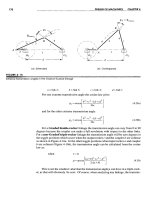
There is a closed-form solution for the roots of a cubic function
t
which allows us to
associated with the
calculate in advance that the roots of this particular cubic are all real and are x
=
-7.562,
eliminant of all but one
variable must be solved by
-1.777, and 6.740.
iteration. However, if
Figure 4-18 shows this function plotted over a range of x.
In
Figure 4-18a, an initial
factoring of the polynomial
guess value of Xl
=
1.8 is chosen. Newton's algorithm evaluates the function for this
into terms of degree four or
guess value, finding YI. The value of YI is compared to a user-selected tolerance (say
less is possible, all roots

may be found without
0.001) to see if it is close enough to zero to call Xl the root. If not, then the slope (m) of
iteration. Therefore the
the function at Xl, YI is calculated either by using an analytic expression for the deriva-
only truly symbolic
tive of the function or by doing a numerical differentiation (less desirable). The equa-
solutions are those that can
tion of the tangent line is then evaluated to find its intercept at
X2
which is used as a new
be factored into terms of
guess value. The above process is repeated, finding
Y2;
testing it against the user select-
fourth degree or less. This
ed tolerance; and, if it is too large, calculating another tangent line whose
X
intercept is
is the formal definition of a
closed form solution."
used as a new guess value. This process is repeated until the value of the function
Yi
at
the latest
Xi
is close enough to zero to satisfy the user.
t
Viete's method from "De
The Newton's algorithm described above can be expressed algebraically (in
Emendatione" by Francois

pseudocode) as shown in equation 4.35. The function for which the roots are sought is
Viete (1615) as described
fix), and its derivative is
f
(x). The slope m of the tangent line is equal to
f
(x) at the cur-
in reference [4].
rent point
Xi Yi.
If the initial guess value is close to a root, this algorithm will converge rapidly to the
solution. However, it is quite sensitive to the initial guess value. Figure 4-18b shows
the result of a slight change in the initial guess from Xl
=
1.8 to Xl
=
2.5. With this slight-
ly different guess it converges to another root. Note also that if we choose an initial guess
of Xl
=
3.579 which corresponds to a local maximum of this function, the tangent line
will be horizontal and will not intersect the
X
axis at all. The method fails in this situa-
tion. Can you suggest a value of Xl that would cause it to converge to the root at X
=
6.74?
So this method has its drawbacks. It may fail to converge.
It
may behave chaotical-

ly.
*
It
is sensitive to the guess value. It also is incapable of distinguishing between mul-
tiple circuits in a linkage. The circuit solution it finds is dependent on the initial guess.
It requires that the function be differentiable, and the derivative as well as the function
must be evaluated at every step. Nevertheless, it is the method of choice for functions
whose derivatives can be efficiently evaluated and which are continuous in the region of
the root. Furthermore, it is about the only choice for systems of nonlinear equations.
* Kramer[3] points out that
"the Newton Raphson
algorithm can exhibit
chaotic behavior when
there are multiple solutions
to kinematic constraint
equations Newton
Raphson has no mechanism
for distinguishing between
the two solutions"
(circuits). He does an
experiment with just two
links, exactly analogous to
finding the angles of the
coupler and rocker in the
fourbar linkage position
problem, and finds that the
initial guess values need to
be quite close to the
desired solution (one of the
two possible circuits) to

avoid divergence or chaotic
oscillation between the two
solutions.
Equation Solvers
Some commercially available equation solver software packages include the ability to
do a Newton-Raphson iterative solution on sets of nonlinear simultaneous equations.
TKSolver* and Mathcaat are examples. TKSolver automatically invokes its Newton-
Raphson solver when it cannot directly solve the presented equation set, provided that
enough guess values have been supplied for the unknowns. These equation solver tools
are quite convenient in that the user need only supply the equations for the system in
"raw" form such as equation 4.4la. It is not necessary to arrange them into the Newton-
Raphson algorithm as shown in the previous section. Lacking such a commercial equa-
tion solver, you will have to write your own computer code to program the solution as
described above. Reference [5] is a useful aid in this regard. The CD-ROM included
with this text contains example TKSolver files for the solution of this fourbar position
problem as well as others.
4.14
REFERENCES
1
Waldron, K. J., and S.V.Sreenivasan. (1996). "A Studyof the Solvabilityof the PositionProblem
for Multi-CircuitMechanismsby Wayof Exampleof the DoubleButterflyLinkage."Journal of
Mechanical Design, 118(3), p. 390.
2
Chase, T.R., and J. A. Mirth. (1993). "Circuitsand BranchesofSingle-Degree-of-FreedomPlanar
Linkages."Journal of Mechanical Design, 115, p. 223.
3
Kramer, G. (1992). Solving Geometric Constraint Systems: A Case Study in Kinematics. MIT
Press:Cambridge,pp. 155-158.

4
Press, W.H., et aI. (1986). Numerical Recipes: The Art of Scientific Computing. Cambridge
UniversityPress:Cambridge,pp. 145-146.
5
Ibid,pp. 254-273.
4.15
PROBLEMS
4-1 A position vector is defined as having a length equal to your height in inches (or
centimeters). The tangent of its angle is defined as your weight in pounds (or
kilograms) divided by your age in years. Calculate the data for this vector and:
a. Draw the position vector to scale on cartesian axes.
b. Write an expression for the position vector using unit vector notation.
c.
Write an expression for the position vector using complex number notation, in both
polar and cartesian fonns.
4-2
A particle is traveling along an arc of 6.5-in radius. The arc center is at the origin of a
coordinate system. When the particle is at position A, its position vector makes a 45°
angle with the X axis. At position B, its vector makes a 75° angle with the X axis.
*
Universal Technical
Draw this system to some convenient scale and:
Systems, 1220 Rock St.
a.
Write an expression for the particle's position vector in position A using complex
Rockford, IL 61101, USA.
number notation, in both polar and cartesian fonns.
(800) 435-7887
b. Write an expression for the particle's position vector in position B using complex
number notation, in both polar and cartesian fonns.

t Mathsoft, 201 Broadway,
c.
Write a vector equation for the position difference between points Band A. Sub-
Cambridge, MA 02139
stitute the complex number notation for the vectors in this equation and solve for
(800) 628-4223
the position difference numerically.
d.
Check the result of part c with a graphical method.
188
5.0
INTRODUCTION
With the fundamentals of position analysis established, we can now use these techniques
to synthesize linkages for specified output positions analytically. The synthesis tech-
niques presented in Chapter 3 were strictly graphical and somewhat intuitive. The ana-
lytical synthesis procedure is algebraic rather than graphical and is less intuitive. How-
ever, its algebraic nature makes it quite suitable for computerization. These analytical
synthesis methods were originated by Sandor[1] and further developed by his students,
Erdman,[2] Kaufman,[3] and Loerch et aI.l4,S]
5.1
TYPESOF KINEMATIC SYNTHESIS

Erdman and Sandor[6] define three types of kinematic synthesis, function, path, and
motion generation, which were discussed in Section 3.2. Brief definitions are repeated
here for your convenience.
FUNCTION GENERATION is defined as the correlation of an input function with
an output function in a mechanism. Typically, a double-rocker or crank-rocker is the
result, with pure rotation input and pure rotation output. A slider-crank linkage can be a
function generator as well, driven from either end, i.e., rotation in and translation out or
vice versa.
PATH GENERATION is defined as the control of a point in the plane such that it
follows some prescribed path. This is typically accomplished with a fourbar crank-rock-
e~or double-rocker, wherein a point on the coupler traces the desired output path. No
attempt is made in path generation to control the orientation of the link which contains
the point of interest. The coupler curve is made to pass through a set of desired output
points. However, it is common for the timing of the arrival of the coupler point at partic-
ular locations along the path to be defined. This case is called path generation with pre-
scribed timing and is analogous to function generation in that a particular output func-
tion is specified.
MOTION GENERATION
is defined as the control of a line in the plane such that it
assumes some sequential set of prescribed positions. Here orientation of the link con-
taining the line is important. This is typically accomplished with a fourbar crank-rocker
or double-rocker, wherein a point on the coupler traces the desired output path and the
linkage also controls the angular orientation of the coupler link containing the output line
of interest.
5.2 PRECISION POINTS
The points, or positions, prescribed for successive locations of the output (coupler or
rocker) link in the plane are generally referred to as precision points or precision posi-
tions. The number of precision points which can be synthesized is limited by the num-
ber of equations available for solution. The fourbar linkage can be synthesized by
closed-form methods for up to five precision points for motion or path generation with

prescribed timing (coupler output) and up to seven points for function generation (rock-
er output). Synthesis for two or three precision points is relatively straightforward, and
each of these cases can be reduced to a system of linear simultaneous equations easily
solved on a calculator. The four or more position synthesis problems involve the solu-
tion of nonlinear, simultaneous equation systems, and so are more complicated to solve,
requiring a computer.
Note that these analytical synthesis procedures provide a solution which will be able
to "be at" the specified precision points, but no guarantee is provided regarding the link-
age's behavior between those precision points. It is possible that the resulting linkage
will be incapable of moving from one precision point to another due to the presence of a
toggle position or other constraint. This situation is actually no different than that of the
graphical synthesis cases in Chapter 3, wherein there was also the possibility of a toggle
position between design points. In fact, these analytical synthesis methods are just an
alternate way to solve the same multi position synthesis problems. One should still build
a simple cardboard model of the synthesized linkage to observe its behavior and check
for the presence of problems, even if the synthesis was performed by an esoteric analyt-
ical method.
5.3 TWO-POSITION MOTION GENERATION BY ANALYTICAL
SYNTHESIS
Figure 5-1 shows a fourbar linkage in one position with a coupler point located at a first
precision position Pl' It also indicates a second precision position (point Pz) to be
achieved by the rotation of the input rocker, link 2, through an as yet unspecified angle
~z.
Note also that the angle of the coupler link 3 at each of the precision positions is
defined by the angles of the position vectors Zl and Zz. The angle
<I>
corresponds to the