DESIGN OF MACHINERYAN INTRODUCTION TO THE SYNTHESIS AND ANALYSIS OF MECHANISMS AND MACHINES phần 4 pptx

from
Ir,3.
You can see that the wheel center has a significant horizontal component of
motion as it moves up over the bump. This horizontal component causes the wheel cen-
ter on that side of the car to move forward while it moves upward, thus turning the axle
(about a vertical axis) and steering the car with the rear wheels in the same way that you
steer a toy wagon. Viewing the path of the instant center over some range of motion
gives a clear picture of the behavior of the coupler link. The undesirable behavior of this
suspension linkage system could have been predicted from this simple instant center
analysis before ever building the mechanism.
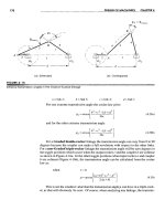
Another practical example of the effective use of instant centers in linkage design is
shown in Figure 6-13, which is an optical adjusting mechanism used to position a mirror
and allow a small amount of rotational adjustment.
[1]
A more detailed account of this
design case study
[2]
is provided in Chapter 18. The designer, K. Towfigh, recognized
that
Ir,3
at point
E
is an instantaneous "fixed pivot" and will allow very small pure rota-
tions about that point with very small translational error. He then designed a one-piece,
plastic fourbar linkage whose "pin joints" are thin webs of plastic which flex to allow
slight rotation. This is termed a compliant linkage, one that uses elastic deformations
of the links as hinges instead of pin joints. He then placed the mirror on the coupler at
11,3. Even the fixed link 1 is the same piece as the "movable links" and has a small set
screw to provide the adjustment. A simple and elegant design.
6.5 CENTRODES
Figure 6-14 illustrates the fact that the successive positions of an instant center (or cen-

tro) form a path of their own. This path, or locus, of the instant center is called the cen-
trode. Since there are two links needed to create an instant center, there will be two cen-
trodes associated with anyone instant center. These are formed by projecting the path
of the instant center first on one link and then on the other. Figure 6-14a shows the locus
of instant center
Ir,3
as projected onto link 1. Because link I is stationary, or fixed, this
is called the fixed centrode. By temporarily inverting the mechanism and fixing link 3
as the ground link, as shown in Figure 6-14b, we can move link 1 as the coupler and
project the locus of 11,3 onto link 3. In the original linkage, link 3 was the moving cou-
pler, so this is called the moving centrode. Figure 6-l4c shows the original linkage with
both fixed and moving centrodes superposed.
The definition of the instant center says that both links have the same velocity at that
point, at that instant. Link 1 has zero velocity everywhere, as does the fixed centrode.
So, as the linkage moves, the moving centrode must roll against the fixed centrode with-
out slipping. If you cut the fixed and moving centrodes out of metal, as shown in Figure
6-14d, and roll the moving centrode (which is link 3) against the fixed centrode (which
is link 1), the complex motion of link 3 will be identical to that of the original linkage.
All of the coupler curves of points on link
3
will have the same path shapes as in the orig-
inallinkage. We now have, in effect, a "linkless" fourbar linkage, really one composed
of two bodies which have these centrode shapes rolling against one another. Links 2 and
4 have been eliminated. Note that the example shown in Figure 6-14 is a non-Grashof
fourbar. The lengths of its centrodes are limited by the double-rocker toggle positions.
All instant centers of a linkage will have centrodes. If the links are directly connect-
ed by a joint, such as lz,3, 13,4, h,2, and 1
1
,4, their fixed and moving centrodes will de-

generate to a point at that location on each link. The most interesting centrodes are those
involving links not directly connected to one another such as
1
1
,3
and
h,4.
If we look at
the double-crank linkage in Figure 6-l5a in which links 2 and 4 both revolve fully, we
see that the centrodes of 11,3 form closed curves. The motion of link 3 with respect to
link 1 could be duplicated by causing these two centrodes to roll against one another
without slipping. Note that there are two loops to the moving centrode. Both must roll
on the single-loop fixed centrode to complete the motion of the equivalent double-crank
linkage.
We have so far dealt largely with the instant center 11,3. Instant center lz,4 involves
two links which are each in pure rotation and not directly connected to one another. If
we use a special-case Grashoflinkage with the links crossed (sometimes called an anti-
parallelogram linkage), the centrodes of lz,4 become ellipses as shown in Figure 6-l5b.
To guarantee no slip, it will probably be necessary to put meshing teeth on each centrode.
We then will have a pair of elliptical, noncircular gears, or gearset, which gives the
same output motion as the original double-crank linkage and will have the same varia-
tions in the angular velocity ratio and mechanical advantage as the linkage had. Thus
we can see that gearsets are also just fourbar linkages in disguise. Noncircular gears
find much use in machinery, such as printing presses, where rollers must be speeded and
slowed with some pattern during each cycle or revolution. More complicated shapes of
noncircular gears are analogous to cams and followers in that the equivalent fourbar link-
age must have variable-length links. Circular gears are just a special case of noncircu-
lar gears which give a constant angular velocity ratio and are widely used in all ma-
chines. Gears and gearsets will be dealt with in more detail in Chapter 10.
In general, centrodes of crank-rockers and double- or triple-rockers will be open

curves with asymptotes. Centrodes of double-crank linkages will be closed curves. Pro-
gram FOURBARwill calculate and draw the fixed and moving centrodes for any linkage
input to it. Input the datafiles F06-l4.4br, F06-15aAbr, and F06-l5bAbr into program
FOURBARto see the centrodes of these linkage drawn as the linkages rotate.
A "linkless" linkage
A common example of a mechanism made of centrodes is shown in Figure 6-16a. You
have probably rocked in a Boston or Hitchcock rocking chair and experienced the sooth-
ing motions that it delivers to your body. You may have also rocked in a platfonn rocker
as shown in Figure 6-16b and noticed that its motion did not feel as soothing.
There are good kinematic reasons for the difference. The platform rocker has a fixed
pin joint between the seat and the base (floor). Thus all parts of your body are in pure
rotation along concentric arcs. You are in effect riding on the rocker of a linkage.
The Boston rocker has a shaped (curved) base, or "runners," which rolls against the
floor. These runners are usually not circular arcs. They have a higher-order curve con-
tour. They are, in fact, moving centrodes. The floor is the fixed centrode. When one
is rolled against the other, the chair and its occupant experience coupler curve motion.
Every part of your body travels along a different sixth-order coupler curve which pro-
vides smooth accelerations and velocities and feels better than the cruder second-order
(circular) motion of the platform rocker. Our ancestors, who carved these rocking chairs,
probably had never heard of fourbar linkages and centrodes, but they knew intuitively
how to create comfortable motions.
CUSpS
Another example of a centrode which you probably use frequently is the path of the tire
on your car or bicycle. As your tire rolls against the road without slipping, the road be-
comes a fixed centrode and the circumference of the tire is the moving centrode. The
tire is, in effect, the coupler of a linkless fourbar linkage. All points on the contact sur-
face of the tire move along cycloidal coupler curves and pass through a cusp of zero
velocity when they reach the fixed centrode at the road surface as shown in Figure 6-17 a.
All other points on the tire and wheel assembly travel along coupler curves which do not
have cusps. This last fact is a clue to a means to identify coupler points which will have

cusps in their coupler curve. If a coupler point is chosen to be on the moving centrode at
one extreme of its path motion (i.e., at one of the positions ofh,3), then it will have a cusp
in its coupler curve. Figure 6-17b shows a coupler curve of such a point, drawn with
program FOURBAR. The right end of the coupler path touches the moving centrode and
as a result has a cusp at that point. So, if you desire a cusp in your coupler motion, many
are available. Simply choose a coupler point on the moving centrode of link 3. Read the
diskfile F06-17bAbr into program FOURBARto animate that linkage with its coupler
curve or centrodes. Note in Figure 6-14 (p. 264) that choosing any location of instant
center Il,3 on the coupler as the coupler point will provide a cusp at that point.
6.6 VELOCITY OF SLIP
When there is a sliding joint between two links and neither one is the ground link, the
velocity analysis is more complicated. Figure 6-18 shows an inversion of the fourbar
slider-crank mechanism in which the sliding joint is floating, i.e., not grounded. To solve
for the velocity at the sliding joint
A,
we have to recognize that there is more than one
point A at that joint. There is a point A as part of link 2 (Az), a point A as part oflink 3
(A3), and a point A as part of link 4 (A
4
). This is a CASE2 situation in which we have at
least two points belonging to different links but occupying the same location at a given
instant. Thus, the relative velocity equation 6.6 (p. 243) will apply. We can usually
solve for the velocity of at least one of these points directly from the known input infor-
mation using equation 6.7 (p. 244). It and equation 6.6 are all that are needed to solve for
everything else. In this example link 2 is the driver, and
8z
and
OOz
are given for the
"freeze frame" position shown. We wish to solve for

004,
the angular velocity of link 4,
and also for the velocity of slip at the joint labeled A.
In Figure 6-18 the axis of slip is shown to be tangent to the slider motion and is the
line along which all sliding occurs between links 3 and 4. The axis of transmission is
defined to be perpendicular to the axis of slip and pass through the slider joint at A. This
axis of transmission is the only line along which we can transmit motion or force across
the slider joint, except for friction. We will assume friction to be negligible in this ex-
ample. Any force or velocity vector applied to point A can be resolved into two compo-
nents along these two axes which provide a translating and rotating, local coordinate
system for analysis at the joint. The component along the axis of transmission will do
useful work at the joint. But, the component along the axis of slip does no work, except
friction work.