DESIGN OF MACHINERYAN INTRODUCTION TO THE SYNTHESIS AND ANALYSIS OF MECHANISMS AND MACHINES phần 8 ppsx

14.0
INTRODUCTION
The previous chapter discussed the design of the slider-crank mechanism as used in the
single-cylinder internal combustion engine and piston pumps. We will now extend the
design to multicylinder configurations. Some of the problems with shaking forces and
torques can be alleviated by proper combination of multiple slider-crank linkages on a
common crankshaft. Program ENGINE, included with this text, will calculate the equa-
tions derived in this chapter and allow the student to exercise many variations of an en-
gine design in a short time. Some examples are provided as disk files to be read into the
program. These are noted in the text. The student is encouraged to investigate these ex-
amples with program ENGINE in order to develop an understanding of and insight to the
subtleties of this topic. A user manual for program ENGINE is provided in Appendix A
which can be read or referred to out of sequence, with no loss in continuity, in order to
gain familiarity with the program's operation.
As with the single-cylinder case, we will not address the thermodynamic aspects of
the internal combustion engine beyond the definition of the combustion forces necessary
to drive the device presented in the previous chapter. We will concentrate on the engine's
kinematic and mechanical dynamics aspects. It is not our intention to make an "engine
designer" of the student so much as to apply dynamic principles to a realistic design
problem of general interest and also to convey the complexity and fascination involved
in the design of a more complicated dynamic device than the single-cylinder engine.
639
14.1 MUlTICYLINDER ENGINE DESIGNS
Multicylinder engines are designed in a wide variety of configurations from the simple
inline arrangement to vee, opposed, and radial arrangements some of which are shown
in Figure 14-1. These arrangements may use any of the stroke cycles discussed in Chap-
ter 13, Clerk, Otto, or Diesel.

INLINE ENGINES The most common and simplest arrangement is an inline engine
with its cylinders all in a common plane as shown in Figure 14-2. Two-,* three-,* four,
five, and six-cylinder inUne engines are in common use. Each cylinder will have its in-
dividual slider-crank mechanism consisting of a crank, conrad, and piston. The cranks
are formed together in a common crankshaft as shown in Figure 14-3. Each cylinder's
crank on the crankshaft is referred to as a crank throw. These crank throws will be ar-
ranged with some phase angle relationship one to the other, in order to stagger the mo-
tions of the pistons in time. It should be apparent from the discussion of shaking forces
and balancing in the previous chapter that we would like to have pistons moving in op-
posite directions to one another at the same time in order to cancel the reciprocating in-
ertial forces. The optimum phase angle relationships between the crank throws will dif-
fer depending on the number of cylinders and the stroke cycle of the engine. There will
usually be one (or a small number at) viable crank throw arrangements for a given en-
gine configuration to accomplish this goal. The engine in Figure 14-2 is a four-stroke
cycle, four-cylinder, inline engine with its crank throws at 0, 180, 180, and 0° phase
angles which we will soon see are optimum for this engine. Figure 14-3 shows the crank-
shaft, connecting rods and pistons for the same design of engine as in Figure 14-2.
VEE ENGINES
in two-,
*
four-,
*
six-, eight-, ten-,
t
and twelve-cylinder+ versions
are produced, with vee six and vee eight being the most common configurations. Figure
14-4 shows a cross section and Figure 14-5 a cutaway of a 60° vee -twelve engine.
Vee
engines

can be thought of as two inline engines grafted together onto a common crank-
shaft. The two "inline" portions, or
banks,
are arranged with some
vee angle
between
them. Figure 14-ld shows a vee-eight engine. Its crank throws are at 0,90,270, and
180° respectively. A vee eight's vee angle is 90°. The geometric arrangements of the
crankshaft (phase angles) and cylinders (vee angle) have a significant effect on the dy-
namic condition of the engine. We will soon explore these relationships in detail.
OPPOSED ENGINES
are essentially vee engines with a vee angle of 180°. The pis-
tons in each bank are on opposite sides of the crankshaft as shown in Figure 14-6. This
arrangement promotes cancellation of inertial forces and is popular in aircraft engines.
§
It has also been used in some automotive applications.
II
RADIAL ENGINES
have their cylinders arranged radially around the crankshaft in
nearly a common plane. These were common on World War II vintage aircraft as they
allowed large displacements, and thus high power, in a compact form whose shape was
well suited to that of an airplane. Typically air cooled, the cylinder arrangement allowed
good exposure of all cylinders to the airstream. Large versions had multiple rows of ra-
dial cylinders, rotationally staggered to allow cooling air to reach the back rows. The
gas turbine jet engine has rendered these radial aircraft engines obsolete.
ROTARY ENGINES
were an interesting variant on the aircraft radial engine. Sim-
ilar in appearance and cylinder arrangement to the radial engine, the anomaly was that
the crankshaft was the stationary ground plane. The propeller was attached to the crank-
case (block) which rotated around the crankshaft! It is a kinematic inversion of the radi-

al engine. At least it didn't need a flywheel.
Many other configurations of engines have been tried over the century of develop-
ment of this ubiquitous device. The bibliography at the end of this chapter contains sev-
eral references which describe other engine designs, the usual, unusual, and exotic. We
will begin our detailed exploration of multicylinder engine design with the simplest con-
figuration, the inline engine, and then progress to the vee and opposed versions.
We must establish some convention for the measurement of these phase angles
which will be:
1 The first (front) cylinder will be number 1 and its phase angle will always be zero.
It is the reference cylinder for all others.
2 The phase angles of all other cylinders will be measured with respect to the crank
throw for cylinder 1.
3 Phase angles are measured internal to the crankshaft, that is, with respect to a rotat-
ing coordinate system embedded in the first crank throw.
4 Cylinders will be numbered consecutively from front to back of the engine.
The phase angles are defined in a crank phase diagram as shown in Figure 14-7
for a four-cylinder, inline engine. Figure l4-7a shows the crankshaft with the throws
numbered clockwise around the axis. The shaft is rotating counterclockwise. The pis-
tons are oscillating horizontally in this diagram, along the x axis. Cylinder 1 is shown
with its piston at top dead center (TDC). Taking that position as the starting point for the
abscissas (thus time zero) in Figure 14-7b, we plot the velocity of each piston for two
revolutions of the crank (to accommodate one complete four-stroke cycle). Piston 2 ar-
rives at TDC 90° after piston 1 has left. Thus we say that cylinder 2 lags cylinder 1 by
90 degrees. By convention a lagging event is defined as having a negative phase angle,
shown by the clockwise numbering of the crank throws. The velocity plots clearly show
that each cylinder arrives at TDC (zero velocity) 90° later than the one before it. Nega-
tive velocity on the plots in Figure l4-7b indicates piston motion to the left (down stroke)
in Figure l4-7a; positive velocity indicates motion to the right (up stroke).
For the discussion in this chapter we will assume counterclockwise rotation of all
crankshafts, and all phase angles will thus be negative. We will, however, omit the neg-

ative signs on the listings of phase angles with the understanding that they follow this
convention.
Figure 14-7 shows the timing of events in the cycle and is a necessary and useful
aid in defining our crankshaft design. However, it is not necessary to go to the trouble of
drawing the correct sinusoidal shapes of the velocity plots to obtain the needed informa-
tion. All that is needed is a schematic indication of the relative positions within the cy-
11.11
CONTROLLING INPUTTORQUE-flYWHEElS
The typically large variation in accelerations within a mechanism can cause significant
oscillations in the torque required to drive it at a constant or near constant speed. The
peak torques needed may be so high as to require an overly large motor to deliver them.
However, the average torque over the cycle, due mainly to losses and external work done,
may often be much smaller than the peak torque. We would like to provide some means
to smooth out these oscillations in torque during the cycle. This will allow us to size the
motor to deliver the average torque rather than the peak torque. One convenient and rel-
atively inexpensive means to this end is the addition of a flywheel to the system.
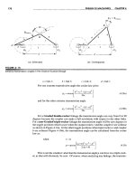
TORQUE VARIATION
Figure 11-8 shows the variation in the input torque for a
crank-rocker fourbar linkage over one full revolution of the drive crank. It is running at
a constant angular velocity of 50 rad/sec. The torque varies a great deal within one cy-
cle of the mechanism, going from a positive peak of 341.7 Ib-in to a negative peak of
-166.41b-in. The average value of this torque over the cycle is only 70.21b-in, being
due to the external work done plus losses. This linkage has only a 12-lb external force
applied to link 3 at the CG and a 25 Ib-in external torque applied to link 4. These small
external loads cannot account for the large variation in input torque required to maintain
constant crank speed. What then is the explanation? The large variations in torque are
evidence of the kinetic energy that is stored in the links as they move. We can think of

the positive pulses of torque as representing energy delivered by the driver (motor) and
stored temporarily in the moving links, and the negative pulses of torque as energy at-
tempting to return from the links to the driver. Unfortunately most motors are designed
to deliver energy but not to take it back. Thus the "returned energy" has no place to go.
Figure 11-9 shows the speed torque characteristic of a permanent magnet (PM) DC
electric motor. Other types of motors will have differently shaped functions that relate
motor speed to torque as shown in Figure 2-32 and 2-33 (pp. 62-63), but all drivers
average, the sum of positive area above an average line is equal to the sum of negative area
below that line.) The integration limits in equation 11.18 are from the shaft angle 8 at which
the shaft (j)is a minimum to the shaft angle 8 at which (j)is a maximum.
3
The minimum (j)will occur after the maximum positive energy has been delivered from the
motor to the load, i.e., at a point (8) where the summation of positive energy (area) in the
torque pulses is at its largest positive value.
4
The maximum (j)will occur after the maximum negative energy has been returned to the load,
i.e., at a point (8) where the summation of energy (area) in the torque pulses is at its largest
negative value.
5
To find these locations in 8 corresponding to the maximum and minimum (j)'s and thus find
the amount of energy needed to be stored in the flywheel, we need to numerically integrate
each pulse of this function from crossover to crossover with the average line. The crossover
points in Figure 11-11 have been labeled A, B, C, and D. (Program FOURBARdoes this inte-
gration for you numerically, using a trapezoidal rule.)
6
The FOURBARprogram prints the table of areas shown in Figure 11-11. The positive and
negative pulses are separately integrated as described above. Reference to the plot of the

torque function will indicate whether a positive or negative pulse is the first encountered in
a particular case. The first pulse in this example is a positive one.
7
The remaining task is to accumulate these pulse areas beginning at an arbitrary crossover (in
this case point A) and proceeding pulse by pulse across the cycle. Table 11-1 shows this pro-
cess and the result.
8
Note in Table 11-1 that the minimum shaft speed occurs after the largest accumulated posi-
tive energy pulse (+200.73 in-lb) has been delivered from the driveshaft to the system. This
delivery of energy slows the motor down. The maximum shaft speed occurs after the largest
accumulated negative energy pulse (-60.32 in-lb) has been received back from the system
by the driveshaft. This return of stored energy will speed up the motor. The total energy
variation is the algebraic difference between these two extreme values, which in this exam-
ple is -261.05 in-lb. This negative energy coming out of the system needs to be absorbed by
the flywheel and then returned to the system during each cycle to smooth the variations in
shaft speed.
the torque curve (see Table 11-1, p. 552) and the average shaft
(i)
to compute the needed
system
Is.
The physical flywheel's mass moment of inertia
If
is then set equal to the re-
quired system
Is.
But if the moments of inertia of the other rotating elements on the same
driveshaft (such as the motor) are known, the physical flywheel's required
If

can be re-
duced by those amounts.
The most efficient flywheel design in terms of maximizing
Iffor
minimum material
used is one in which the mass is concentrated in its rim and its hub is supported on
spokes, like a carriage wheel. This puts the majority of the mass at the largest radius
possible and minimizes the weight for a given
If
Even if a flat, solid circular disk fly-
wheel design is chosen, either for simplicity of manufacture or to obtain a flat surface
for other functions (such as an automobile clutch), the design should be done with an eye
to reducing weight and thus cost. Since in general,
I
=
m,.2,
a thin disk of large diame-
ter will need fewer pounds of material to obtain a given
I
than will a thicker disk of small-
er diameter. Dense materials such as cast iron and steel are the obvious choices for a fly-
wheel. Aluminum is seldom used. Though many metals (lead, gold, silver, platinum) are
more dense than iron and steel, one can seldom get the accounting department's approv-
al to use them in a flywheel.
Figure 11-12 shows the change in the input torque T
1
2 for the linkage in Figure 11-8
after the addition of a flywheel sized to provide a coefficient of fluctuation of 0.05. The
oscillation in torque about the unchanged average value is now 5%, much less than what
it was without the flywheel. A much smaller horsepower motor can now be used because

the flywheel is available to absorb the energy returned from the linkage during its cycle.
11.12
A LINKAGE FORCE TRANSMISSION INDEX
The transmission angle was introduced in Chapter 2 and used in subsequent chapters as
an index of merit to predict the kinematic behavior of a linkage. A too-small transmis-
sion angle predicts problems with motion and force transmission in a fourbar linkage.
Unfortunately, the transmission angle has limited application. It is only useful for four-
bar linkages and then only when the input and output torques are applied to links that are
pivoted to ground (i.e., the crank and rocker). When external forces are applied to the
coupler link, the transmission angle tells nothing about the linkage's behavior.
Holte and Chase
[1]
define a joint-force index
(IPl)
which is useful as an indicator
of any linkage's ability to smoothly transmit energy regardless of where the loads are
applied on the linkage. It is applicable to higher-order linkages as well as to the fourbar
linkage. The IPI at any instantaneous position is defined as the ratio of the maximum
static force in any joint of the mechanism to the applied external load. If the external
load is a force, then it is:
The F
ij
are calculated from a static force analysis of the linkage. Dynamic forces
can be much greater than static forces if speeds are high. However, if this static force
transmission index indicates a problem in the absence of any dynamic forces, then the
situation will obviously be worse at speed. The largest joint force at each position is used
rather than a composite or average value on the assumption that high friction in anyone
joint is sufficient to hamper linkage performance regardless of the forces at other joints.
Equation 11.23a is dimensionless and so can be used to compare linkages of differ-
ent design and geometry. Equation 11.23b has dimensions of reciprocal length, so cau-

tion must be exercised when comparing designs when the external load is a torque. Then
the units used in any comparison must be the same, and the compared linkages should
be similar in size.
Equations 11.23 apply to anyone instantaneous position of the linkage. As with the
transmission angle, this index must be evaluated for all positions of the linkage over its
expected range of motion and the largest value of that set found. The peak force may
move from pin to pin as the linkage rotates. If the external loads vary with linkage posi-
tion, they can be accounted for in the calculation.
Holte and Chase suggest that the IPI be kept below a value of about 2 for linkages
whose output is a force. Larger values may be tolerable especially if the joints are de-
signed with good bearings that are able to handle the higher loads.
There are some linkage positions in which the IPI can become infinite or indetermi-
nate as when the linkage reaches an immovable position, defined as the input link or in-
put joint being inactive. This is equivalent to a stationary configuration as described in
earlier chapters provided that the input joint is inactive in the particular stationary con-
figuration. These positions need to be identified and avoided in any event, independent
of the determination of any index of merit. In some cases the mechanism may be im-
movable but still capable of supporting a load. See reference [1] for more detailed infor-
mation on these special cases.
11.13 PRACTICAL CONSIDERATIONS
This chapter has presented some approaches to the computation of dynamic forces in
moving machinery. The newtonian approach gives the most information and is neces-
sary in order to obtain the forces at all pin joints so that stress analyses of the members
can be done. Its application is really quite straightforward, requiring only the creation
of correct free-body diagrams for each member and the application of the two simple
vector equations which express Newton's second law to each free-body. Once these
equations are expanded for each member in the system and placed in standard matrix
form, their solution (with a computer) is a trivial task.
The real work in designing these mechanisms comes in the determination of the
shapes and sizes of the members. In addition to the kinematic data, the force computa-

tion requires only the masses, CG locations, and mass moments of inertia versus those
CGs for its completion. These three geometric parameters completely characterize the
member for dynamic modelling purposes. Even if the link shapes and materials are com-
pletely defined at the outset of the force analysis process (as with the redesign of an ex-
isting system), it is a tedious exercise to calculate the dynamic properties of complicated
shapes. Current solids modelling CAD systems make this step easy by computing these
parameters automatically for any part designed within them.
If, however, you are starting from scratch with your design, the blank-paper syn-
drome will inevitably rear its ugly head. A first approximation of link shapes and selec-
tion of materials must be made in order to create the dynamic parameters needed for a
"first pass" force analysis. A stress analysis of those parts, based on the calculated dy-
namic forces, will invariably find problems that require changes to the part shapes, thus
requiring recalculation of the dynamic properties and recomputation of the dynamic forc-
es and stresses. This process will have to be repeated in circular fashion (iteration-see
Chapter 1, p. 8) until an acceptable design is reached. The advantages of using a com-
puter to do these repetitive calculations is obvious and cannot be overstressed. An equa-
tion solver program such as TKSolver or Mathcad will be a useful aid in this process by
reducing the amount of computer programming necessary.
Students with no design experience are often not sure how to approach this process
of designing parts for dynamic applications. The following suggestions are offered to
get you started. As you gain experience, you will develop your own approach.
It is often useful to create complex shapes from a combination of simple shapes, at
least for first approximation dynamic models. For example, a link could be considered
to be made up of a hollow cylinder at each pivot end, connected by a rectangular prism
along the line of centers. It is easy to calculate the dynamic parameters for each of these
simple shapes and then combine them. The steps would be as follows (repeated for each
link):
1 Calculate the volume, mass, CG location, and mass moments of inertia with respect
to the local CG of each separate part of your built-up link. In our example link these
parts would be the two hollow cylinders and the rectangular prism.

2 Find the location of the composite CG of the assembly of the parts into the link by
the method shown in Section 11.4 (p. 531) and equation 11.3 (p. 524). See also Fig-
ure 11-2 (p. 526).