DESIGN OF MACHINERYAN INTRODUCTION TO THE SYNTHESIS AND ANALYSIS OF MECHANISMS AND MACHINES phần 9 docx

Note that, unlike the inertia force in equation 13.14 (p. 619), which was unaffected
by the gas force, these pin forces are a function of the gas force as well as of the
-ma
forces. Engines with larger piston diameters will experience greater pin forces as a re-
sult of the explosion pressure acting on their larger piston area.
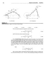
Program ENGINEcalculates the pin forces on all joints using equations 13.20 to
13.23. Figure 13-21 shows the wrist-pin force on the same unbalanced engine example
as shown in previous figures, for three engine speeds. The "bow tie" loop is the inertia
force and the "teardrop" loop is the gas force portion of the force curve. An interesting
trade-off occurs between the gas force components and the inertia force components of
the pin forces. At a low speed of 800 rpm (Figure l3-2la), the gas force dominates as
the inertia forces are negligible at small co. The peak wrist-pin force is then about 4200
lb. At high speed (6000 rpm), the inertia components dominate and the peak force is
about 4500 lb (Figure 13-2lc). But at a midrange speed (3400 rpm), the inertia force
cancels some of the gas force and the peak force is only about 3200 lb (Figure 13-2lb).
These plots show that the pin forces can be quite large even in a moderately sized (0.4
liter/cylinder) engine. The pins, links, and bearings all have to be designed to withstand
hundreds of millions of cycles of these reversing forces without failure.
Figure 13-22 shows further evidence of the interaction of the gas forces and inertia
forces on the crankpin and the wrist pin. Figures 13-22a and 13-22c show the variation
in the inertia force component on the crankpin and wrist pin, respectively, over one full
revolution of the crank as the engine speed is increased from idle to redline. Figure
13-22b and d show the variation in the total force on the same respective pins with both
the inertia and gas force components included. These two plots show only the first 90
0
of crank revolution where the gas force in a four-stroke cylinder occurs. Note that the
gas force and inertia force components counteract one another resulting in one particu-
lar speed where the total pin force is a minimum during the power stroke. This is the
same phenomenon as seen in Figure 13-21.
13.10 BALANCING THESINGLE-CYLINDER ENGINE

The derivations and figures in the preceding sections have shown that significant forces
are developed both on the pivot pins and on the ground plane due to the gas forces and
the inertia and shaking forces. Balancing will not have any effect on the gas forces,
which are internal, but it can have a dramatic effect on the inertia and shaking forces.
The main pin force can be reduced, but the crankpin and wrist pin forces will be unaf-
fected by any crankshaft balancing done. Figure 13-13 (p. 620) shows the unbalanced
shaking force as felt on the ground plane of our OA-liter-per-cylinder example engine
from program ENGINE. It is about 9700 Ib even at the moderate speed of 3400 rpm. At
6000 rpm it increases to over 30 000 lb. The methods of Chapter 12 can be applied to this
mechanism to balance the members in pure rotation and reduce these large shaking forces.
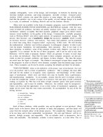
Figure 13-23a shows the dynamic model of our slider-crank with the conrod mass
lumped at both crankpin A and wrist pin B. We can consider this single-cylinder engine
to be a single-plane device, thus suitable for static balancing (see Section 13.1). It is
straightforward to statically balance the crank. We need a balance mass at some radius,
180
0
from the lumped mass at point A whose
mr
product is equal to the product of the
mass at
A
and its radius
r.
Applying equation 13.2 to this simple problem we get:
Any combination of mass and radius which gives this product, placed at 180
0
from
point A will balance the crank. For simplicity of example, we will use a balance radius
equal to r. Then a mass equal to mA placed at A ' will exactly balance the rotating mass-
es. The CG ofthe crank will then be at the fixed pivot

02
as shown in Figure 13-23a. In
a real crankshaft, actually placing the counterweight at this large a radius would not
work. The balance mass has to be kept close to the centerline to clear the piston at BDC.
Figure 13-2c shows the shape of typical crankshaft counterweights.
Figure 13-24a shows the shaking force from the same engine as in Figure 13-13 af-
ter the crank has been exactly balanced in this manner. The
Y
component of the shaking
force has been reduced to zero and the x component to about 3300 Ib at 3400 rpm. This
is a factor of three reduction over the unbalanced engine. Note that the only source of
Y
directed inertia force is the rotating mass at point
A
of Figure 13-23 (see equations 13.14,
p. 619). What remains after balancing the rotating mass is the force due to the accelera-
tion of the piston and conrod masses at point B of Figure 13-23 which are in linear trans-
lation along the X axis, as shown by the inertia force
-mBaB
at point B in that figure.
To completely eliminate this reciprocating unbalanced shaking force would require
the introduction of another reciprocating mass, which oscillates 180
0
out of phase with
the piston. Adding a second piston and cylinder, properly arranged, can accomplish this.

14.0
INTRODUCTION
The previous chapter discussed the design of the slider-crank mechanism as used in the
single-cylinder internal combustion engine and piston pumps. We will now extend the
design to multicylinder configurations. Some of the problems with shaking forces and
torques can be alleviated by proper combination of multiple slider-crank linkages on a
common crankshaft. Program ENGINE, included with this text, will calculate the equa-
tions derived in this chapter and allow the student to exercise many variations of an en-
gine design in a short time. Some examples are provided as disk files to be read into the
program. These are noted in the text. The student is encouraged to investigate these ex-
amples with program ENGINE in order to develop an understanding of and insight to the
subtleties of this topic. A user manual for program ENGINE is provided in Appendix A
which can be read or referred to out of sequence, with no loss in continuity, in order to
gain familiarity with the program's operation.
As with the single-cylinder case, we will not address the thermodynamic aspects of
the internal combustion engine beyond the definition of the combustion forces necessary
to drive the device presented in the previous chapter. We will concentrate on the engine's
kinematic and mechanical dynamics aspects. It is not our intention to make an "engine
designer" of the student so much as to apply dynamic principles to a realistic design
problem of general interest and also to convey the complexity and fascination involved
in the design of a more complicated dynamic device than the single-cylinder engine.
639
14.1 MUlTICYLINDER ENGINE DESIGNS
Multicylinder engines are designed in a wide variety of configurations from the simple
inline arrangement to vee, opposed, and radial arrangements some of which are shown
in Figure 14-1. These arrangements may use any of the stroke cycles discussed in Chap-
ter 13, Clerk, Otto, or Diesel.

INLINE ENGINES The most common and simplest arrangement is an inline engine
with its cylinders all in a common plane as shown in Figure 14-2. Two-,* three-,* four,
five, and six-cylinder inUne engines are in common use. Each cylinder will have its in-
dividual slider-crank mechanism consisting of a crank, conrad, and piston. The cranks
are formed together in a common crankshaft as shown in Figure 14-3. Each cylinder's
crank on the crankshaft is referred to as a crank throw. These crank throws will be ar-
ranged with some phase angle relationship one to the other, in order to stagger the mo-
tions of the pistons in time. It should be apparent from the discussion of shaking forces
and balancing in the previous chapter that we would like to have pistons moving in op-
posite directions to one another at the same time in order to cancel the reciprocating in-
ertial forces. The optimum phase angle relationships between the crank throws will dif-
fer depending on the number of cylinders and the stroke cycle of the engine. There will
usually be one (or a small number at) viable crank throw arrangements for a given en-
gine configuration to accomplish this goal. The engine in Figure 14-2 is a four-stroke
cycle, four-cylinder, inline engine with its crank throws at 0, 180, 180, and 0° phase
angles which we will soon see are optimum for this engine. Figure 14-3 shows the crank-
shaft, connecting rods and pistons for the same design of engine as in Figure 14-2.
VEE ENGINES
in two-,
*
four-,
*
six-, eight-, ten-,
t
and twelve-cylinder+ versions
are produced, with vee six and vee eight being the most common configurations. Figure
14-4 shows a cross section and Figure 14-5 a cutaway of a 60° vee -twelve engine.
Vee
engines

can be thought of as two inline engines grafted together onto a common crank-
shaft. The two "inline" portions, or
banks,
are arranged with some
vee angle
between
them. Figure 14-ld shows a vee-eight engine. Its crank throws are at 0,90,270, and
180° respectively. A vee eight's vee angle is 90°. The geometric arrangements of the
crankshaft (phase angles) and cylinders (vee angle) have a significant effect on the dy-
namic condition of the engine. We will soon explore these relationships in detail.
OPPOSED ENGINES
are essentially vee engines with a vee angle of 180°. The pis-
tons in each bank are on opposite sides of the crankshaft as shown in Figure 14-6. This
arrangement promotes cancellation of inertial forces and is popular in aircraft engines.
§
It has also been used in some automotive applications.
II
RADIAL ENGINES
have their cylinders arranged radially around the crankshaft in
nearly a common plane. These were common on World War II vintage aircraft as they
allowed large displacements, and thus high power, in a compact form whose shape was
well suited to that of an airplane. Typically air cooled, the cylinder arrangement allowed
good exposure of all cylinders to the airstream. Large versions had multiple rows of ra-
dial cylinders, rotationally staggered to allow cooling air to reach the back rows. The
gas turbine jet engine has rendered these radial aircraft engines obsolete.
ROTARY ENGINES
were an interesting variant on the aircraft radial engine. Sim-
ilar in appearance and cylinder arrangement to the radial engine, the anomaly was that
the crankshaft was the stationary ground plane. The propeller was attached to the crank-
case (block) which rotated around the crankshaft! It is a kinematic inversion of the radi-

al engine. At least it didn't need a flywheel.
Many other configurations of engines have been tried over the century of develop-
ment of this ubiquitous device. The bibliography at the end of this chapter contains sev-
eral references which describe other engine designs, the usual, unusual, and exotic. We
will begin our detailed exploration of multicylinder engine design with the simplest con-
figuration, the inline engine, and then progress to the vee and opposed versions.
We must establish some convention for the measurement of these phase angles
which will be:
1 The first (front) cylinder will be number 1 and its phase angle will always be zero.
It is the reference cylinder for all others.
2 The phase angles of all other cylinders will be measured with respect to the crank
throw for cylinder 1.
3 Phase angles are measured internal to the crankshaft, that is, with respect to a rotat-
ing coordinate system embedded in the first crank throw.
4 Cylinders will be numbered consecutively from front to back of the engine.
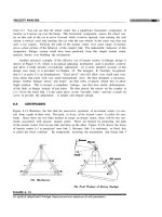
The phase angles are defined in a crank phase diagram as shown in Figure 14-7
for a four-cylinder, inline engine. Figure l4-7a shows the crankshaft with the throws
numbered clockwise around the axis. The shaft is rotating counterclockwise. The pis-
tons are oscillating horizontally in this diagram, along the x axis. Cylinder 1 is shown
with its piston at top dead center (TDC). Taking that position as the starting point for the
abscissas (thus time zero) in Figure 14-7b, we plot the velocity of each piston for two
revolutions of the crank (to accommodate one complete four-stroke cycle). Piston 2 ar-
rives at TDC 90° after piston 1 has left. Thus we say that cylinder 2 lags cylinder 1 by
90 degrees. By convention a lagging event is defined as having a negative phase angle,
shown by the clockwise numbering of the crank throws. The velocity plots clearly show
that each cylinder arrives at TDC (zero velocity) 90° later than the one before it. Nega-
tive velocity on the plots in Figure l4-7b indicates piston motion to the left (down stroke)
in Figure l4-7a; positive velocity indicates motion to the right (up stroke).
For the discussion in this chapter we will assume counterclockwise rotation of all
crankshafts, and all phase angles will thus be negative. We will, however, omit the neg-

ative signs on the listings of phase angles with the understanding that they follow this
convention.
Figure 14-7 shows the timing of events in the cycle and is a necessary and useful
aid in defining our crankshaft design. However, it is not necessary to go to the trouble of
drawing the correct sinusoidal shapes of the velocity plots to obtain the needed informa-
tion. All that is needed is a schematic indication of the relative positions within the cy-