Báo cáo khoa học: "Choosing simplified mixed models for simulations when data have a complex hierarchical organization. An example with some basic properties in Sessile oak wood (Quercus petraea Liebl.)" ppsx
Bạn đang xem bản rút gọn của tài liệu. Xem và tải ngay bản đầy đủ của tài liệu tại đây (186.14 KB, 9 trang )
G. Le Moguédec et al.Choosing simplified mixed models
Original article
Choosing simplified mixed models for simulations
when data have a complex hierarchical organization.
An example with some basic properties
in Sessile oak wood (Quercus petraea Liebl.)
Gilles Le Moguédec
*
, Jean-François Dhôte and Gérard Nepveu
LERFOB, Centre INRA de Nancy, 54280 Champenoux Cedex, France
(Received 14 February 2001; accepted 6 August 2002)
Abstract – This paper focuses on the modeling of the variability of some properties in Sessile oak wood (five swelling coefficients and wood
density). They are modeled with linear mixed models. The data have a seven-levels hierarchical organization. The variability at each level is mo-
deled with a variance matrix. Unfortunately, a model with all variances has too many parameters to be usable, so preferably only one variance
other than the residual is kept. A graphical procedure based on the comparison of residual variance in the different candidate models is used to
detect this main level. Result shows that the main level of variability is the “tree” level or the “height within tree” level for five properties. We
cannot conclude for the last property. For otherproperties,the residual variance in the model with a “tree effect” is reduced to 40% of the residual
variance of the model without structuring of variability. If the applications of models deal with the variability of properties, this “tree level” can-
not be neglected.
linear mixed model / Sessile oak / structuring of variability / “tree” effect
Résumé – Simplifier un modèle mixte destiné à effectuer des simulations lorsque les données ont une structure hiérarchique complexe.
Exemple de quelques propriétés de base du bois de Chêne sessile (Quercus petraea Liebl.). Cet article traite de la modélisation de la variabi
-
lité de propriétés du bois de Chêne sessile (cinq coefficients de gonflement et la densité du bois). Ces propriétés sont modélisées à l’aide de mo
-
dèles linéaires mixtes. Les données ont une organisation hiérarchique à sept niveaux. La variabilité à chacun de ces niveaux est modélisée par
une matrice de variance. Cependant, le modèle avec toutes les variances comprend trop de paramètres pour être utilisable, aussi le choix est fait
de ne tenir compte que d’une seule variance en plus de la variance résiduelle. On utilise une procédure graphique basée sur la comparaison des
variances résiduelles des différents modèles candidats pour détecter le niveau principal de la variabilité. Ce niveau principal est ainsi le niveau
« arbre » ou le niveau « hauteur dans l’arbre » pour cinq des propriétés. On ne peut pas conclure pour la sixième. Pour toutes les autres proprié
-
tés, la prise en compte d’un effet arbre permet de réduire la variance résiduelle à 40 % de la valeur obtenue dans un modèle sans structuration de
la variabilité. Si la variabilité des propriétés est un facteur important pour les applications des modèles, ce niveau « arbre » ne peut pas être
négligé.
modèle linéaire mixte / Chêne sessile / structuration de la variabilité / effet « arbre »
1. INTRODUCTION
Sessile and Pedunculate oaks (Quercus petraea Liebl. and
Q. robur L.) predominate in the French forest resource (32%
of the forest area is dominated by these two species). They
occur in a large range of ecological situations, from the
Atlantic coast (mild climate) to the eastern borders
(semi-continental climate), and from fresh valleys to dry
south slopes as well as on a large range of parent bedrocks
[18]. Pedunculate oak is more specialized in favourable site
conditions [3] but, due to its pioneer habit, it is commonly
present in under-optimal sites. Sessile oak has more pro
-
nounced characteristics of a social species, and can afford
Ann. For. Sci. 59 (2002) 847–855 847
© INRA, EDP Sciences, 2002
DOI: 10.1051/forest:2002083
* Correspondence and reprints
Tel.: 03 83 39 41 42; fax: 03 83 39 40 69; e-mail:
high levels of competition: therefore, it is widely tended ac
-
cording to the high forest regime. Pure, even-aged high for
-
ests of Sessile oak have been managed very precautiously for
decades, and they provide now the best quality assortments
(slow-grown trees, with long boles, “finely-grained” timber
with light colour and low density, used for veneer, barrels,
furniture). Nevertheless, the major part of the resource in
both oaks is composed of coppice-with-standards (CwS) sys
-
tems, i.e. stands inherited from past practices of coppicing,
while keeping a low number of standards (20 to 100 large
oaks per hectare). These standards differ markedly from
high-forest-grown oaks: faster growth, shorter boles, and
lower quality. Private owners, who cannot afford the very
long rotations of public forests (180 to 250 years), more and
more, favour semi-intensive management of oaks (by the
CwS system or by enhancing future crop tree growth in high
forest regimes). For these reasons, there is an increasing need
for integrated simulation models, providing detailed outputs
in terms of stand yield, tree growth and the main quality crite
-
ria, including log grading [15].
Oak-based ecosystems are also particularly important for
other functions than just yield: structuring of landscapes, spe-
cies and ecosystem conservation (associated broadleaves in
the understorey), biodiversity [19], conservation of genetic
diversity [21]. In the perspective of future climate change,
forest managers anticipate that especially Sessile oak might
play a crucial role, due to its well-known drought-tolerance.
Furthermore, recent studies have shown that the productivity
of oaks has steadily increased over the past century [4, 7]: the
possible nutritional deficiencies that might occur (especially
on poor soils) are of particular importance for forest manag-
ers and forest policy-makers.
In these multiple regards, it seems important to maintain a
sufficient degree of genetic variability in oak stands, in order
to preserve the adaptive capacities present in the natural pop
-
ulations. But this management objective, in turn, requires a
better knowledge of tree-to-tree variability, at all levels of
management: regional resource evaluation, forest planning
methods, stand silvicultural projections. In the past years, ad
-
vances in growth modeling made it possible to simulate Ses
-
sile oak stand dynamics under contrasted site-silviculture
conditions [16]. Although there is still much individual-tree
growth variation, which is not accounted for by the model, we
have thought preferable to concentrate first on the tree-to-tree
variability for wood quality features (namely wood density
and behavior of timber during drying). Indeed, previous work
by Polge and Keller [17] had shown that (i) silviculture
strongly influences the properties of oak wood (larger rings
are associated with higher density), and (ii) the density varia
-
tion between trees within a stand is very large.
In this paper we present an analysis of the structuring of
variability for some important wood characteristics of Sessile
oak: five swelling coefficients and the wood density. This
variability is a major problem to suitably model the
properties. Zhang et al. [22] showed that inter-tree variation
represents a large part of the total variation in Sessile oak, but
they did not take into account other potential sources of vari
-
ability as the applied silviculture or site growth conditions.
Therefore, we have to study the structuring of the variability
before taking it into account.
Between 1992 and 1995, an important research
programme was undertaken, withthe objectives of describing
and modeling the variability of Sessile oak growth, morphol
-
ogy and wood quality, based on appropriate sampling plans
and use of available statistical methods (mixed models). This
programme associated the Office National des Forêts (French
Forestry Office) and our research teams at INRA-
Champenoux, working in the fields of growth and yield,
silviculture and wood science. The main aspect of this Project
was the constitution and analysis of a large collection (82) of
commercial-size Sessile oaks, covering the major sources of
variability which are present in the species: regional popula
-
tions (ranging from Normandy to Alsace), site qualities (ex
-
cept on calcareous bedrocks, where the dry sites occupied by
oaks can hardly provide large diameters), silvicultural sys
-
tems (coppice-with-standards and high forest). These
82 trees were intensively described: stem analyses, mapping
of annual rings and sapwood-heartwood, measurement of
several wood quality criteria (density, swelling, colour, spiral
grain, multiseriate wood rays) on both standard small-size
samples and industrial-size boards.
Our data have a hierarchical organization. Each level of
the hierarchy could be a level of structuring of the variability.
This paper studies the decomposition of the variability
through the different levels of hierarchy. If possible, the best
model should take into account all the significant levels of
variability. But such a complex model is too complicated to
be useful for further simulations, so that only the main levels
have to be retained.
This paper studies the evolution of the variability through
the different levels of the hierarchy, in order to detect the
main level of variability to be included in a model relevant for
use in simulations, and thus to obtain a good compromise be
-
tween the heaviness and efficiency of the model.
2. MATERIALS, SAMPLING
AND MEASUREMENTS
The sample used here is a collection of 82 mature Sessile oak
trees (Quercus petraea Liebl.). It was designed in order to answer
two series of questions:
– describe and model the dynamics of stem taper and the distribu
-
tion of sapwood inside the tree; study the local effect of ramifica
-
tions; analyse the variation of these phenomenons when trees differ
by the general vigour and morphology;
– model the variability of local wood properties (density, swelling,
color, spiral grain, multiseriate wood rays) as functions of position
inside the tree (age from the pith, vertical level) and ring width.
The principles of the sampling plan were, on the one hand, to ex
-
plore a large range of growth rates and stem morphologies, on the
848 G. Le Moguédec et al.
other hand, to cover most of the sources of variability that are en
-
countered in the geographical area of the species distribution.
2.1. Tree selection
The sample is divided into 5 regions of contrasted climates: north
of Alsace (sandstone hills and sandy-loamy soils in the plain), Pla
-
teau lorrain, Val de Loire, Basse-Normandie, Allier-Bourbonnais
(Center of France). In each region, a large range of site quality was
represented. In each combination (region × site), stands belonging to
two types of structure were prospected: usual high forest, cop
-
pice-with-standards.
Site quality was determined from an inventory of ground vegeta
-
tion and the analysis of a soil core (1 m deep). The soil descriptions
(nutrient richness and water regime) were summarized in each re
-
gion and classified into 3 categories: good, medium and poor site
quality, using expert knowledge of Sessile oak autecology [3].
In each family (region-site-structure), one or two stands were se
-
lected, containing a sufficient number of oaks larger than 40 cm in
diameter. In each stand, two trees were chosen (occasionally only
one tree, especially on very poor, humid sites where the mixture
with Pedunculate oak was a problem), at distances of 30 to 200 m
from each other. The site diagnostic was done at the proximity of
preselected trees; the choice was revised until soil conditions were
reasonably similar for the 2 trees of the same stand.
For tree selection, we looked for dominant (eventually
codominant) individuals of “standard” quality, i.e. not excellent, but
representative of the population that would be kept by silviculturists
until the final harvest. Defects like leaning stems, basal curvature,
excessive grain angle, frost cracks, abundant epicormics were re-
jected.
More detailed description of the sampling can be found in [8].
2.2. Wood sample preparation and measurement
On each tree, a disk has been taken at breast height (1-height) and
another at half-height between breast height and the crown basis
(2-height) for 52 trees.
From each disk, the radius with the biggest length from the pith
to the bark and its opposite were cut (respectively called 1- and
5-stripe).
Sixteen-mm-sized cubes were cut from these stripes when
air-dried. They were cut within areas exhibiting an homogeneous
ring width and oriented according to the three orthotropic directions
of wood (longitudinal, radial and tangential). Therefore the cubes of
a same stripe are not necessarily closely related. There are nearly 8
to 12 cubes per stripe.
The first level of hierarchy in the data is based on the stand struc
-
ture: high forest or coppice with standards.
The second one is the fertility of the stands with 3 modalities,
good, medium or poor, nested in the stand structure. At this level,
there are 6 different modalities (3 fertilities × 2 structures).
The third level is the region. There are 5 regions with observa
-
tions, but not all the2×3×5combinations structure × fertility × re
-
gion are concerned by the sampled stands. Only 26 combinations out
of 30 are represented.
The fourth level is the stand level within structure × fertility × re
-
gion. There are 1 to 4 stands per combination of structure × fertility
× region and 46 modalities.
The fifth level is the tree level. There are 1 or 2 trees per stand
with a total number of 82 trees.
The sixth one is the height level, 1 or 2 per tree, with a total of
134 modalities.
The last level is the stripe level: 2 stripes sampled per height and
a total number of 268 modalities.
A total of 3285 cubes have been sampled from these stripes.
Table I presents the allocation of stands between the combina
-
tions structure × fertility × region, and table II the main characteris
-
tics of the 82 trees of the sample.
On each of the 3285 cubes sampled, the following measurements
were done:
– density (kg m
–3
) in air-dried conditions (10% moisture content);
– longitudinal, radial and tangential dimensions (mm) of the
air-dried cubes (10% moisture content) and above the fiber satura
-
tion point (taken here as 30% moisture content).
From these measurements and the moisture variation between
the air-dried state and the fiber saturation point (here 20%), some
coefficients were computed. These are:
– Longitudinal Swelling Coefficient LSC (%/%);
– Radial Swelling Coefficient RSC (%/%);
– Tangential Swelling Coefficient TSC (%/%);
– Volumetric Swelling Coefficient VSC (%/%);
– Swelling Anisotropy (Aniso) which is defined by: Aniso = TSC /
RSC (without dimension).
Choosing simplified mixed models 849
Table I. Allocation of the stands and trees according to the combina-
tions structure × fertility × region.
Structure Fertility Region Number of
stands
Number of
trees
Allier 2 4
Alsace 4 8
Good Loir-et-Cher 1 2
Lorraine 2 3
Normandy 2 4
Allier 1 2
Alsace 3 6
Hight forest Medium Loir-et-Cher 1 2
Lorraine 2 4
Allier 2 4
Poor Alsace 1 2
Lorraine 1 2
Normandy 2 4
Allier 1 2
Good Loir-et-Cher 1 2
Lorraine 2 3
Normandy 1 2
Allier 2 3
Coppice-with- Alsace 1 2
Standards Medium Loir-et-Cher 3 5
Lorraine 2 2
Normandy 2 4
Allier 2 3
Poor Loir-et-Cher 1 1
Lorraine 3 4
Normandy 1 2
2 modalities 6 mod. 26 modalities 46 modalities 82 modalities
In addition, for each cube, the mean ring width (RW), the mean
age from the pith (age) and the distance from the pith to the center of
the cube (d) have been measured.
The five swelling coefficients and the density are the properties
of interest. Table III presents the main characteristics of these prop
-
erties measured on cubes.
3. MODELING THE PROPERTIES
All the properties could be modeled with a linear model
with the same independent variables [14]:
y
i
= µ + α ×1/RW
i
+ β × age
i
× log(age
i
)+γ × log(d
i
)+e
i
(1)
where:
– y
i
is the value of the property measured on the cube i;
– RW
i
is the Ring Width for this cube;
– age
i
is the average age from the pith for this cube;
– d
i
is its distance from the pith;
– µ, α, β and γ are the coefficients of the regression;
– e
i
is the residual of the model.
In this model, the independent variables RW
i
, age
i
and d
i
appear respectively within the functions 1/RW
i
, age
i
×
log(age
i
) and γ × log(d
i
). A preliminary work showed that
these last forms were better adapted to model our dependent
data than the original ones.
The residual of model (1) is supposed to be identically and
independently distributed according a centered Normal Law
with variance
σ
e
2
. In fact, the independence assumption be
-
tween the residuals could be strongly non-verified in various
ways.
First, several authors as Degron and Nepveu [6], Guilley
et al. [11, 12], Guilley [10] have showed that observations
coming from the same tree are closer each to otherthan obser
-
vation coming from different trees. They have called that the
“tree effect”. The model (1) is a general model available for
the whole population of trees. But if we focus on a particular
tree, it will follow its own model. That is the model adapted to
this tree will have the same general expression, but with other
values for the parameters. The “tree effect” is the difference
on the parameter values between the general model and the
model adapted the particular tree.
A model with a “tree effect” can be written as follows:
y
ij
=(µ + m
i
)+(α + a
i
)×1/RW
ij
+(β + b
i
)×age
ij
×
log(age
ij
)+(γ + c
i
) × log(d
ij
)+e
ij
(2)
where:
– y
ij
is the value of the measured property at the cube j in the
tree i,
– m
i
, a
i
, b
i
and c
i
are the coefficients of the “tree effect” for the
tree i,
– other notations are the same as in (1).
Here, the residual e
ij
is supposed to be identically and inde-
pendently distributed according a centered Normal Law with
variance
σ
e
2
as in (1). If we were focusing especially on these
individual trees without consideration for all other trees, the
associated effect would be a fixed one. But since the trees of
the sample are considered as randomly taken from the whole
population, the associated “tree effect” is a random effect.
Model (2) contains fixed and random effects: it is a mixed
model.
Second, even when a “tree effect” has been taken into ac
-
count, the independence assumption between the residual of
the model could no be verified. This is especially the case
when the data are spatially or time structured [9]. In these
cases, there could exist a significant correlation between the
residual of successive observations. This correlation is called
an autocorrelation. In our case, data were collected along
stripes. However, we have verified that our cubes were suffi
-
ciently distant from each other to the autocorrelations to be
non significant. We have then considered them as negligible.
Hence, the basic model we retain for our properties is the
model (2) with a “tree effect” but an independent structure
within the residual.
The segregation of random variables of the model between
variables depending on the tree and a residual depending on
the cube is a way of structuring the total variance of the
850 G. Le Moguédec et al.
Table II. Main characteristics of the 82 Sessile oak trees sampled.
Mean Standard
deviation
Mini
-
mum
Maxi
-
mum
Total height
(m)
28.2 5.7 16.8 39.8
Ring number at breast height
(years)
153.2 33.2 61 224
Diameter at breast height
(cm)
62.3 14.2 42.3 104.1
Table III. Characteristics of the six properties measured on the
3285 cubes.
Property Mean Standard
deviation
Minimum Maximum
1000 × TSC
(1000 × %/%)
363 68 97 637
1000 × RSC
(1000 × %/%)
146 36 42 405
1000 × LSC
(1000 × %/%)
12.1 5.1 –9.4 48.3
1000 × VSC
(1000 × %/%)
540 106 216 959
100 × Aniso
(no dimension)
254 41 106 479
Wood density
(kg m
–3
)
708 82 414 977
observations, taking into account the links between cubes be
-
longing to the same tree.
The variance associated to the “tree effect” absorbs the
variability at the tree level; the variance at the cube level is a
“residual” variance.
Model (2) takes into account only information from the
cubes (age, ring width, distance from the pith) and from their
allocation between trees. It does not take into account other
levels of the hierarchy as the stand structure or the region. But
each of these levels could be a source of variability, and this
variability should be taken into account.
A generalization of the model (2) for several levels of the
hierarchy could be:
y
ijklm…
=(µ + m
i
+ m
ij
+ m
ijk
+ m
ijkl
+ m
ijklm
+…)
+(α + a
i
+ a
ij
+ a
ijk
+ a
ijkl
+ a
ijklm
+…)×1/RW
ijklm…
+ (β + b
i
+ b
ij
+ b
ijk
+ b
ijkl
+ b
ijklm
+…) × age
ijklm…
× log(age
ijklm…
)
+(γ+ c
i
+ c
ij
+ c
ijk
+ c
ijkl
+ c
ijklm
+…) × log(d
ijklm…
)
+ e
ijklm…
(3)
The indices i, j, k, l, m, … represent the successive levels of
the hierarchy.
The interpretation of the additional coefficients is the
same as for the model (2): each parameter at a given hierar-
chical level represents the difference between the model at
this level and the model at the previous level.
Obviously, such a model is too complicated to be really
useful. It has to be simplified by neglecting the levels of the
hierarchy where the variability is low. The fewer levels the fi-
nal model will contain, the easier will be the estimation of the
parameters and the easier the model will be used for further
simulations.
In the following, we will try to answer the following ques
-
tion: if only one level other than the cube level (the residual)
can be kept, which one has to be chosen? So we intend here to
eliminate all models with more than one hierarchical level
other than the residual.
The traditional methodology to answer such a question
uses statistical tests. This method needs the biggest model to
be studied in order to test the hypothesis “All the parameters
for a level of the hierarchy are null”. In our data, there are un
-
fortunately confusions between some levels of the hierarchy:
for example there are 10 stands with only one tree and
30 trees with only one height level. The number of parame
-
ters needed by the biggest model and the confusion between
levels make the power of tests be low. So we propose another
strategy to be used in such case, which occurs in many occa
-
sions.
Since we intend to keep a model with only one level of the
hierarchy, we have compared all the models corresponding to
this definition available from our data. We have then studied
a succession of models with the same form as in (2), but
where the “i” index represents successively the stand struc
-
ture level, the stand structure × fertility level, and all the
others hierarchical levels (stand structure × fertility × region,
tree, height and stripe). For comparison, we studied a model
with only the cube level of variability id est the residual: it is
the model written with (1) that we called the model at the
“Total” level.
To compare all these models, some information criteria
such as Akaike’s Information Criteria and its derivatives
[1, 2] could be used. These criteria measure the adequacy of a
model to the data (the log likelihood of the model) but includ
-
ing a penalty function that depends on the number of parame
-
ters used by the model. If several models can be used for a
given data set, these criteria allow a classification between
them in order to choose the most adapted. The advantage of
this methodology is that it theoretically allows comparing
kinds of models (nested or not) for a given data set. Unfortu
-
nately, their properties have been established for a number of
observations that tend to infinity. In our case, we have to
compute the value of the parameters at some levels with a low
number of modalities. For example, there are only 6 modali
-
ties of the level fertility × structure. It is very far from asymp
-
totic conditions, especially for variance parameters. In such
case, estimations of variance can be strongly biased and
model selection based on the Information Criteria is also
strongly biased: the probability of selecting a wrong model is
important. In fact, this methodology applied to our case leads
to the selection of the last model of the hierarchy for all prop-
erties except the wood density. But the detailed results from
these models show that the estimations are not very stable. In
addition, with the information criteria methodology, all the
levels of the hierarchy are used in the same way, we do not
use the fact that they are nested.
For all these reasons, we have preferred to use a graphical
– and pragmatic – method that allows studying the evolution
of the results through the successive levels of the hierarchy.
The method we used is based on the assumption that one level
of the hierarchy is more important for the structuring of the
variability than the others. That is, the variability at this level
is high compared to the variability at the other levels. In the
ideal case, it is the only level that has a real effect. If the level
of the hierarchy used in the model is not detailed enough (for
example: the level of interest is the “tree” level, but the level
used is the “stand” level), the residual variance of the model
will contain some relevant information. This value of the re
-
sidual variance will be greater than it should be. If the level
used is too detailed (for example, the “height within tree”
level whereas the true level is the “tree level”), the residual
variance will be unbiased, but the model will use more de
-
grees of freedom than necessary.
A hierarchical level is interesting if its introduction in the
model makes the residual variance strongly decrease. But this
introduction could be expensive in terms of degrees of free
-
dom of the model. The number of degrees of freedom is di
-
rectly linked to the number of modalities at the last level of
the hierarchy taken into account. It seems to be natural to plot
Choosing simplified mixed models 851
the estimation of the residual variance obtained for each
model against the number of degrees of freedom it used.
Estimations of the model parameters have been done using
the REML methodology [5] using SAS
®
Software [20]. The
best model will be the one where the residual variance begins
to be stabilized, that is when the relative variation of the re
-
sidual variance is lower than the relative variation of the
number of degrees of freedom needed by the model. If the de
-
sign were perfectly balanced between the hierarchical levels,
the progression of the number of degrees of freedom from
one level to the next would be geometrical. In this case, it is
natural to represent the data with a logarithmic scale. In this
case, the thresholds are at the inflexion points, when the
curves become concave.
4. RESULTS
Table IV presents the residual variances obtained for each
of the six properties for the eight studied models. In order to
compare the variation between properties with the same
scale, figure 1 shows the data of table IV, but for each prop
-
erty, the residual variance has been divided by the variance
obtained from the model (1). Figure 2 presents the same data
with a logarithmic scale. It must be underlined that these re
-
sults are not a decomposition of the total variance between
the different levels, but the comparison of the variance taken
into account by the model using only one level of hierarchy.
As expected, table IV and figures 1 and 2 show that the re
-
sidual variance decreases when the number of modalities at
the given hierarchical level of the model increases. For Ra
-
dial Swelling Coefficient, Anisotropy and Wood Density, the
decrease is low after the tree level. For Tangential Swelling
Coefficient and Volumetric Swelling Coefficient, this is after
the “height” level. For the Longitudinal Swelling Coefficient,
there is a break in the slope at the “region × fertility × stand
structure” level but the decrease of the residual variance con
-
tinues at the stripe level.
From these results, we conclude that the main level of
variability is the “tree” level for RSC, Anisotropy and Wood
852 G. Le Moguédec et al.
Table IV. Values of the residual variances obtained for the six properties in relation with the last level of the hierarchy taken into account.
Level Modalities TSC RSC LSC VSC Anisotropy Density
Total 1 3 165 584 23.4 6 808 1 261 3 248
Stand structure 2 2 940 541 22.8 6 445 1 252 3 168
Fertility 6 2 768 520 21.8 6 065 1 202 3 066
Region 26 2 269 411 17.3 4 815 959 2 515
Stand 46 1 762 345 16.3 3 771 766 1 984
Tree 82 1 255 256 14.6 2 959 529 1 339
Height 134 762 208 12.6 1 947 457 1 156
Stripe 268 679 211 9.7 1 879 439 1 094
Figure 1. Evolution of the ratio
between the residual variance and the
total variance according to the hierar
-
chical level taken into account.
Density, the “height” level for TSC and VSC, and we cannot
conclude for LSC. This last result could be explained by the
precision of the values of the properties (table V). The preci-
sion on the value of the properties has been computed from
the precision of the basic measurements on the cubes (dimen-
sions, moisture contents and weight) and from the logarith-
mic derivatives of the formulae that give the values of the
properties from these measurements.
The precision of the measure is bad for LSC. This is due to
the fact that the absolute longitudinal deformation is of the
same order than the precision of the measurement (0.04 mm
for the deformation versus 0.02 mm for the precision of this
measurement). We assume that imprecision of the measure
-
ment for LSC hides the structuring of the variability.
5. DISCUSSION
From the previous results, we consider that the main levels
for structuring of variability are either the “tree” level, either
the “height” level, according to the property modeled, or the
“cube” level for the residual. All others levels are considered
as negligible.
Except for the Longitudinal Swelling Coefficient, the re
-
sidual variance in the model with a “tree” level is about 40%
of the residual variance of the model without structuring of
variability (cf. table IV). The structuring of the variability
cannot be ignored.
In fact, in the models with a “tree level”, the variability as
-
sociated to the levels from “stand structure” to “stand” are ab
-
sorbed by the “tree” level, whereas the “height” level and the
“stripe” level are included in the residual. For simplification
of the models, these variabilities are considered at only two
levels, but it should be remembered that these variabilities
contain a part of variability from other levels.
We used only the information on the trees available in this
study. It was not possible to take into account some other
sources of variability that can have a non-negligible effect
such as genetics. Further studies including a genetic informa
-
tion will perhaps modify the relative importance we give to
the tree level comparing to the others levels.
In this study, all the effects associated to a given level of
the hierarchy have been considered as random ones. If the
models are to be used with focusing on some specific
Choosing simplified mixed models 853
Figure 2. Evolution of the ratio
between the residual variance and the
total variance according to the hierar
-
chical level taken into account (loga
-
rithmic scale).
Table V. Mean relative errors of measurement computed on the
3285 cubes.
Property Mean Relative Error of measurement
TSC 9.8%
RSC 10.7%
LSC 56.4%
VSC 13.0%
Anisotropy 11.5%
Wood Density 0.5%
modalities (for example high forest versus cop
-
pice-with-standards), these modalities have to be introduced
as fixed effects. To study the effect of the other levels of the
variability, the reference model becomes the model with all
fixed effects and with only the residual as random variable.
Other models include all fixed effects, random effects of the
other successive hierarchical levels and the residual. The
same analysis could then be done in order to find the other
levels of variability to include in the models.
This whole paper is devoted to the detection of the main
level of variability. Once this level found, the modeling is not
achieved yet. The covariance structure at this level has to be
specified. It is not our intention to develop here the methodol
-
ogies to be used for this. In this case, the likelihood ratio test
become available and even the information criteria proce
-
dures if there are enough degrees of freedom at this level. As
an illustration, the following equations present the model we
have finally obtained for the density. Models for the other
properties are not presented for overcrowding reasons.
The model for the density of cube j within the tree i is the
sum of three parts: a fixed part, a random part at tree level and
a residual. These parts are respectively:
– Fixed Part:
765.9 – 180.3/RW
ij
– 70.18 × age
ij
× log(age
ij
)
– 197.9 × age
ij
× log(age
ij
) / RW
ij
– 27.44 log (d
ij
) + 44.58/ h
ij
(4)
– Random Part at the tree level:
1
1/
log( )
log( ) /
log( )
RW
age age
age age RW
d
ij
ij ij
ij ij ij
ij
×
t
i
u
(5)
where u
i
is a centered normal vector with the variance-
covariance matrix G:
G =
−
−
2129 1220
1220 6839 12075
5685
12075 32666
306 4.
(the null components are not written)
– Residual Part: e
ij
(6)
where e
ij
follows a centered Normal law with variance
σ
e
2
:
σ
e
2
=1152.
Units are:
– Wood density: kg m
–3
;
– Age (of the cube from the pith): centuries;
– RW (Ring Width): mm;
– d (distance from the pith to the center of the cube): dm;
– h (height in the tree): m.
Units have been chosen in order to avoid numerical prob
-
lems due to excessive differences of magnitude between the
variance components.
We use the “v
t
” notation for the transposition of vector v
and “log” for the natural logarithm.
We have used a method developed by Hervé [13] in an un
-
published paper to compute the decomposition of the total
variability between the three parts of the model for each prop
-
erty. These results are presented in table VI.
The random part is important, between 30% and 50% ac-
cording to the property, always greater than the residual one.
These results confirm the importance of taking into account
the structuring of the variability in the models if the applica-
tions of these models deal with the variability within the pop-
ulation.
6. CONCLUSION
Since mixed model are not very easy to adjust, interpret
and use, model based on them have to be carefully con
-
structed. The structuring of variability is one of the character
-
istics that have to be studied for that.
Among the various possible sources of variability for
swelling coefficients and wood density of Sessile oak, the
“tree level” (or the “height within tree level” according to the
property) is the main level structuring the variability. As a
consequence, models intending to predict the distribution of
these properties should at least take this level into account.
Since trees are randomly taken from a population, this “tree
effect” has to be defined as a random effect.
854 G. Le Moguédec et al.
Table VI. Decomposition of the variability in the final model.
Property modelled Level used for random effects Fixed effects part Random effects part Residual part
TSC Height 39.2% 50.7% 10.0%
RSC Tree 50.8% 32.8% 16.4%
LSC ?
VSC Height 43.6% 45.5% 10.9%
Aniso Tree 23.8% 48.8% 27.4%
Density Tree 57.6% 34.7% 7.7%
Taking into account the structuring of variability has also
consequences on the way of building future sampling. For a
given total number of cubes, the actual estimation of the vari
-
ance at the different levels of interest can be used to choose
the number of modalities at each level (for example: number
of trees, number of cubes per tree) ensuring the optimization
of the assessment of variability in future sampling.
Acknowledgements: The study was supported by a Research
Convention 1992-1996 “Sylviculture et Qualité du bois de Chêne
(Chêne rouvre)” between the French Office National des Forêts and
the Institut National de la Recherche Agronomique and by
UE-FAIR project 1996-1999 OAK-KEY CT95 0823 “New
silvicultural alternatives in young oak high forests. Consequences
on high quality timber production” coordinated by Dr. Francis
Colin. We thank also the reviewers for their remarks and sugges
-
tions.
REFERENCES
[1] Akaike H., Information theory and an extension of the maximum likeli
-
hood principle, in: Petrov B.N., Czaki F. (Eds.), Proceedings of International
Symposium on Information Theory, Academia Kiado, Budapest, 1973,
pp. 267–281.
[2] Bozdogan H., Model selection and Akaike’s Information Criterion
(AIC): The general theory and its analytical extensions, Psychometrika 52
(1987) 345–370.
[3] Becker M., Lévy G., Le point sur l’écologie comparée du Chêne sessile
et du Chêne pédonculé, Rev. For. Fr. XLII (1990) 148–154.
[4] Becker M., Nieminen T.M., Gérémia F., Short-term variations and
long-term changes in oak productivity in northeastern France. The role of cli-
mate and atmospheric CO
2
, Ann. Sci. For. 51 (1994) 477–492.
[5] Corbeil R.R., Searle S.R., Restricted maximum likelihood (REML) es-
timation of variance components in the mixed model, Technometrics 18
(1976) 31–38.
[6] Degron R., Nepveu G., Prévision de la variabilité intra- et interarbre de
la densité du bois de Chêne rouvre (Quercus petraea Liebl.) par modélisation
des largeurs et densités des bois initial et final en fonction de l’âge cambial, de
la largeur de cerne et du niveau dans l’arbre, Ann. Sci. For. 53 (1996)
1019–1030.
[7] Dhôte J F., Hervé J.C., Changements de productivité dans quatre fo
-
rêts de Chêne sessile depuis 1930 : une approche au niveau du peuplement,
Ann. For. Sci. 57 (2000) 651–680.
[8] Dhôte J F., Hatsch E., Rittié D., Profil de la tige et géométrie de l’au
-
bier chez le Chêne sessile (Quercus petraea Liebl.), Bulletin technique de
l’ONF 33 (1997) 59–81.
[9] Gregoire T.G., Schabenberger O., Barett J.P., Linear Modeling of irre
-
gularly spaced, unbalanced, longitudinal data from permanent plot measure
-
ments, Can. J. For. Res. 25 (1995) 137–156.
[10] Guilley E., La densité du bois de Chêne sessile (Quercus petraea
Liebl.) : Élaboration d’un modèle pour l’analyse des variabilité intra- et in
-
ter-arbre ; Origine et évaluation non destructive de l’effet « arbre » ; Interpré
-
tation anatomique du modèle proposé. Thèse, ENGREF, Nancy, France, 2000,
213 p.
[11] Guilley E., Hervé J C., Nepveu G., Simulation of the distribution of
technological properties of boards coming from a tree population with in
-
ter-tree structuring of variability and covariability. Application to warp of
boards in oak (Quercus petraea Liebl.), in: Proceedings of the Second Work
-
shop “Connection between silviculture and wood quality through modelling
approaches and simulation software”, 26–31 Aug. 1996, Berg-en-Dal Kruger
National Park, South Africa, 1996, pp. 113–122.
[12] Guilley E., Hervé J C., Huber F., Nepveu G., Modeling variability of
within-rings density components in Quercus petraea Liebl. with mixed-ef
-
fects models and simulating the influence of contrasting silvicultures on wood
density, Ann. Sci. For. 56 (1999) 449–458.
[13] Hervé J C., Décomposition de la variation dans un modèle linéaire
mixte, Internal note at the Unité Dynamique des Systèmes Forestiers,
ENGREF/INRA, Nancy, France, 1996.
[14] Le Moguédec G., Modélisation de propriétés de base du bois et de leur
variabilité chez le Chêne sessile (Quercus petraea Liebl.). Simulations en vue
de l’évaluation d’une ressource forestière. Thèse, Institut National Agrono
-
mique Paris-Grignon, Paris, France, 2000, 270 p.
[15] Nepveu G., La modélisation de la qualité du bois en fonction des
conditions de la croissance: définition et objectifs, entrées nécessaires, sorties
possibles, Rev. For. Fr. XLVII (1995) 35–44.
[16] Nepveu G., Dhôte J F., Convention ONF-INRA 1992-1996 « Sylvi-
culture et bois de Chêne rouvre (Quercus petraea Liebl.) », Rapport Final.
INRA and ENGREF, ERQB INRA Champenoux, France, 1998, 71 p.
[17] Polge H., Keller R., Qualité du bois et largeur d’accroissements en Fo-
rêt de Tronçais, Ann. Sci. For. 30 (1973) 91–125.
[18] Rameau J.C., Mansion D., Dumé D., Flore forestière française.
Tome 1 : plaines et collines. IDF-ENGREF Éd., Paris, France, 1989, 1785 p.
[19] Rameau J.C., Gauberville C., Drapier N., Gestion forestière et diver
-
sité biologique. Identification et gestion intégrée des habitats et espèces d’inté
-
rêt communautaire. France Domaine continental. IDF, Paris, France, 2000,
114 p. + annexes.
[20] SAS Intitute Inc., SAS/Stat
®
User’s Guide, Version 8, Cary, NC, SAS
Institute Inc. 1999.
[21] Savill P.S., Kanowski P.J., Tree improvement programs for European
oaks: goals and strategies, Ann. Sci. For. 50 (1993) 368s–383s.
[22] Zhang S Y., Nepveu G., Eyono Owoundi R., Intratree and intertree
variation in selected wood quality characteristics in European oak (Quercus
petraea and Quercus robur), Can. J. For. Res. 24 (1994) 1818–1823.
Choosing simplified mixed models 855