Báo cáo toán học: "Representing and encoding plant architecture: A review" pptx

Review
Representing and encoding plant architecture: A review
Christophe Godin
*
CIRAD, Programme de modélisation des plantes, BP. 5035, 34032 Montpellier Cedex 1, France
(Received 25 February 1999; accepted 1 December 1999)
Abstract – A plant is made up of components of various types and shapes. The geometrical and topological organisation of these
components defines the plant architecture. Before the early 1970’s, botanical drawings were the only means to represent plant archi-
tecture. In the past two decades, high-performance computers have become available for plant growth analysis and simulation, trig-
gering the development of various formal representations and notations of plant architecture (strings of characters, axial trees, tree
graphs, multiscale graphs, linked lists of records, object-oriented representations, matrices, fractals, sets of digitised points, etc.). In
this paper, we review the main representations of plant architecture and make explicit their common structure and discrepancies. The
apparent heterogeneity of these representations makes it difficult to collect plant architecture information in a generic format to allow
multiple uses. However, the collection of plant architecture data is an increasingly important issue, which is also particularly time-con-
suming. At the end of this review, we suggest that a task of primary importance for the plant-modelling community is to define com-
mon data formats and tools in order to create standard plant architecture database systems that may be shared by research teams.
plant architecture / geometry / topology / scales of representation / encoding
Résumé – Représentation et codage de l’architecture des plantes. Une plante est constituée d’entités ayant des types et des formes
variés. L’organisation géométrique et topologique de ses entités définit «l’architecture de la plante». Avant le début des années 70, la
seule façon de représenter l’architecture des plantes était de faire des dessins botaniques précis. Dans les deux dernières décennies,
l’utilisation d’ordinateurs de plus en plus puissants a permis de concevoir des modèles de simulation de croissance de plante capables
de produire des architectures détaillées et de les visualiser. Ceci a favorisé l’émergence d’un ensemble varié de méthodes de repré-
sentation de l’architecture des plantes (chaines de caractères, «axial trees», graphes arborescents, graphes multi-échelles, listes chaî-
nées, représentations objet, matrices, fractales, ensemble de points digitalisés, etc.). Dans ce papier, nous passons en revue les
principales représentations de l’architecture des plantes, en insistant sur leurs spécificités, mais aussi sur leurs points communs. L’hété-
rogénéïté apparente de ces représentations rend la collecte des informations décrivant l’architecture des plantes difficilement réutili-
sable. Toutefois, la mesure de «données architecturales» est un élément d’une importance capitale dans la conception de modèles
structure/fonction. C’est aussi une tâche particulièrement longue et fastidieuse. C’est pourquoi nous suggérons à l’issue de cette revue,
qu’une action de première importance à mener dans la communauté de modélisation est de définir des formats de données et des outils
communs pour créer des bases de données architecturales standard. Ces bases de données pourraient être spécifiées, recueillies et
exploitées par différentes équipes de recherches, factorisant ainsi les efforts et se dottant des moyens de comparer leurs résultats sur

des bases communes.
architecture des plantes / géometrie / topologie / échelles de représentation / codage
Ann. For. Sci. 57 (2000) 413–438 413
© INRA, EDP Sciences
* Correspondence and reprints
Tel. 04 67 59 38 62; Fax. 04 67 59 38 58; e-mail:
C. Godin
414
1. INTRODUCTION
Representations of plant architecture are commonly
used to model plant structure and function, e.g. carbon
partitioning, water transfer, root uptake and growth,
architectural analysis, interaction with the microenviron-
ment, wood mechanics, ecology and developmental or
visual models. Because the languages and aims are quite
different from one application to another, a wide variety
of representations have been proposed, using different
formalisms and having different properties. The aim of
this paper is to provide guiding principles to bring some
order to these numerous plant architecture representa-
tions. A similar approach was followed for plant growth
models by Kurth [73], who proposed a classification of
the models into 3 main categories: aggregated (statistical
models of populations), morphological (making use of
plant modularity) and process (physiological based) mod-
els. Similarly, Thornley, Johnson [121] and
Prusinkiewicz [92], proposed that computer models be
divided into empirical (descriptive) and causal (mecha-
nistic, physiologically based). Room et al. [103] proposed
a classification based on the presence or absence of topo-

logical and geometric information in models. This paper
proposes a new way to group models based on the classi-
fication of the methods used to represent plant architec-
ture. This classification is itself based on the level of
structural detail of the plant representation.
Although the notion of plant architecture is frequently
used in the literature, there is no universally agreed defi-
nition. The understanding of this concept varies depend-
ing on context. A few authors use the term architecture
explicitly. According to Hallé et al. [61], the phrase
“plant architecture” is frequently used to refer to the
architectural model of a tree species, i.e. the description
of the growth patterns of an ideal individual of a species,
e.g. [11, 14, 20, 21, 40, 44, 99] or in modelling domains,
[33, 35, 47, 97]. In this context, plant architecture refers
to a set of rules that express the structure and growth of
individuals in some identified group on average in non
limiting conditions. However, the phrase can also be used
in the same context to refer to the structural expression of
the growth process of a given individual. In this case, the
term “plant architecture” denotes the 3-dimensional
structure of an individual, and includes both the topolog-
ical arrangement of the plant components and their coarse
geometric characters (e.g. orthotropic vs. plagiotropic
components). This second meaning is closer to that pro-
posed by Ross [104], for whom plant architecture is taken
to mean “a set of features delineating the shape, size,
geometry and external structure of a plant”, hence putting
considerable emphasis on the geometry of individuals
[110, 117]. Similar meanings are used in several other

fields of plant research, e.g. hydraulics [123, 132], plant
growth modelling [36], plant measurement [112, 115],
and in carbon partitioning [88].
In compliance with these latter definitions, I shall use
the term plant architecture in this paper to denote the
structure of an individual plant crown and/or root system.
This is intended to emphasise the difference with the con-
cept of an architectural model mentioned above. More
precisely, in order to encompass the various usages of the
term in the different application fields, I shall consider
plant architecture as any individual description based on
decomposition of the plant into components, specifying
their biological type and/or their shape, and/or their
location/orientation in space and/or the way these com-
ponents are physically related one with another.
According to this definition, a representation of plant
architecture contains at least one of the following types of
information:
• Decomposition information, describing how the plant
is made up of several components, possibly of differ-
ent types;
• Geometrical information, describing the shapes and
spatial positions of components. Here, the components
are considered independently one from another;
• Topological information
1
, describing which compo-
nents are connected with others. This information
expresses a notion of hierarchy among the components
of a branching system.

These sources of information may be combined to form a
representation of plant architecture, leading to more or
less complex descriptions. In this paper, plant architecture
representations are discussed according to the complexity
of their decomposition into components. At the lowest
level of complexity, plant architectures are considered as
a whole, and the fact that plants are modular organisms
[12, 60, 63, 128] is not taken into account in the repre-
sentation. These global representations are described in
section 2. By contrast, modular representations rely on
specific decomposition of a plant into modules of a par-
ticular type (e.g. internodes, growth units, axes or branch-
ing systems). These representations, which correspond to
an intermediate level of structural complexity, are
described in section 3. A third level of structural com-
plexity can be defined when plants are decomposed into a
hierarchy of modules having different sizes. The resulting
multiscale representations are described in section 4. The
final section discusses the properties of these representa-
tions from a modelling perspective and concludes that
standard data formats and tools need to be defined.
1
This adjective is not used in the conventional mathematical
sense. It is widely used in the context of plant modelling to
denote the connectedness properties of branching structures.
Representing and encoding plant architecture
415
In this paper, descriptions of plant architectures are
considered within a limited range of scales. At the finest
scale, descriptions of rings in the wood e.g. see [18], tis-

sues e.g. [76] or vascular systems [3] are not considered.
At the coarsest scale, the review is restricted to the repre-
sentation of individual plants. Representations of stands
or forests [16], orchards [69] or plant eco-systems e.g.
[38] are not addressed.
2. GLOBAL REPRESENTATIONS
The first approach consists of representing the plant (or
the plant functions) as a whole, not decomposed into mod-
ules. Rather, modules (or organs) of similar types are con-
sidered as a whole which bears a global function (water
uptake, transport, photosynthesis, etc.). The plant archi-
tecture is thus represented by one or several compartments
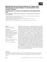
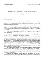
Figure 1. Global geometric representations of plant architecture using a. simple parametric model (from [84]) b. complex parametric
model (from [22]) c. a non-parametric model (from [26]) d. a contour description (from [106]).
C. Godin
416
whose functions are defined by a global model. These
global representations can be divided into two categories.
2.1. Geometric representations
At a global scale, geometric representations of crowns
are used to model plant/environment interactions. Two
types of geometric representations can be distinguished.
A simple and economic representation of plant geome-
try can be constructed using parametric representations.
Spheres or ellipses are used for instance to model light
interception by tree crowns [84] (figure 1a). Cylinders,
cone frustums or paraboloids are used to study the
mechanical properties of plants [6] or in forestry applica-
tions to model trunk or crown shapes e.g. [81]. In order to
account for wider spectra of shapes, these simple paramet-

ric representations can be refined by using more complex
geometric models, i.e. containing slightly more parame-
ters. Cescatti [22], for instance, introduced an asymmetric
geometric model of the tree crown to account for the vari-
ability of crown shapes in a forest stand (figure 1b).
In other studies, flexibility in the geometric represen-
tation is achieved by using non-parametric models.
Cluzeau et al. [26] explored the use of a polyhedral rep-
resentation of crown shape (figure 1c). According to
these authors, such a representation “is intermediate in
terms of computation costs and efficiency between clas-
sical geometric shapes and more elaborated computer
graphic representations”. Another example is provided by
the non-parametric reconstruction of shapes from pho-
tographs. Shimizu and Heins [106] for instance use pho-
togrametry techniques and edge detection algorithms to
compute the connected outlines of a vervain plant from
photographs (figure 1d).
2.2. Compartment representations
Compartment-based approaches are intended to model
exchanges of substances within the plant at a global scale.
Plants are decomposed into two or more compartments
representing sinks or sources for substance transfer within
the plant or at the interface between the plant and its
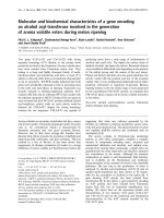
Figure 2. Compartment representations of plant architecture a. in carbon partitioning models. Compartments are represented by dif-
ferent pools of carbon. b. in water transport models, compartments are associated with conductances k (from [123]).
Representing and encoding plant architecture
417
environment. Compartment representations may be con-
sidered as coarse topological descriptions of the plant

architecture. A compartment may, for example, corre-
spond to pools of leaves, roots, fruits or wood with con-
nections between one another. In these pools, the organs
are not differentiated one from another. They are consid-
ered as biomass with certain global properties (photosyn-
thetic efficiency, mass, temperature, transfer rates, etc.).
The first compartment models were introduced to model
the diffusion of assimilates in plants [119, 120]. These
models initially contained a leaf and a root compartment
and described exchanges between these compartments
using differential equations. Since then, compartment
models have undergone substantial development [15, 77,
80, 124] and have given rise to extensions containing addi-
tional compartments to refine the modelling of element
exchanges within the plant. A stem compartment can be
added, for instance, to model the growth process of the
stem and to take into account the consumption of assimi-
lates in the diffusion process [37] (figure 2a). Similarly, to
model water transport, plants are represented as a series of
compartments at the interface between the soil and the
atmosphere. Each compartment has a specific hydraulic
conductivity and the flow of water through the plant results
from the difference in water potential between the surface
of the leaves and the soil/roots [41, 116] (figure 2b).
To summarise, global representations of plant archi-
tecture are representations of either plant geometry or
topology at a coarse scale. They allow the modeller to
design parsimonious models, i.e. models with a small
number of parameters, which in turn favours a biological
interpretation of the model structure. However, for many

applications such as studying microclimate, assimilate
repartition, wood properties, or fruit production in plant
crowns, visualising the branching structure of a plant
architecture, simulating crown development etc., these
models are considered too reductive since they oversim-
plify the plant architecture. In such cases, more complex
representations have to be considered.
3. MODULAR REPRESENTATIONS
This step towards refined representation is based on
the consideration of plants as modular organisms: plants
are made up by the repetition of certain types of compo-
nents [10, 13, 61, 63]. Modular representations rely on the
description of these repeated components. Such represen-
tations are more complex than the global representations
since their specifications are intrinsically longer and usu-
ally contain far more information.
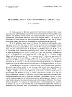
Figure 3. Modular representations of plant architecture a. spatial decomposition. Cells that contain vegetal elements are tagged with
grey. b. organ-based decomposition of the same plant including only geometrical information about leaves. c. organ-based decompo-
sition of the same plant including topological information.
C. Godin
418
Two basic types of plant architecture decompositions
into modules can be carried out: spatial or organ-based
decompositions. In spatial decompositions, the distribu-
tion of plant modules in 3-dimensional space is approxi-
mated by tiling of the 3-dimensional space, using cells
with simple and constant shape and tagging those that
contain plant modules (figure 3a). Organ-based decom-
positions make use of plant modules and can be divided
into two classes: in geometric decompositions, only the

geometric aspects of the modules and their spatial posi-
tions are considered (figure 3b) whereas in topological
representations, the connections between the modules are
taken into account (figure 3c).
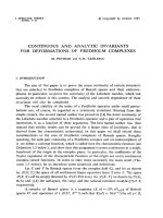
3.1. Spatial representations
Plant modularity can be indirectly exploited by subdi-
viding the space in which the plant is embedded into reg-
ular cells, called voxels (figure 4a). Plant components are
not directly considered in such representations. Instead,
the plant is represented by the voxels containing the plant
components. Biological attributes characterising these
components (leaf density, optical properties, etc.) can be
attached to each voxel. The size of the voxels is deter-
mined according to the application. The plant is repre-
sented in fine by a set of voxels in 3-dimensional space.
Voxel-based representations have been used in the con-
text of light interception modelling, e.g. [111] and plant
growth simulation [59].
3.2. Geometric representations
A second solution consists of decomposing plants into
organs such as leaves, fruits, internodes or different types
of growth units, and considering their shapes and spatial
organisation. The connections between the organs are not
taken into account and not all types of plant organs need
to be considered. One may be interested for example in
the spatial distribution of leaves (e.g. in application deal-
ing with light interception), or roots (e.g. to identify the
areas of water uptake in the soil). These types of modular
representations are frequently used to obtain accurate
descriptions of the plant exchange surface in applications

studying the interaction between plants and their micro-
environment [23, 30, 113] (figure 4b).
3.3. Topological representations
Topological representations are organ-based decom-
positions in which emphasis is placed on the connections
between organs. Such representations are used in an
increasing number of plant structure/function modelling
fields to model either substance transfers within plants,
plant growth or to measure plant architecture. Some
examples of this are given below.
Several models of water fluxes in plants have been
proposed based on an electrical analogy [32, 35, 51]. The
plant is decomposed into components that are associated
with hydraulic conductance. The water flux through a
Figure 4. Representation of plant canopies using a. voxels with varying leaf densities. b. a geometric decomposition of the plant into
leaves (made from digitised grapevine leaves and used to assess irradiance models – from [113]).
Representing and encoding plant architecture
419
component is assumed to be proportional to its conduc-
tance (Ohm’s law). Water transfers within the plant are
thus defined by a “hydraulic network” which relies on the
plant topology: as in the electronic analogy, Kirchhoff’s
current law (see e.g. [25]) is satisfied for each component,
i.e. the flux of water entering a component is equal to the
sum of fluxes leaving.
Plant topology is also used to address carbon partition-
ing problems. In the pipe model theory, for instance, a
plant is considered to be a “bundle of unit pipes”
(figure 5a), each pipe bearing a unit of leaves [83, 108,
124]. Complex branching structures can be represented

by connecting together unit pipes modelling plant com-
ponents. The resulting structure, illustrated in figure 5b,
defines a sapwood network for which Kirchhoff’s current
law is satisfied with the following significance: the num-
ber of unit pipes in a component is equal to the total num-
ber of unit pipes that compose the components connected
above it [88].
Topological representations are also used in a more
abstract manner to simulate the propagation of substances
through plant components. A first problem here consists
Figure 5. Modular description used with the pipe model theory a. Classical representation of a plant in the pipe model theory (from
[107]) b. representation of a branching system with unit pipes: each segment of a tree is represented by a bundle of pipes. A
Kirchhoff’s current law expresses flux conservation c. Tree graph associated with the model from b. Each bundle of pipe is represented
by a vertex and connection between bundles is represented by an edge.
C. Godin
420
of simulating the competition between branches for lim-
iting resources through the plant component network [19,
35]. A second problem lies in the study of signal propa-
gation through plant topology. Such modelling may be
used to explain time of flowering in branching inflores-
cences for example [68].
As computers have become increasingly powerful,
plant growth simulation programs have made extensive
use of the topological representation of plant architecture
to obtain realistic 3-dimensional rendering of computed
plant architectures, e.g. [34, 39, 45, 46, 48, 97, 127]. This
use of 3-dimensional representations was initiated by
Honda [65] who demonstrated that complex crown
shapes could be obtained using a limited number of geo-

metric parameters and that plant architecture is very sen-
sitive to changes in these parameters.
The above list of applications using a topological
representation of plant architecture is naturally not
Figure 6. a. A tree – considered as a set of branches – and b. the tree graph representation of its branch topology c. an oak tree branch-
ing system described in terms of growth-units and d. its corresponding augmented tree graph (from [52]).
Representing and encoding plant architecture
421
exhaustive. However, it is intended to reflect the wide
variety of fields in which plant topology has been adopt-
ed to refine plant representations. All these plant repre-
sentations have a common underlying structure, namely
that of a tree graph.
3.3.1. Tree graphs
Let us consider the set of components resulting from
decomposition of a plant into modules. The network
made by these connected components can be represented
by a binary relation defined over the set of plant compo-
nents, i.e. a graph. Because of the special nature of plant
growth, graphs representing plant topology are of a par-
ticular type [52], known as tree graphs (for an introduc-
tion to graph theory see e.g. [57, 89]). Figures 6a, b
illustrates a tree graph in which each branch is represent-
ed by a vertex and connections between branches are
represented by edges between vertices. Two types of con-
nections can be distinguished to mark the hierarchical
organisation of components in plants. A < (precedes)
denotes the connection between two components that have
been created by the same apical meristem. A + (bears)
denotes the connection between two components that

have been created by different apical meristems.
Additional information can be associated with plant
organs in topological representations by adding features
to the corresponding vertices in the tree graph. This infor-
mation may correspond to the spatial position of an organ
in space, its geometry, or any other characteristic of the
organ. The resulting representation is called an augment-
ed tree graph (figures 6c, d).
A slightly different way of representing plant modu-
larity by a graph, called axial trees, has been proposed by
Prusinkiewicz and Lindenmayer [96] in the context of
plant growth simulation with L-systems. In axial trees,
plants are described as tree graphs where vertices repre-
sent connecting points between plant components and
edges represent the components themselves. This con-
vention mirrors that presented above (vertices in one rep-
resentation are edges in the second and vice versa), and is
equivalent to augmented tree graphs (figures 7a, b).
3.3.2. Computational representation of tree graphs
In all the preceding examples, plant topology can be
modelled by a tree graph whose vertices have different
types of attributes: conductance, water flux, number of
unit pipes, geometry, etc. For example, in the case of unit
pipes, the pipe representation of a tree (figure 5b) can be
alternatively represented as a tree graph (figure 5c),
which emphasises the topology of the tree and defines a
representation independent of the modelling context
(here, independent of the pipes). However, whereas tree
graphs are very general means of representing plant
Figure 7. Equivalence between an axial tree (from [96]) a. and an augmented tree graph b.

C. Godin
422
modularity, there is no universal method to computation-
ally represent them. By contrast, various methods with
specific computational properties may be considered
[2, 57, 118]. A brief description of the major
implementations of tree graphs is given below.
The most commonly-used manner to implement a tree
graph is to use a chained list of records (figure 8). Each
vertex representing a plant component is associated with
a record containing a pointer to the record representing its
parent vertex. Since each vertex in a tree graph has only
one parent at most, a single pointer is needed for each
record. In addition, each record may store further infor-
mation associated with the corresponding vertex (such as
position, geometry, light environment, etc.). This solution
is flexible: new components can easily be added or
removed and the use of memory to describe the topology
is reasonably efficient since the storage of a graph con-
taining N vertices takes a space proportional to N, though
this is not optimal. Also, the search for the parent vertex
of a vertex is very efficient and can be made in constant
time. Variations can be made in such implementations to
reduce either access time or storage space, see e.g. [2,
57];
Tree graphs can also be represented as matrices. Here,
the vertices and the edges of a tree graph are indexed. A
matrix M is considered whose rows and columns are
respectively associated with the vertex and edge indexes.
This matrix is called the incidence matrix of the tree

graph (figure 9). If an edge e is incident to a vertex v and
directed away from vertex v, then cell (v, e) contains 1. If
an edge e is incident at a vertex v and directed toward v,
then cell (v, e) contains –1. Otherwise cell (v, e) contains
0. A matrix representation of graphs can be used to write
equations to describe the flows on these graphs in a syn-
thetic algebraic manner. For instance, Kirchhoff’s current
law can be summarised using the above incidence matrix
by the following equation:
MI = 0
Figure 8. Representation of plant topology by chained lists of
records.
Figure 9. Representation of plant topology by a matrix. a. a tree graph with fluxes going through its nodes (flux i
n
passes through node
n). b. Corresponding incidence matrix: lines correspond to vertices and columns correspond to edges (see text for detailed explanations).
Representing and encoding plant architecture
423
where I is the column vector composed of the value of the
flux entering each vertex in the graph. However, matrix
representations of tree graphs have one major drawback.
Because each vertex in a tree graph is only connected to
a few other vertices, the resulting matrix is sparse, i.e. a
matrix with many null cells (figure 9b). When describing
a plant with a large number of components, this causes
storage problems (the storage of a graph with N vertices
and M edges takes a space proportional to N × M. Since
in a tree, M = N – 1, the space is of the order of magni-
tude of N
2

). However, techniques have been developed in
applied mathematics for efficient computation using
sparse matrices, e.g. [90]. Fourcaud for instance [49, 50],
used a matrix representation and a specific sparse matrix
decomposition scheme to apply efficiently a finite ele-
ment method for modelling the mechanical constraints
within the branches of a growing tree.
Tree graphs can also be represented by strings of char-
acters. This is a common scheme in computer science (a
computer program for instance can be thought of as a
string of characters representing a (tree graph) hierarchy
of expressions). This has proved particularly useful in
plant models based on L-systems (see [92] for a review).
In this case, vertices are represented by letters. To repre-
sent an axis, letters associated with vertices representing
successive components in the axis are concatenated one
after the other. A branch is thus represented by a string of
characters. Axillary branches can be added by inserting
their string representation into the previous string using a
bracket notation (figure 10). A whole branching system is
thus defined by nested strings of characters. String repre-
sentations are concise and provide optimal topology rep-
resentation in terms of storage efficiency (one vertex =
one letter and no pointers are used). However, seeking for
the parent of a component may take a time proportional
to n, n being the length of the string up to the letter asso-
ciated with this component. Thus, computation that
makes use of the topological connections of a component,
for all plant components (e.g. propagating substances
through plant topology), may take a time proportional to

N
2
, N being the number of plant components.
All these implementations of tree graphs can actually
represent a plant architecture within a computer system.
As discussed above, they have different computational
properties, but they can all be used in plant growth simu-
lation programs: a growing architecture will be represent-
ed either by a chained list with an number of records
increasing with time, by a matrix with an increasing num-
ber of rows and columns, or by a string with an increas-
ing length.
3.4. Encoding plant architecture
It is sometimes necessary to represent plant architec-
ture topology in a legible manner. This can be used for
example to describe the topology of a plant observed in
the field or to transfer plant architecture data between two
computer programs. Such encoding schemes rely on the
representation of tree graphs as strings of characters.
Several such encoding strategies have been described
in the literature. Certain strategies have been developed
for specific plant species, e.g. cotton [126] and soybean
[71] (figure 11a). Others are more generic and do not
depend on plant species [62, 101], (figures 11b, c).
However, these approaches focus on a particular plant
modularity, most frequently at the internode or growth
unit levels. These schemes enable the user to describe the
topology of plant individuals. In a slightly different per-
spective, Robinson [102] proposed an encoding scheme
to formalise the description of architectural models [61],

(figure 12).
3.5. Discussion
To conclude this section, let us summarise the advan-
tages and drawbacks of using modular representations in
plant modelling.
Figure 10. String representing a tree graph. Such strings are
used to encode plant architectures.
C. Godin
424
A basic advantage of using modular representations is
directly inherited from the classical analytical method of
tackling complex phenomena: the phenomenon (here the
plant) is decomposed into small components that can be
treated more simply. The phenomenon is then assumed to
be adequately described as the union of these basic com-
ponent models. The hope here is that this will lead to
greater understanding and more accurate modelling of
biological phenomena than use of global representations.
However, this approach has some drawbacks. First, the
use of a modular rather than global representation greatly
increases the size of the plant description. Special tech-
niques must therefore be designed to control the overall
amount of data and computation, e.g. [38]. Second, since
the level at which the plant is described is finer, modellers
frequently attempt to tackle new phenomena that appear
at this more detailed scale. For example, modelling tree
crown geometry at the level of branches requires that the
model integrates some description of the branch distribu-
tion along the trunk. This information need not be taken
into account when using a global model of tree crown

geometry (see Sect. 2). Similarly, models that use an elec-
trical analogy for substance propagation within the tree
structure contain a number of parameters proportional to
the number of plant components. Again, a coarse model
describing substance transfer at the tree scale would be far
Figure 11. Different encoding schemes used to record plant topology in the field. Encoding strategies have been designed for specif-
ic plants a. (soybean plant from [71]) or for general plants b. (from [101] ) and c. (from [62]).
Representing and encoding plant architecture
425
more parsimonious. Therefore, more detailed descriptions
frequently lead to an increase in the size of the model, i.e.
the use of a larger number of parameters. Finally, an addi-
tional shortcoming of modular representations results
from their dependence on the a priori choice of a level of
description. A particular type of module is chosen to rep-
resent a plant and this is frequently determined by the
application aims and constraints. Classical modules are
branching systems, axes, different types of growth-units
and internodes. The plant is then decomposed into com-
ponents corresponding to the repetition of this module in
the plant architecture. The assumption (made explicitly or
not) is that the chosen level of description corresponds to
the optimal level at which the studied phenomenon can be
decomposed into pieces and analysed. This suffers from a
lack of flexibility: first, facts from different levels of
description may be related to the observation of a phe-
nomenon at a given scale. Second, in order to account for
this possibility, modular representations must be modified
to support information from other scales. Systematic
approaches to the integration of phenomena occurring at

different levels of detail in plant architectures have result-
ed in multiscale representations.
4. MULTISCALE REPRESENTATIONS
The first informal multiscale descriptions were used in
architectural analysis where accuracy in architectural
model description is achieved using details from many
different scales. Figure 13 illustrates such multiscale
descriptions [85]. This picture contains details at forest,
tree, branching system, axis and inter-branch segment
scales. The need to formalise such multiscale descriptions
of plant architectures was recently advocated by several
authors [56, 88, 100].
In parallel to the work conducted in architectural
analysis, preliminary attempts were made to quantify
multiscale aspects of plant architecture in the 1980’s,
inspired by a new emerging field of mathematics: fractals
[78, 79]. Mathematicians, e.g. [78, 79], are often reluctant
to give formal definitions of fractals. However, a fractal
object has in general two important properties: it is char-
acterised by irregularities at every scale and has a homo-
geneous mass distribution, e.g. [122]. If the distribution is
heterogeneous, one speaks of multifractal objects [4, 58,
78]. Intuitively the fractal (or multifractal) character of an
Figure 12. Encoding scheme for architectural models (from [102]). O stands for orthotropic, P for Plagiotropic, t for terminal, d for
dichotomous, [O] means determinate unit, (O) indeterminate, etc.
C. Godin
426
object is related to the fact that new details appear when
zooming in on the object. If new details appear at every
scale, the “length” (or surface or volume) of ideal fractal

objects must be infinite (e.g. [82]). A case of particular
importance occurs if fine grain details are similar to
coarse grain details, then the object is said to be self-sim-
ilar (figure 14a).
In the strict sense, branching systems in plants are not
fractal objects. They do have complex structures with
more or less obvious self-similarity [33, 96], but they do
not have infinite length: actually, real plants have a frac-
tal-like aspect only within a limited range of scales
(figure 14b). This property can be brought to light in every
tree-like structure by considering that such structures can
be approximated at scale i by their branches up to order i
and that zooming in on these structures reveals new
details corresponding to order i+1 branches. In this sense,
every branching structure exhibits fractal behaviour, at
least within a certain range of scales (figures 14a, b).
As illustrated by this remark, modelling plants in the
context of fractals has effects on two major aspects of the
modelling strategy. The first concerns the simulation of
Figure 13. Architectural description of a forest showing various levels of detail (from [85]).
Representing and encoding plant architecture
427
plant growth: similarly to fractal object generation, plant
growth can be simulated using a recursive process [86,
94, 114]. The second, central to our subject, concerns the
nature of the plant structure itself: similarly to fractal
objects, the plant structure contains details at different
scales of description.
For plants as for fractals, we may define a notion of
scale from the process of tiling an object using some cho-

sen measurement unit [58, 78, 122]. A scale (of descrip-
tion) is defined by the choice of a unit used to tile up the
object (here a plant). The finer the unit, the finer the
description (i.e. the higher the scale of description). In
this sense, we can speak of the description of a plant at the
annual shoot scale (for instance), meaning that the plant
has been decomposed and described (tiled) in terms of its
annual shoots.
The architectural or fractal approach (or sometimes
both) have been at the origin of attempts to represent mul-
tiscale phenomena within tree crowns since the 1980’s.
Both result in different types of multiscale representa-
tions of plant architecture that are reviewed hereafter. As
already seen for modular representations, these approach-
es can be divided into three categories depending on the
type of multiscale decomposition, i.e. either spatial, geo-
metric or topological.
4.1. Multiscale spatial representations
The first type of representation consists of decompos-
ing the Euclidean space into voxels of varying sizes. The
size of any voxel is adapted to local shape irregularity: the
more irregular the shape, the finer the voxels. Such hier-
archical data structures have been used for many years in
engineering to deal with partial differential equations
using finite or discrete element methods on domains with
complex shapes (e.g. [98]). A similar tiling is also used to
Figure 14. a. Self-similar formal tree resulting from a fractal process. The theoretical output is a fractal object, i.e. it has details at
every scale and has an infinite length (from [82]) b. Virtual and realistic tree obtained from a fractal process (e.g. [125], Photo by
Viennot).
C. Godin

428
compute the Hausdorff dimension of a fractal object (e.g.
[42]). Recently, Sillion et al. adapted a hierarchical
approach of radiosity methods to model the energy
exchanges between vegetation elements [28, 109]. To
increase the efficiency of radiosity methods, plant archi-
tecture is decomposed into voxels of different sizes and
radiosity properties corresponding to the actual vegeta-
tion elements they contain. An octree technique is used to
locally adapt the size of the voxels to the level of detail of
the plant components (figure 15).
4.2. Multiscale geometric representations
A second type of representation consists of decompos-
ing the global shape into smaller shapes, and so on until
the desired level of accuracy is obtained. Zeide [130, 131]
used such multiscale geometric decompositions in
forestry applications to characterise the complex shape of
forest-tree crowns, assumed to have a fractal nature, by
comparing the surface of the geometric representations of
trees at different scales, see “the two surface method”
Figure 15. Multiscale voxel-space: the plant architecture is approximated by voxels whose sizes are locally adapted to the irregulari-
ty of the plant geometry (From [109]).
Representing and encoding plant architecture
429
[129]. Multiscale geometric representations have recently
been used in computer graphics to model the complex
geometry of biological organs in a hierarchical manner
[7]. These methods are currently being investigated to
introduce multiscale geometric representations of tree
crowns to model radiative transfers in canopies.

4.3. Multiscale topological representations
The fractal aspect of plant architectures has lead sev-
eral researchers to design plant growth simulation sys-
tems using fractal concepts such as self-similarity, scale,
recursion, dimension, etc. [24, 86, 94, 114, 125], (e.g.
figure 14b). In these approaches, the plant representation
is not fundamentally different from that used in modular
approaches. The fractal aspect of these approaches lies in
the recursive process that generates a self-similar struc-
ture in a few steps [9, 92]. Like for modular approaches,
the plant topology is represented by a tree graph, using a
single “unit” of description (for instance internodes).
Increasing levels of detail are expressed by additional
branching structures, e.g. by increasing branching orders
(figure 16).
In the 1990’s, other types of multiscale plant represen-
tations were introduced, making explicit the existence of
entities at different levels of detail. Relying on architec-
tural analysis concepts, AMAP simulation software uses
a layered data structure where different types of plant
component are represented at different scales: internode,
growth unit, axis and reiteration [17, 66] (figure 17). This
data structure is used in plant growth simulation to adapt
meristem production to the nature (age, order and physi-
ological state) of their embedding growth unit and axis. A
similar plant representation is used in INCA [74] where
the paradigm of expert systems is used to model the plant
growth process. This growth is governed by a set of rules
(written in Prolog) expressing the conditions of meristem
growth and differentiation as a function of the physiolog-

ical state of the plant components at different scales. In
Figure 16. Developmental sequence of a branching system
modelled using a tD0L-system (from [96]). New details corre-
spond to new branching orders.
Figure 17. Organisation of records representing plant architecture in AMAPpara software (from [18]).
C. Godin
430
turn, the multiscale data structure representing plant
architecture is updated with new physiological values and
with new components at different scales.
Multiscale plant models can also be found in object-
oriented approaches. Here, the intention is to describe the
structural-functional properties and the relationships
between the components as closely to reality as possible.
The emphasis is therefore on the design of objects that
represent plant components. In object–oriented approach-
es, objects are more than simple data structures in the
sense that objects also define the manner in which the
data they contain may be accessed and used (e.g. [64]).
Salminen et al. [105] used an object-oriented approach to
specify the nature of plant components at different scales
and determine their structural and functional connections
(figure 18a). With such a specification, the simulation
program builds up a plant representation which contains
components at different levels of detail, i.e. a multiscale
data structure (figure 18b). Here, it is expected that emer-
gent properties (such as plant morphology, trunk volume,
crown aspect, etc.) will derive from a local but detailed
modelling of the interaction between plant components.
These approaches were designed to account for inter-

actions occurring between components at different scales
during plant growth simulations and did not place much
emphasis on the multiscale representation of the plant
itself. Godin and Caraglio [52] formalised the notion of
growing multiscale structures and studied their mathemat-
ical properties. The resulting plant architecture represen-
tation model is called a multiscale tree graph (MTG) and
is the multiscale counterpart of the tree graph model
described in the previous section. Following the definition
of the notion of scale used in fractal geometry (see above),
a scale in a MTG is associated with a unit of decomposi-
tion. In figure 19 the plant has been decomposed at three
different scales corresponding to three units of decompo-
sition, axis, growth units and internode. At each scale, the
plant structure is represented by a tree graph. All these tree
graphs are integrated within a MTG by making explicit
the decomposition relationships between the components.
Figure 18. Object oriented approach. a. Formal specification of the functions and structural relationships between plant organs (from
[105]) b. Plant architecture representation produced by a program using such an object-oriented specification. The different types of
grey levels represent the different types of objects as defined in a.
Representing and encoding plant architecture
431
Figure 19. Multiscale tree graphs. The plant can be represented by a tree graph at different scales, e.g. axis scale a. growth unit scale
b. and internode scale c. A multiscale-tree graph result from the superposition of all these representations d. (from [52]).
C. Godin
432
A growing plant is represented by a time-varying MTG
where each tree graph at any scale is a growing tree graph.
Using this formalism, Godin and Caraglio showed that
decomposition relationships between components during

plant growth may vary over time (figure 20). This proper-
ty can be used to model the growth of complex structures.
MTGs are used in AMAPmod software dedicated to plant
architecture measurement and analysis [53, 55, 56], as a
central data structure used to organise all the information
collected on plants.
4.4. Multiscale structure encoding
Multiscale representation of plant architecture is a
rather recent issue in plant architecture modelling. Little
work has been carried out on encoding such multiscale
representations. For plants whose multiscale architecture
is generated using fractal-based mechanisms or L-sys-
tems, the first possibility consists of reusing the string
notation for encoding tree graphs (see Sect. 3). The com-
plete string represents the plant containing a maximum of
details. From this detailed description, plant description
at a coarser scale can be obtained by removing substrings
included between square brackets corresponding to high
levels of detail from the initial string.
A special encoding scheme has been designed for
MTGs to describe the multiscale topology of plants
observed in the field [53] (figure 21). Recently, this
scheme has been extended to integrate the description of
component geometry in a consistent way within the mul-
tiscale representation using 3D digitising [27, 54, 112]. A
plant described in this manner can be reconstructed
(figure 22) and analysed using AMAPmod software.
5. DISCUSSION
In this paper, a wide variety of models for representing
plant architectures have been outlined, ranging from

global to multiscale representations. These models
have been shown to correspond to a few formal
Figure 20. Variation of the decomposition relationship with time in the topological description of a branching system (illustration on
the differentiation of a reiterated complex from the trunk of a plant). A trunk is made of several components, here modules for instance.
During plant growth, any macroscopic component (such as the trunk (t
1
)) may lose some of its components (in black (t
2
)) to the ben-
efit of new macroscopic components (t
3
) (e.g. a reiterated complex) (from [52]).
Representing and encoding plant architecture
433
representations. Tree graph representations are at the core
of modular representations (when topology is taken into
account) whereas multiscale tree graph representations
play a similar role for multiscale representations.
The three types of plant architecture representation
described in this paper, namely the global, modular and
multiscale representations, actually correspond to an
increasing degree of robustness.
Non-robust models are those that work solely for the
goal for which they were initially designed. A change of
goal requires at least a modification in the model or more
drastically a change of model. This is the case for
instance in global models which reduce to a minimum the
plant representation, taking account of the modelling
objective and nothing more. Because of their restricted
range of use, non-robust models are often concise. By

contrast, robust models have the ability to adapt to objec-
tives for which they were not initially designed. In this
sense, modular representations of plant architecture are
more robust than global representations since the decom-
position of the architecture into basic components makes
it possible to support more applications. They are, how-
ever, less concise.
If we assume, for example, that the geometrical
parameters for every component in the modular represen-
tation of a plant’s architecture are known, this representa-
tion may be used without modification in various
applications: estimating light interception in crowns [31,
113, 117], modelling water/assimilate fluxes through the
plant architecture [32, 51], realistic 3D rendering of
plants [34, 95], modelling the mechanical strengths in
branches [50], computing the distribution of component
geometric and topological characteristics in crowns [27]
or in root systems [29, 70, 87], making spatial statistics in
the tree crown [5], studying the motion of insects on
stems [62], estimating the distribution of water under a
vegetal canopy during rain, modelling the node structure
in log sections [67], and more. The robustness of modu-
lar representations is a key factor supporting their
increasingly frequent use in modelling applications.
Figure 21. Encoding multiscale plant architecture representations. a. the plant is decomposed into components at different scales. b.
A MTG formally represents this decomposition c. The MTG is encoded using a string notation [53].
C. Godin
434
Multiscale representations are even more robust than
modular representations since they contain more structur-

al information. They potentially allow the user to address
different scales of space or time within a modelling appli-
cation. However, they are also more complex, which lim-
its their current use in plant modelling. Nonetheless,
current research in plant modelling highlights the need to
integrate information at different scales in plant architec-
ture representations [8, 27, 56, 88, 100]. Such a growing
consensus should favour the use of multiscale representa-
tion of plants in future structure/function models. This
will only be the case if adequate tools and models are
built to handle these complex plant representations.
As underlined by this review of the literature, modular
representations are currently the most widely used repre-
sentation in plant structural-functional modelling. They
currently correspond to the best compromise between
complexity and robustness. However, the interest in
developing global or multiscale representations is
increasing. On the one hand, scaling up models from
plant individuals to forest stands requires global and effi-
cient representations of plant architecture. On the other
hand, a detailed understanding of plant growth, at differ-
ent time scales, relies on the modelling of plant architec-
ture at different spatial scales.
The choice of a plant architecture representation is
often associated with the problem of collecting plant
architecture data in the field. This can be used either to
analyse different types of distributions within plant archi-
tecture, to define reference data for building plant struc-
ture/function models or initial data for simulations of
plant growth, or to assess model output compared with

actual data. The increasing interest of the research com-
munity in plant structure/function models makes the
collection of plant architecture data an increasingly
important issue. However, collecting architecture data
requires the definition of complex experimental and
observation protocols. This is a time-consuming task (e.g.
Figure 22. Side and top view of a digitised tree in a multiscale context. The representation contains both geometric and multiscale topo-
logical information. Fruit attributes (like red colouring or “blush”) can be analysed according to their architectural context (from [27]).
Representing and encoding plant architecture
435
[54]) and the apparent heterogeneity of plant architecture
representations, discussed above, makes it difficult to col-
lect architecture information in the field in a reusable
way.
The research community currently lacks such reusable
databases and associated tools. However, we have shown
in this paper that there are actually only a few different
formalisms to represent plant architecture and that tools
to deal with such representations are emerging, e.g. [1,
43, 54, 55, 62, 72, 75, 91, 93]. This suggests that a task of
primary importance for the plant modelling community is
to define i) translation schemes to exchange plant archi-
tecture data and ii) common data formats and tools to cre-
ate standard plant architecture database systems that
could be shared by research teams, with different model-
ling goals, throughout the world.
Acknowledgements: I would like to thank E. Costes,
H. Sinoquet, Y. Guédon and F. Houllier and for their
fruitful comments on the first version of this paper.
REFERENCES

[1] Adam B., Sinoquet H., Godin C., 3A version 1.0 : Un
logiciel pour l’Acquisition de l’Architecture des Arbres, inté-
grant la saisie simultanée de la topologie au format AMAPmod
et de la géométrie par digitalisation 3D, Guide de l’utilisateur,
Clermont-Ferrand, France, INRA-PIAF, 1999.
[2] Ahuja R.K., Magnanti T.L., Orlin J.B., Network flows.
Theory, algorithms, and applications, Prentice Hall, Upper
Saddle River, New Jersey, USA, 1993.
[3] André J.P., A study of vascular organization of Bamboos
(Poaceae-Bambuseae) using a microcasting method, IAWA
Journal 19, 3 (1998) 265-278.
[4] Arneodo A., Argoul F., Bacry E., Elezgaray J., Muzy
J.F., Ondelettes, multifractales et turbulences – de l’ADN aux
croissances cristallines, Diderot Editeur, Paris, France, 1995.
[5] Audergon J.M., Monestiez P., Habib R., Spatial depen-
dences and sampling in a fruit tree: a new concept for spatial
prediction in fruit studies, J. Horticult. Sci. 68, 1 (1993) 99-112.
[6] Baker C.J., The development of a theoretical model for
the windthrow of plants, J. Theor. Biol. 175, 3 (1995) 355-372.
[7] Banegas F., Michelucci D., Roelens M., Jaeger M.,
Canovas F., Hierarchical automated clustering of cloud point set
by ellipsoidal skeleton, Application to organ geometric model-
ing from CT-scan images, in: SPIE’s International Symposium
on Medical Imaging 1999, San Diego, USA, 1999, in press.
[8] Barczi J.F., de Reffye P., Caraglio Y., Essai sur l’identi-
fication et la mise en oeuvre des paramètres nécessaires à la
simulation d’une architecture végétale : le logiciel AMAPsim,
in: Bouchon J., de Reffye P., Barthélémy D. (Eds.),
Modélisation et Simulation de l’Architecture des Végétaux,
INRA Éditions, Paris, France, 1997, pp. 205-254.

[9] Barnsley M.F., Fractals everywhere, Academic press,
Boston, 1988.
[10] Barthélémy D., Edelin C., Halle F., Architectural con-
cepts for tropical trees, in: Holm-Nielsen L.B., Nielsen I.C.,
Balslev E. (Eds.), Symposium on Tropical Forests, Academic
Press, London, Aarhus, Danemark, 1989, pp. 89-100.
[11] Barthélémy D., Edelin C., Halle F., Canopy architec-
ture, in: Raghavendra A.S. (Ed.) Physiology of trees, John
Wiley and Sons Inc., 1991, pp. 1-20.
[12] Bell A.D., The simulation of branching patterns in mod-
ular organisms, Phil. Trans. R. Soc. London 313 (1986) 143-
159.
[13] Bell A.D., Plant form, An illustrated guide to flowering
plant morphology, Oxford University Press, Oxford, 1991.
[14] Bell A.D., Roberts D., Smith A., Branching patterns: the
simulation of plant architecture, J. Theor. Biol. 81 (1979) 351-
375.
[15] Bertin N., Environnement climatique, compétition pour
les assimilats et modélisation de la nouaison de la tomate en cul-
ture sous serre, Ph.D. Thesis, INRA, Paris Grignon, 1993.
[16] Birnbaum P., Modalités d’occupation de l’espace par les
arbres en forêt guyanaise, Ph.D. Thesis, Université Paris VI,
Paris, France, 1997.
[17] Blaise F., Simulation du parallélisme dans la croissance
des plantes et applications, Ph.D. Thesis, Université Louis
Pasteur (ULP), Strasbourg, France, 1991.
[18] Blaise F., Barczi J.F., Jaeger M., Dinouard P., de Reffye
P., Simulation of the growth of plants. Modeling of metamor-
phosis and spatial interactions in the architecture and develop-
ment of plants, in: Kunii T.L., Luciani A. (Eds.), Cyberworlds,

John Wiley & Sons, Ltd, Tokyo, Japon, 1998, pp. 81-109.
[19] Borchert R., Honda H., Control of development in the
bifurcating branch system of Tabeduia rosea: a computer simu-
lation, Botanical Gazette 145, 2 (1985) 184-195.
[20] Bouchon J., de Reffye P., Barthélémy D. (Eds.),
Modélisation et simulation de l’architecture des végétaux,
INRA Éditions, Paris, France, 1997.
[21] Caraglio Y., Edelin C., Architecture et dynamique de la
croissance du platane, Platanus hybrida Brot. (Platanaceae)
{syn. Platanus acerifolia (Aiton) Willd.}, Bulletin de la Société
Botanique de France, Lettres botaniques 137, 4-5 (1990) 279-
291.
[22] Cescatti A., Modelling the radiative transfer in discon-
tinuous canopies of asymmetric crowns. I. Model structure and
algorithms, Ecol. Modell. 101 (1997) 263-274.
[23] Chelle M., Développement d’un modèle de radiosité
mixte pour simuler la distribution du rayonnement dans les cou-
verts végétaux, Ph.D. Thesis, Université de Rennes I, Rennes,
France, 1997.
[24] Chen S.G., Ceulemans R., Impens I., A fractal-based
Populus canopy structure model for the calculation of light
interception, For. Ecol. Manag. 69, 1-3 (1994) 97-110.
[25] Chen W.K., Applied graph theory, North Holland Publ.
Co., Amsterdam, The Netherlands, 1976.
[26] Cluzeau C., Dupouey J.L., Courbaud B., Polyhedral
representation of crown shape, A Geometric tool for growth
modelling, Ann. Sci. For. 52 (1995) 297-306.
[27] Costes E., Sinoquet H., Godin C., Kelner J.J., 3D digi-
tizing based on tree topology: application to study the variabili-
ty of apple quality within the canopy, Acta Horticulturae (1999)

in press.
C. Godin
436
[28] Damez C., Application de la méthode de radiosité aux
simulations botaniques, Mémoire de DEA Imagerie, vision et
Robotique, Paris, INAPG, 1998.
[29] Danjon F., Sinoquet H., Godin C., Colin F., Drexhage
M., Characterisation of structural tree root architecture using 3D
digitising and AMAPmod software, Plant Soil 211, 2 (1999)
241-258.
[30] Dauzat J., Simulated plants and radiative transfer simu-
lations, in: Varlet-Grancher C., Bonhomme R., Sinoquet H.
(Eds.), Colloque Structure du Couvert Végétal et Climat
Lumineux: méthodes de caractérisation et applications, INRA
Editions, Saumane, France, 1993, pp. 271-278.
[31] Dauzat J., Eroy M.N., Simulating light regime and inter-
crop yields in coconut based farming systems, Eur. J. Agron. 7
(1997) 63-74.
[32] Dauzat J., Rapidel B., Berger A., Simulation of leaf
transpiration and sap flow in virtual plants: description of the
model and application to a coffee plantation in Costa Rica,
Agricult. For. Meteor. (1999) in press.
[33] de Reffye P., Dinouard P., Barthélémy D., Architecture
et modélisation de l’Orme du Japon Zelkova serrata (Thunb.)
Makino (Ulmaceae): la notion d’axe de référence, in: De la
forêt cultivée à l’industrie de demain, 3
e
Colloque Sciences et
Industries du Bois, Arbora, Bordeaux, France, 1990, pp. 351-
352.

[34] de Reffye P., Edelin C., Françon J., Jaeger M., Puech C.,
Plant models faithful to botanical structure and development, in:
SIGGRAPH’88, Atlanta, USA, 1988, pp. 151-158.
[35] de Reffye P., Fourcaud T., Blaise F., Barthélémy D.,
Houllier F., A functional model of tree growth and tree archi-
tecture, Silva Fenn. 31, 3 (1997) 297-311.
[36] de Reffye P., Houllier F., Blaise F., Fourcaud T., Essai
sur les relations entre l’architecture d’un arbre et la grosseur de
ses axes végétatifs, in: Bouchon J., de Reffye P., Barthélémy D.
(Eds.), Modélisation et Simulation de l’Architecture des
Végétaux, INRA Éditions, Paris, France, 1997, pp. 255-423.
[37] Deleuze C., Houllier F., A transport model for tree ring
width, Silva Fenn. 31, 3 (1997) 239-250.
[38] Deussen O., Hanrahan P., Lintermann B., Mech R.,
Pharr M., Prunsinkiewicz P., Realistic modeling and rendering
of plant ecosystems, in: SIGRAPPH’98, ACM, Orlando,
Florida, USA, 1998.
[39] Diggle A.J., ROOTMAP-A model in three-dimensional
coordinates of the growth and structure of fibrous root systems,
Plant Soil 105 (1988) 169-178.
[40] Edelin C., The monopodial architecture: the case of
some trees species from tropical Asia, Research Pamph. 105
(1990).
[41] Ewers F.W., Cruiziat P., Measuring water transport and
storage, in: Lassoic J.P., Hinckley T.M. (Eds.), Techniques and
approaches in forest tree physiology, CRC Press, Boca Raton,
USA, 1991, pp. 91-115.
[42] Falconer K., Fractal geometry: mathematical foundation
and applications, John Wiley & Sons, Chichester, 1990.
[43] Ferraro P., Godin C., A distance measure between plant

architectures, Ann. For. Sci. 57 (2000) 445-461.
[44] Fisher J.B., How predictive are computer simulations of
tree architecture?, Int. J. Plant Sci. 153, 3 (1992) 137-146.
[45] Fisher J.B., Weeks C.L., Tree architecture of Neea
Nyctaginaceae: geometry and simulation of branches and the
presence of two different models, Bull. Mus. Hist. Nat. 7 (1985)
385-401.
[46] Fitter A.H., The topology and geometry of plant root
systems: influence of watering rate on root system topology in
Trifolium pratense, Ann. Botany 58 (1986) 91-101.
[47] Fitter A.H., An architectural approach to the compara-
tive ecology of plant root systems, New Phytologist 106
(Suppl.) (1987) 61-77.
[48] Ford E.D., Avery A., Ford R., Simulation of branch
growth in the Pinaceae: interactions of morphology, phenology,
foliage productivity, and the requirement for structural support,
on the export of carbon, J. Theor. Biol. 146 (1990) 15-36.
[49] Fourcaud T., Analyse du comportement mécanique
d’une plantes en croissance par la méthode des éléments finis,
Ph.D. Thesis, Université de Bordeaux I, Bordeaux, France,
1995.
[50] Fourcaud T., Lac P., Mechanical analysis of the form
and internal stresses of a growing tree by the finite element
method, in: Engin A.E. (Ed.) PD-Vol. 77, Engineering Systems
Design Analysis Proceedings, ASME, 1996, pp. 213-220.
[51] Früh T., Simulation of water flow in the branched tree
architecture, Silva Fenn. 31, 3 (1997) 275-285.
[52] Godin C., Caraglio Y., A multiscale model of plant
topological structures, J. Theor. Biol. 191 (1998) 1-46.
[53] Godin C., Costes E., Caraglio Y., Exploring plant topol-

ogy structure with the AMAPmod software: an outline, Silva
Fenn. 31, 3 (1997) 355-366.
[54] Godin C., Costes E., Sinoquet H., A method for describ-
ing plant architecture which integrates topology and geometry,
Ann. Botany 84 (1999) 343-357.
[55] Godin C., Guédon Y., Costes E., Exploration of plant
architecture databases with the AMAPmod software illustrated
on an apple-tree hybrid family, Agronomie 19, 3-4 (1999) 163-
184.
[56] Godin C., Guédon Y., Costes E., Caraglio Y.,
Measuring and analyzing plants with the AMAPmod software,
in: Michalewicz M.T. (Ed.) Plants to ecosystems – Advances in
Computational Life Sciences, 2nd International Symposium on
Computer Challenges in Life Science, CSIRO Australia,
Melbourne, Australia, 1997, pp. 53-84.
[57] Gondran M., Minoux M., Graphs and algorithms,
Wiley-Interscience, New-York, 1984.
[58] Gouyet J.F., Physique et structures fractales, Masson,
Paris, France, 1992.
[59] Greene N., Voxel space automata: modeling with sto-
chastic growth processing in voxel space, Comp. Graph. 23, 3
(1989) 175-184.
[60] Hallé F., Modular growth in seed plants, Phil. Trans. R.
Soc. London 313 (1986) 77-87.
[61] Hallé F., Oldeman R.A.A., Tomlinson P.B., Tropical
trees and forests, An architectural analysis, Springer-Verlag,
New-York, 1978.
[62] Hanan J.S., Room P.M., Practical aspects of plant
research, in: Michalewicz M.T. (Ed.) Plants to ecosystems –
Advances in Computational Life Sciences, 2nd International

Symposium on Computer Challenges in Life Science, CSIRO
publishing, Melbourne, Australia, 1997, pp. 28-43.
Representing and encoding plant architecture
437
[63] Harper J.L., Rosen B.R., White J., The growth and form
of modular organisms, The Royal Society, London, UK, 1986.
[64] Hill D.R.C., Object-oriented analysis and simulation,
Addison-Wesley Publ. Co., Harlow, UK, 1996.
[65] Honda H., Description of the form of trees by the para-
meters of the tree-like body: Effects of the branching angle and
the branch length on the shape of the tree-like body, J. Theor.
Biol. 31 (1971) 331-338.
[66] Jaeger M., Représentation et simulation de la croissance
des végétaux, Ph.D. Thesis, Université Louis Pasteur (ULP),
Strasbourg, France, 1987.
[67] Jaeger M., Leban J.M., Chemouny S., Saint André L.,
3D stem reconstruction from CT scan exams, in: Biological
improvement of wood properties, Third Workshop IUFRO WP
S5.01-04, La Londe-Les-Maures, France, 1999, accepted.
[68] Janssen J.M., Lindenmayer A., Models for the control
of branch positions and flowering sequences of capitula in
Mycelis muralis (L.) Dumont (Compositae), New Phytologist
105 (1987) 191-220.
[69] Johnson R.S., Lakso A.N., Approaches to modeling
light interception in orchards, HortScience 26, 8 (1991) 1002-
1004.
[70] Jourdan C., Rey H., Modelling and simulation of the
architecture and development of the oil-palm (Elaeis guineensis
Jacq.) root system. I. The model, Plant Soil 190 (1997) 217-233.
[71] Keisling T., Counce P., An encoding process for mor-

phological analysis of soybean fruit distribution, Crop Sci. 37
(1997) 1665-1669.
[72] Kurth W., Growth grammar interpreter GROGRA 2.4:
A software for the 3-dimentional interpretation of stochastic,
sensitive growth grammar in the context of plant modelling,
Introduction and Reference Manual, Forschungszentrum
Waldokosysteme der Universitat Gottingen, 1994.
[73] Kurth W., Morphological models of plant growth: pos-
sibilities and ecological relevance, Ecol. Modell. 75-76 (1994)
299-308.
[74] LeDizès S., Cruiziat P., Lacointe A., Sinoquet H.,
LeRoux X., Balandier P., Jacquet P., A Model for simulating
structure-function relationships in walnut tree growth processes,
Silva Fenn. 31 (1997) 313-328.
[75] Lewis P., 3-D plant modelling for remote sensing simu-
lation studies using the Botanical Plantb Modelling System,
Agronomie 19, 3-4 (1999) 185-210.
[76] Luck H.B., Luck J., Modélisation du fonctionnement
d’un méristème par des L-systèmes et des systèmes de graphes
et de cartes à réécriture parallèle, in: Le Guyadère H. (Ed.),
Masson, Paris, France, 1987, pp. 375-395.
[77] Mäkelä A.A., Sievänen R.P., Comparison of two shoot-
root partitioning models with respect to substrate utilization and
functional balance, Ann. Botany 59 (1987) 129-140.
[78] Mandelbrot B.B., The fractal geometry of nature, W.N.
Freeman, New York, USA, 1983.
[79] Mandelbrot B.B., Fractals, in: Meyers R.A. (Ed.)
Encyclopedia of physical science and technology, Academic
Press, Orlando, Florida USA, 1987.
[80] McMurtrie R.E., Forest productivity in relation to car-

bon partitioning and nutrient cycling: a mathematical model, in:
Cannell M.G.R., Jackson J.E. (Eds.), Attributes of trees as crops
plant, ITE, Monks Wood, Abbots Ripton, Hunts, UK, 1985,
pp. 194-207.
[81] Mitchell K.J., Dynamics and simulated yield of
Douglas-fir, For. Sci. 21, 4 (1975) 1-39.
[82] Newman W.I., Turcotte D.L., Gabrielov A.M., Fractal
trees with side branching, Fractals 5, 4 (1997) 603-614.
[83] Nikinmaa E., Analyses of the growth of scots pine;
matching structure with function, Acta For. Fenn. 235 (1992) 3-
68.
[84] Norman J.M., Welles J.M., Radiative transfer in an
array of canopies, Agronomy J. 75 (1983) 481-488.
[85] Oosterhuis L., Oldeman R.A.A., Sharik T.L.,
Architectural approach to analysis of North American temperate
deciduous forests, Canadian J. For. Res. 12, 4 (1982) 835-847.
[86] Oppenheimer P.E., Real time design and animation of
fractal plants and trees, in: Evans D.C., Athay R.J. (Eds.), SIG-
GRAPH’86, ACM, Dallas, Texas USA, 1986, pp. 55-64.
[87] Pagès L., Root system architecture: from its represen-
tion to the study of its elaboration, Agromonie 19, 3/4 (1999)
295-304.
[88] Perttunen J., Sievänen R., Nikinmaa E., Salminen H.,
Saarenmaa H., Väkevä J., LIGNUM: a tree model based on sim-
ple structural units, Ann. Botany 77 (1996) 87-98.
[89] Preparata F., Yeh R., Introduction to discrete structures
for computer science and engineering, Addison-Wesley,
Reading Menlo Park London, 1973.
[90] Press W.H., Teukolsky S.A., Vetterling W.T., Flannery
B.P., Numerical recipes in C. The art of scientific computing,

2nd ed., Cambridge University Press, Cambridge, 1996.
[91] Prusinkiewicz P., (project leader), Virtual Plant
Laboratory. A hypertext document and software distribution,
/>(1996).
[92] Prusinkiewicz P., Modeling of spatial structure and
development of plants: a review, Scientia Horticult. 74 (1998)
113-149.
[93] Prusinkiewicz P., Hammel M., Hanan J., Mech R., L-
system: from the theory to visual models of plants, in:
Michalewicz M.T. (Ed.) Plants to Ecosystems. Advances in
Computational Life Sciences, I, CSIRO publishing, Melbourne,
1997, pp. 1-27.
[94] Prusinkiewicz P., Hanan J., Lindenmayer systems, frac-
tals, and plants, Springer Verlag, New-York, 1989.
[95] Prusinkiewicz P., James M., Mech R., Synthetic topiary,
in: Computer Graphics Proceedings, 1994, pp. 351-358.
[96] Prusinkiewicz P., Lindenmayer A., The algorithmic
beauty of plants, Springer Verlag, New York, 1990.
[97] Prusinkiewicz P., Remphrey W.R., Davidson C.G.,
Hammel M.S., Modeling the architecture of expanding Fraxinus
pennsylvanica shoots using L-systems, Canadian J. Botany 72
(1994) 701-714.
[98] Rao S.S., The finite element method in engineering., 3rd
ed, Butterworth Heinemann, Boston, USA, 1999.
[99] Remphrey W.R., Neal B.R., Steeves T.A., The mor-
phology and growth of Arctostaphylos uva-ursi bearberry: an
architectural model simulating colonizing growth, Canadian J.
Botany 61 (1983) 2451-2458.