Báo cáo toán học: "Enumeration of Pin-Permutations" pdf

Enumeration of Pin-Permutations
∗
Fr´ed´erique Bassino
LIPN UMR 7030, Universit´e Paris 13 and CNRS,
99, avenue J B. Cl´ement, 93430 Villetaneuse, France.
Mathilde B ouvel
LaBRI UMR 5800, Universit´e de Bordeaux and CNRS,
351, cours de la Lib´eration, 33405 Talence cedex, France.
Dominique Rossin
LIX UMR 7161, Ecole Polytechnique and CNRS,
91128 Palaiseau, France.
Submitted: Dec 19, 2008; Accepted: Feb 28, 2011; Published: Mar 11, 2011
Mathematics Subject Classification: 05A15, 05A05
Abstract
In this paper, we study the class of pin-permutations, that is to say of per-
mutations having a pin representation. This class has been recently introduced in
[16], where it is used to find properties (algebraicity of the generating function,
decidability of membership) of classes of permutations, depending on th e simple
permutations this class contains. We give a recursive characterization of the sub-
stitution decomposition trees of pin-permutations, which allows us to compute the
generating function of this class, and consequently to prove, as it is conjectured in
[18], the rationality of this generating function. Moreover, we show that the basis
of the pin-permutation class is infinite.
1 Introduction
In the combinatorial study of permuta t io ns, simple permutati ons have been the core
objects of many recent works [2, 3, 1 5, 16, 17, 18, 20]. These simple permutations are
the “building blocks” on which all permutations are built, through their sub stitution
decomposition. Recently, substitution decomposition of permutations has also been used
to exhibit relations between the basis of permutation classes, and the simple permutations
∗
This work was completed with the support of the ANR (projects GAMMA BLAN07-2 195422 and

MAGNUM ANR-2010-BLAN-0204).
the electronic journal of combinatorics 18 (2011), #P57 1
this class contains [2, 16, 17, 18]. Similar decompositions for other objects have been
widely used in the literature: for relations [25, 26, 32, 34], for graphs [13, 36], or in a
variety o f other fields [19, 22, 35].
In the algorithmic field, the substitution decomposition (or interval decomposition) of
permutations has been defined in [5, 6, 38]. It takes its roots in the modular decomposition
of graphs (see for example [13, 21, 29, 36, 37]), where prime graphs play the same key
role as simple permutations. Some examples of an algorithmic use of the substitution
decomposition of permutations ar e the computation of the set of common intervals of
two (or more) permutations [6, 38], with applications to bio-informatics [5], or restricted
versions of the longest common patt ern problem among permutations [8, 11, 12, 28].
In the study of substitution decomposition, ther e is a major difference between algo-
rithmics and combinatorics: algorithms proceed through the substi tution decomposition
tree of permutations, that is to say recursively decompose every block appearing in the
substitution decompo sition of a permutation. On the contrary, in combinatorics, the sub-
stitution decomposition is mostly interested in the skeleton of the permutation, which
corresponds to the root of its decomposition tree.
In the present work, we take advantage of both points of view, and use the substitution
decomposition tree with a combinatorial pur pose. We deal with permuta tions that ad-
mit pin representations, denoted pin-permuta tion s . These permutations were introduced
recently by Brignall et al. in [16] when studying the links between simple permutations
and classes of pattern-avoiding permutations, from an enumerative point of view. The
authors conjectured in [18] that the class of pin-permutations has a rational generating
function. We prove this conjecture, focusing on the substitution decomposition trees of
pin-permutations.
In Section 2, we start with recalling the definitions of substitution decomposition and
of pin-permuta tions, and describe some of their basic properties. The core of this work
is the proof of Theorem 3.1 which gives a complete char acterization of the decomposition
trees of pin-permutations. This corresponds to Section 3. Section 4 focuses on the enu-

meration of simple pin-permutations, using the notion of pin words defined in [18]. With
this enumerative result and the characterization of Theorem 3.1, standard enumerative
techniques [24] allow us to obtain the gener ating function of the pin-permutation class
in Section 5. This generating function being rational, this settles a conjecture of [18].
Finally, in Section 6, we are interested in the basis of the pin-permutation class: we prove
that the excluded patterns defining this class of permutations are in infinite number.
2 Preliminaries
2.1 Permutations, patterns an d decomposition trees
A perm utation σ of size n is a bijective map from [1 n] to itself. We denote by σ
i
the
image of i under σ . For example the permutation σ = σ
1
σ
2
. . . σ
6
= 1 4 2 5 6 3 is the
bijective function such that σ(1) = 1, σ(2) = 4, σ(3) = 2, σ(4) = 5 . . .
the electronic journal of combinatorics 18 (2011), #P57 2
Definition 2.1. The graphical representation of a permutation σ ∈ S
n
is the set of points
in the plane at coordinates (1, σ(1)), (2, σ(2)), . . . , (n, σ(n)).
In the following we call left-most (resp. right-most, smallest, largest) point of σ the
point (1, σ(1 )) ) (resp. (n, σ(n)), (σ
−1
(1), 1), (σ
−1
(n), n)) in the graphical representation.

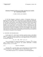
Definition 2.2. The bounding box of a set of points E is defined as the smallest axis-
parallel rectangle containing the set E in the graphical representation of the permuta tion
(see Figure 1). Thi s box defines several regions in the plane:
• The sides of the bounding box (U,L,R,D on Figure 1).
• The corners of th e bounding box (1, 2, 3, 4 on Figure 1).
• The boundin g box itself.
Figure 1 Graphical representation of σ = 12 13 11 3 1 7 10 2 9 8 5 6 4 and the bounding box
of {7, 2, 9, 5, 6}.
3
2 1
4
RL
D
U
Definition 2.3. A permutation π = π
1
. . . π
k
is called a pattern of the permutation σ =
σ
1
. . . σ
n
, with k ≤ n, if and only if there exist integers 1 ≤ i
1
< i
2
< . . . < i
k
≤ n such

that σ
i
ℓ
< σ
i
m
whenever π
ℓ
< π
m
. We will also say that σ contains π. A perm utation σ
that does not contain π as a pattern is said to avoid π.
Example 2.4. The permutation σ = 1 4 2 5 6 3 contains the pattern 1 3 4 2 whose
occurrences are 1 5 6 3, 1 4 6 3, 2 5 6 3 and 1 4 5 3. But σ avoids the pattern 3 2 1 as
none of its subsequences of length 3 is order-isomorphic to 3 2 1, i.e., is decreasing.
We write π ≺ σ to denote that π is a pattern of σ. This pattern-containment relation
is a pa rt ia l order on permutations, and permutation cla sses are downsets under this order.
In other words, a set C is a permuta tio n class if and only if for any σ ∈ C, if π ≺ σ, then
π ∈ C. Any class C of permutations can be defined by a set B of excluded patterns, which
is unique if chosen minimal (see for example [2, 10]), and which is called the bas is of C:
σ ∈ C if and only if σ avoids every pattern in B. The basis of a class of pattern-avoiding
permutations may be finite or infinite.
the electronic journal of combinatorics 18 (2011), #P57 3
Permutation classes have been widely studied in the literature, mainly from a pattern-
avoidance point of view. See [9, 23, 31, 39] among many others. The main enumerative
result about permutation classes is the proof of the Stanley-Wilf conjecture by Marcus
and Tardos [3 3], who established that for any class C, there is a constant c (the exponential
growth factor of C) such that the number of permutations of size n in C is at most c
n
.

Throughout this paper, we use the decomposition tree of permutations to characterize
pin-permutations. In these trees, permutations are decomposed along two different rules
in which two special kinds of permutations appear, the simple permutations and the linear
ones.
Strong intervals and simple permutations, whose definitions are r ecalled below, are the
two key co ncepts involved in substitution decompo sition. We refer the reader to [2, 3, 15 ]
for more details about simple permutations.
Definition 2.5. An interval or block in a permutation σ is a s et of consecutive integers
whose images by σ form a set of consecutive integers. A strong interval is an interval that
does not properly overlap
1
any other interval.
Definition 2.6. A permutation σ is simple when it is of size at least 4 and its non-empty
intervals are exactly the trivial ones: the singletons and σ.
Notice that the permutations 1, 12 and 21 also have only trivial intervals, nevertheless
they are no t considered to be simple here. Moreover no permutation of size 3 has only
trivial intervals.
Let σ be a permutation of S
n
and π
(1)
, . . . , π
(n)
be n permutations of S
p
1
, . . . , S
p
n
respectively. Define the substitution σ [π

(1)
, π
(2)
, . . . , π
(n)
] of π
(1)
, π
(2)
, . . . , π
(n)
in σ (also
called inflation in [2]) to be the permutation whose graphical representation is obtained
from the one of σ by replacing each point σ
i
by a block containing the graphical repre-
sentation of π
(i)
. More formally
σ[π
(1)
, π
(2)
, . . . , π
(n)
] = shift(π
(1)
, σ
1
) . . . shift(π

(k)
, σ
k
)
where shift(π
(i)
, σ
i
) = shift(π
(i)
, σ
i
)(1) . . . shift(π
(i)
, σ
i
)(p
i
) and
shift(π
(i)
, σ
i
)(x) = (π
(i)
(x) + p
σ
−1
(1)
+ . . . + p

σ
−1
(σ
i
−1)
) for any x between 1 and p
i
.
For example 1 3 2[2 1, 1 3 2, 1] = 2 1 4 6 5 3.
We have now all the basic concepts necessary to define deco mposition trees. For any
n ≥ 2, let I
n
be the permutation 1 2 . . . n and D
n
be n (n − 1) . . . 1. We use the
notations ⊕ and ⊖ for denoting respectively I
n
and D
n
, for any n ≥ 2. Notice that in in-
flations of the form ⊕[π
(1)
, π
(2)
, . . . , π
(n)
] = I
n
[π
(1)

, π
(2)
, . . . , π
(n)
] or ⊖[π
(1)
, π
(2)
, . . . , π
(n)
] =
D
n
[π
(1)
, π
(2)
, . . . , π
(n)
], the integer n is determined without ambiguity by the number of
permutations π
(i)
of the inflation.
Definition 2.7. A permutation σ is ⊕-indecomposable (resp. ⊖-indecomposable) if it
cannot be written as ⊕[π
(1)
, π
(2)
, . . . , π
(n)

] (resp . ⊖[π
(1)
, π
(2)
, . . . , π
(n)
]), for any n ≥ 2.
1
Two intervals I and J properly overlap when I ∩ J = ∅, I \ J = ∅ and J \ I = ∅.
the electronic journal of combinatorics 18 (2011), #P57 4
Theorem 2.8. (first appeared implicitly in [27]) Every permutation σ ∈ S
n
with n ≥ 2
can be uniquely decomposed as either:
• ⊕[π
(1)
, π
(2)
, . . . , π
(k)
], with π
(1)
, π
(2)
, . . . , π
(k)
⊕-indecomposable,
• ⊖[π
(1)
, π

(2)
, . . . , π
(k)
], with π
(1)
, π
(2)
, . . . , π
(k)
⊖-indecomposable,
• α[π
(1)
, . . . , π
(k)
] with α a simple permutation .
It is important for stating Theorem 2.8 that 12 and 21 are not co nsidered as simple
permutations. An equivalent version of this theorem, which includes 12 and 21 among
simple permutations, is given in [2]. Notice that the π
(i)
’s correspond to strong intervals in
the permutation σ, and are necessarily the maximal strong intervals of σ strictly included
in {1, 2, . . . , n}. Another important remark is that:
Remark 2.9. Any block of σ = α[π
(1)
, . . . , π
(k)
] (with α a simple permutation) is either
σ itsel f , or is included in one of the π
(i)
’s.

As an example of the result presented in Theorem 2.8, σ = 1 2 4 3 5 can be written
either as 1 2 3[1, 1, 2 1 3] or 1 2 3 4[1, 1, 2 1, 1] but in the first form, π
(3)
= 2 1 3 is not
⊕-indecomposable, thus we use the second decomposition. The decomposition theorem
2.8 can be applied recursively on each π
(i)
leading to a complete decomposition where
each permutation that appears is either I
k
, D
k
(denoted by ⊕, ⊖ respectively) or a simple
permutation.
Example 2.10. Let σ = 10 1 3 12 11 14 1 18 19 20 21 17 16 15 4 8 3 2 9 5 6 7. Its recursive
decomposition can be written as
3 1 4 2[⊕[1, ⊖[1, 1, 1], 1], 1, ⊖[⊕[1, 1, 1, 1], 1, 1, 1], 2 4 1 5 3[1, 1, ⊖[1, 1], 1, ⊕[1, 1, 1]]].
Figure 2 The substitution decomposition tree and the graphical representation
(with non-trivial strong intervals marked by rectangles) of the permutation σ =
10 13 12 11 14 1 18 19 20 21 17 16 15 4 8 3 2 9 5 6 7.
3 1 4 2
⊕
⊖
⊖
⊕
2 4 1 5 3
⊖ ⊕
the electronic journal of combinatorics 18 (2011), #P57 5
The substitution decomposition recursively applied to maximal strong intervals lea ds
to a tree representation of this decomposition where a substitution α[π

(1)
, . . . , π
(k)
] is
represented by a node labeled α with k ordered children representing the π
(i)
’s. In the
sequel we will say the child of a node V instead of the permutation corresponding to the
subtree rooted at a child of node V .
Definition 2.11. The substitution decomposition tree T of the permutation σ is the unique
labeled ordered tree encoding the substitution decomposition of σ, where each internal node
is either labeled by ⊕, ⊖ -thos e nodes are called linear- or by a simple permutation α -
prime nodes Ea ch node labeled by α has arity |α| and each subtree maps onto a strong
interval of σ.
Notice that in substitution decomposition trees, there are no edges between two nodes
labeled by ⊕, nor between two nodes labeled by ⊖, since the π
(i)
’s are ⊕-indecomposable
(resp. ⊖-indecomposable) in the first (resp. second) item of Theorem 2.8. See Figure 2
for an example.
Theorem 2.12. [2] Permutations are in one-to-one correspondence with substitution d e -
composition trees.
2.2 Pin representations: basic definitions
We will consider the subset of permutations having a pin representation. Pin representa-
tions were introduced in [16] in order to check whether a permutation class contains only
a finite number of simple permutations. Nevertheless, pin representations can be defined
without reference t o simple permutations.
A diagram is a set of points in the plane such that two po ints never lie on the same
row or the same column. Notice that the graphical representation of a permutation is a
diagram and that a diagra m is not always the graphical representation of a permutation

but is order-isomorphic to the graphical representation of a permutation -just delete blank
rows and columns from the diagram. In a diagram we say that a pin p separates the set
E from the set F when E and F lie on different sides from either a horizontal line going
through p or a vertical one.
Definition 2.13. Let σ ∈ S
n
be a permutation. A pin representation of σ is a sequence
of points (p
1
, . . . , p
n
) of the graphical representation of σ (covering all the points in it)
such that each point p
i
for i ≥ 3 satisfies both of the following conditions
• the externality condition: p
i
lies outside of the bounding box of {p
1
, . . . , p
i−1
}
•





either the separation condition: p
i

must separate p
i−1
from {p
1
, . . . , p
i−2
},
or the independence condition : p
i
is not on the sides of the bounding box
of {p
1
, . . . , p
i−1
}.
the electronic journal of combinatorics 18 (2011), #P57 6
Figure 3 A pin representation of permutation σ = 1 8 3 6 4 2 5 7. All pins p
3
, . . . , p
8
are
separating pins, except p
6
which is an independent pin.
p
6
p
7
p
1

p
3
p
2
p
5
p
4
p
8
We say that a pin satisfying the externality and the independence (resp. separation)
conditions is an in dependent (resp. separati ng) pin. An example of a pin representation
is given in Figure 3.
Pin representations in our sense are more restricted than pin sequences in the sense of
[16, 18]: a pin representation covers all the points of the permutation, whereas this is not
required for a pin sequence. This difference justifies tha t we use the word representation
instead of sequence. Nevertheless our proper pin representations coincide with the proper
pin sequences defined in [16].
Definition 2.14. Let σ ∈ S
n
be a permutation. A proper pin representation of σ is a
sequence of points (p
1
, p
2
, . . . , p
n
) of the graphical representation of σ such that each point
p
i

satisfies both the separation and the externality cond i tion s .
Not every permutation has a pin representation, see for example σ = 7 1 2 3 8 4 5 6. We
call pin-permutation a ny permutation that has a pin representation. The set of pin-
permutations is a permutation class (see Lemma 3.3). Pin-permutations correspond to
the permutations that can be encoded by pin words in the terminology of [16, 18]. In
that paper the authors conjecture the following result:
Conjecture 2.15. [18] The cla s s of pin-permutations has a rational generating function.
In the sequel we prove this conjecture and exhibit the generating function of pin-
permutations. We first study some properties of pin representations.
2.3 Some properties of pin representations
We first give general properties of pin representations and define sp ecial families of pin-
permutations.
Lemma 2.16. Let (p
1
, . . . , p
n
) be a pin representation of σ ∈ S
n
. If p
i
is an in dependent
pin, the n {p
1
, . . . , p
i−1
} is a block of σ.
Proof. Neither p
i
nor the pins p
j

where j > i separate {p
1
, . . . , p
i−1
}. The former comes
from the independence of p
i
and the latter from the definition of pin representations.
the electronic journal of combinatorics 18 (2011), #P57 7
Lemma 2.17. Let (p
1
, . . . , p
n
) be a pin representation of σ ∈ S
n
. Then for each i ∈
{2, . . . , n − 1}, i f there exists a point x on the sides of the bounding box of {p
1
, . . . , p
i
},
then it is unique and x = p
i+1
.
Proof. Consider the bounding box of {p
1
, p
2
, . . . , p
i

} and let x be a point on the sides of
this bounding box. Suppose without loss of generality that x is above the bounding box.
By definition of the b ounding box, and since it contains at least two points, x separates
{p
1
, . . . , p
i
} into two sets S
1
, S
2
= ∅. Now, there exists l ≥ i such that x = p
l+1
. Suppose
that l > i. The bounding box of {p
1
, . . . , p
l
} contains the one of { p
1
, . . . , p
i
} but does
not contain x, and thus x is still above it. Consequently, x = p
l+1
does not satisfy the
independence condition. It must then satisfy the separation condition, so that x separates
p
l
from p

1
, . . . , p
l−1
. But S
1
, S
2
⊂ {p
1
, . . . , p
l−1
} and x separates S
1
from S
2
leading to a
contradiction.
Any pin representation can be encoded into words on the alphabet {1, 2, 3, 4} ∪
{R, L, U, D} called pin words associated to the pin representa tion of the permutation
and defined below.
Definition 2.18. Let (p
1
, p
2
, . . . , p
n
) be a pin representation. For any k ≥ 2, the pin p
k+1
is encoded as follows.
• If it separates p

k
from the set {p
1
, p
2
, . . . , p
k−1
}, then it lies on one side of the
bounding box. And p
k+1
is encoded by L, R, U, D in the pin word depending o n its
position as shown in Figure 1.
• If it respects the externality and independence conditions and therein lies in one of
the quadrant 1, 2, 3, 4 defined in Fig ure 1, then thi s numeral encodes p
k+1
in the pin
word.
To encode p
1
and p
2
: choose an arbitrary origin p
0
in the plane such that it extends the
pin represen tation (p
1
, p
2
, . . . , p
n

) to a pin sequence (p
0
, p
1
, . . . , p
n
); then encode p
1
with
the numeral corresponding to the position of p
1
relative to p
0
and encode p
2
according to
its pos i tion relative to the bound i ng box of {p
0
, p
1
}.
Notice that because of the choice of the origin p
0
, a pin representation is not associated
with a unique pin word, but with at most 8 pin words (see Figure 4). The set of pin words
is the set of all encodings of pin-permutations. Some pin words associated with the pin
representation of σ = 1 8 3 6 4 2 5 7 given in Figure 3 are 11URD3UR, 3 RURD3UR, . . .
Definition 2.19. A pin word w = w
1
. . . w

n
is a strict pin word if and only if only w
1
is
a numeral.
Note that in a strict pin word w = w
1
. . . w
n
, for any 2 ≤ i ≤ n − 1, if w
i
∈ {L, R},
then w
i+1
∈ {U, D} and if w
i
∈ {U, D}, then w
i+1
∈ {L, R} .
A strict pin word is the encoding of a proper pin representa t ion. A proper pin rep-
resentation corresponds to several pin words among which some are strict, but not all of
them.
the electronic journal of combinatorics 18 (2011), #P57 8
Figure 4 The two letters in each cell indicate the first two letters of the pin word encoding
(p
1
, . . . , p
n
) when p
0

is taken in this cell.
p
1
p
2
11
41
4R
21
31
3R
2U
3U
p
2
p
1
1D
4D
1L
13
43
2L
23
33
The gra phical representations of permutations of size n are naturally gridded into n
2
cells. We define the distance dist between two cells c and c
′
as follows: dist(c, c

′
) = 0 if
and only if c = c
′
, and dist(c, c
′
) = min
c
′′
∈N (c
′
)
dist(c, c
′′
) + 1 where N (c
′
) denotes the set
of neighboring cells of c
′
, i.e., the cells that share an edge with c
′
.
Lemma 2.20. Let (p
1
, . . . , p
n
) be a proper pin representation of σ ∈ S
n
. Then, for 2 <
i < n, the pin p

i
is at a distance of ex actly 2 cells from the bounding box of {p
1
, . . . , p
i−1
}.
Proof. From Definition 2.14 of proper pin representations, for 2 ≤ i < n, p
i+1
separates p
i
from {p
1
, . . . , p
i−1
}, therefore p
i
is at a distance of at least 2 cells from the bounding box
of {p
1
, . . . , p
i−1
}. Moreover from Definition 2.14 again and Lemma 2.17, for 2 < i < n,
p
i
is on the sides of the bounding box of {p
1
, . . . , p
i−1
} and p
i+1

is the only point on the
sides of the bounding box of {p
1
, . . . , p
i
}. Thus, for 2 < i < n, p
i
is at distance exactly 2
cells from t he bounding box of {p
1
, . . . , p
i−1
}.
Lemma 2.21. Let p = (p
1
, . . . , p
n
) be a proper pin representation of σ ∈ S
n
. If the pin
p
i
is at a corner of the bounding box of {p
1
, . . . , p
j
} with j ≥ i, then i = 1 or 2.
Proof. If the pin p
i
is at a corner o f the bounding box of {p

1
, . . . , p
j
} for some j ≥ i,
then p
i
is not on the sides of the b ounding box of {p
1
, . . . , p
i−1
}. As p is a proper pin
representation, this happens only when i = 1 or 2.
2.4 Oscillations and quasi-oscillations
Amongst simple permutations some special ones, called oscillations and quasi-oscillations
in the sequel, play a key role in the characterization of substitution decomposition trees
associated with pin-permutations (see Theorem 3.1). No t ice that o scillations have been
introduced in [18] and are also known under the name of Gollan permutations in the
context of sorting by reversals [30].
Following [18], let us consider the infinite oscilla t ing sequence defined (on N \ {0, 2}
for regularity of the graphical representation) by ω = 4 1 6 3 8 5 . . . (2k + 2) (2k − 1) . .
Figure 5 shows the graphical representation of a prefix of ω.
Definition 2.22 (oscillation). An increasing oscillation of size n ≥ 4 is a simpl e permu-
tation of size n that is contained as a pattern in ω. The increasing osc i llations of smaller
the electronic journal of combinatorics 18 (2011), #P57 9
size are 1, 21, 231 and 312. A decreasing oscillation is the reverse
2
of an increasing
oscillation.
Figure 5 The infinite oscilla t ing sequence, an increasing oscillation of size 10 and a
decreasing oscillation of size 11, with a pin representation for each.

.
.
.
2 4 1 6 3 8 5 10 7 9 9 11 7 10 5 8 3 6 1 4 2
It is a simple matter to check that there are two increasing (resp. decreasing) oscilla-
tions of size n for any n ≥ 3. Notice also that three oscillations are both increasing and
decreasing, namely 1, 2 4 1 3 and 3 1 4 2.
The following lemmas state a few properties of oscillations that can be readily checked.
Lemma 2.23. Oscilla tion s are pin-permutations and any increasing (resp. decreasing )
oscillation has proper pin representations whose starting points can be chosen in the top
right or bottom left hand corner (resp. top left or bottom right hand corner).
Lemma 2.24. In any increasin g oscillation ξ of size n ≥ 4, the first (resp. last) three
elements form an occurrence of either the pattern 231 or the pattern 213 (resp. 132 or
312). In Table 1, these are referred to as the initial pattern and the terminal pattern of
ξ.
We further define another special family of permutations: the quasi-oscillations.
Definition 2.25 (quasi-oscillations). An increasing quasi-oscillation of size n ≥ 6 i s
obtained from a n increasing oscillation ξ of size n − 1 by the addition of either a minim al
element at the beginning of ξ or a maximal element at the e nd of ξ, followed by a flip of
an element of ξ according to the rules of Table 1. The element that is flipped is called the
outer point o f the quasi-oscillation. We also define the auxiliary substitution point to be
the point add ed to ξ, and the main substitution point according to Table 1.
3
Furthermore, for n = 4 or 5, there are two increasing quasi-oscillations of size n:
2 4 1 3, 3 1 4 2, 2 5 3 1 4 an d 4 1 3 5 2. Each of them has two possible choices for its main
and auxiliary substitution points. See Figure 6 for more details. We do no t define the
outer point of a quasi-oscillation of size less than 6.
Finally, a decreasing quasi-oscillation is the reverse o f an in creasing quasi-oscillation.
2
The reverse of σ = σ

1
σ
2
. . . σ
n
is σ
r
= σ
n
. . . σ
2
σ
1
3
The first line of Table 1 reads as: If a maxima l element is added to ξ, ξ starts (resp. ends) with a
pattern 231 (resp. 132), then the corresponding increasing quasi-oscillation β is obtained by flipping the
left-most point of ξ to the right-most (in β), and the main substitution point is the largest po int of ξ.
the electronic journal of combinatorics 18 (2011), #P57 10
Table 1 Flips and main substitution points in increasing quasi-oscillations.
Element Initial Terminal Flipped . . . which Main
inserted pattern of ξ pattern of ξ element . . . becomes substitution point
max 231 132 left-most right-most largest
max 231 312 left-most right-most right-most
max 213 132 smallest largest largest
max 213 312 smallest largest right-most
min 231 132 largest smallest left-most
min 231 312 right-most left-most left-most
min 213 132 largest smallest smallest
min 213 312 right-most left-most smallest
Figure 6 The graphical representations of the quasi-oscillations of size 4, 5 and 6. The

points marked M, A and O represent respectively the main substitution point, the aux-
iliary substitution point, and the outer point (when defined) of each quasi-oscillation.
Size Increasing quasi-oscillations Decreasing quasi-oscillations
4
2 4 1 3
A
M
2 4 1 3
M
A
2 4 1 3
M
A
2 4 1 3
M
A
3 1 4 2
M
A
3 1 4 2
M
A
3 1 4 2
M
A
3 1 4 2
M
A
5
2 5 3 1 4

M
A
2 5 3 1 4
M
A
2 5 3 1 4
M
A
2 5 3 1 4
M
A
4 1 3 5 2
M
A
4 1 3 5 2
M
A
4 1 3 5 2
M
A
4 1 3 5 2
M
A
6
2 6 4 1 3 5
M
A
O
2 4 6 3 1 5
M

A
O
3 6 2 4 1 5
M
A
O
2 6 3 5 1 4
M
A
O
4 1 5 3 6 2
M
A
O
5 1 4 2 6 3
M
A
O
5 3 1 4 6 2
M
A
O
5 1 3 6 4 2
M
A
O
The following properties of quasi-oscillations can be readily checked.
Lemma 2.26. There are four increasing (resp. decreasing) quasi-oscillations of any size
n ≥ 6. This also holds for n = 4 or 5 when oscillations are counted with a multiplicity
the electronic journal of combinatorics 18 (2011), #P57 11

equals to the number of pairs of main a nd auxiliary substitution points.
Lemma 2.27. Every quasi-oscillation is a simple pi n-permutation.
Proof. This is readily checked fo r size n = 4 or 5. The flips defining quasi-oscillations
are chosen in a way that enf orces simplicity. One pin representation of a quasi-oscillation
can b e obtained starting with its main substitution point, then reading the auxiliary
substitution point, and proceeding through the quasi-oscillation using separating pins at
any step, to finish with the outer point, when defined. See an example on Figure 7.
Figure 7 Two examples of quasi-oscillations of size 10 and 11. The points marked M,
A and O represent respectively the main and auxiliary substitution points, and the outer
point.
2 10 4 1 6 3 8 5 7 9
M
A
O
4 1 6 3 8 5 10 7 9 11 2
M
A
O
We can no tice that the direction (increasing or decreasing) of a quasi-oscillation of
size n ≥ 6 is the same direction that is defined by the alignment of M and A, its main
and auxiliary substitution points. Therefore, we can equivalently express the direction
of a quasi-oscillation as shown in Definition 2.28, which also allows us to generalize it to
quasi-oscillations of size 4 and 5.
Definition 2.28. A quasi-oscillation together with a choice of the main and auxiliary
substitution points is said to be increasing (resp. decreasing) when these points form an
occurrence of the pattern 12 (resp. 21).
3 Characterization of the de composition tre e
Permutations are in one-to-one correspondence with decomposition trees. In this section
we give some necessary and sufficient conditions on a decomposition tree for it to be
associated with a pin-permuta t io n through this correspondence.

Theorem 3.1. A permutation σ is a pin-permutation if and on l y if its substitution de -
composition tree T
σ
satisfies the following conditions:
(C
1
) any linear node la beled by ⊕ (resp. ⊖) in T
σ
has a t most on e child that is not an
increasing (resp. decreasing) oscillation .
the electronic journal of combinatorics 18 (2011), #P57 12
(C
2
) any prime node in T
σ
is labeled by a simple pin-permutation α and satisfies one of
the follow i ng properties:
– it has at most one child that is not a singleton; moreover the poi nt of α corre-
sponding to the non-trivial child (if it exists) is an active poin t of α.
– α is a n in creasing (resp.decreas i ng) quasi-oscillation, and the node has exactly
two children that are not singletons: one of them expands the main substitution
point of α a nd the other one is the permutation 12 (resp. 21), expanding the
auxiliary substitution point of α .
3.1 Preliminary remarks
Let σ be a pin-permutation. Then σ has pin representatio ns, but not every point of σ
can be the starting point for such a representation. Therefore we define:
Definition 3.2. An active point of a pin-permutation σ is a point that is the starting
point of some p i n representation of σ.
We now recall some basic pro perties of the set of pin-permutations.
Lemma 3.3 ([18]). The set of pin-permutations is a class o f permutations. Moreover, if

p is a pin representation for some permutation σ, then for any π ≺ σ, there exists a pin
representation of π obtained from p, by keeping in the same order points p
i
that form an
occurrence of π in σ.
Instead of random patterns of a pin-permutat io n σ, we will often be interested in
patterns defined by blocks of σ and state a restriction of Lemma 3.3 to t his case:
Corollary 3.4. If σ is a pin- permutation, then the permutation associated to every block
of σ is also a pin-permutation.
The following remark will be used many times in the next proofs:
Remark 3.5. Let σ be a pin-permutation wh ose substitution decomposition tree ha s a root
V , and B the block of σ corresponding to a given child of V . If in a pin representation
of σ there exist indices i < j < k with p
i
∈ B , p
j
∈ B , and p
k
is a pin separating p
i
from
p
j
, then p
k
also belongs to B.
Assume σ is a pin-permutation and consider nodes in the substitution decomposition
tree T
σ
of σ. They are roots of subtrees of T

σ
corresponding to permutat io ns that are
blocks of σ, and that are consequently pin-permutations. As a consequence, for finding
properties of the nodes in the subst itution decomposition tree of a pin-permut ation, it
is sufficient to study the properties of the roots of the substitution decomposition trees
of pin-permutations. Before attacking this problem, we introduce a definition useful to
describe the behavior of a pin representation of σ on the children of the root of T
σ
.
the electronic journal of combinatorics 18 (2011), #P57 13
Definition 3.6. Let σ be a pin-permutation and p = (p
1
, . . . , p
n
) be a pin repres e ntation
of σ. For an y set B of points of σ, if k is the number o f maximal factors p
i
, p
i+1
, . . . , p
i+j
of p th at contain only points o f B, we say that B is read in k times by p. In particular
B is read in one time by p when all points of B form a single segment of p.
Let σ be a pin-permutation whose substitution decomposition tree has a root V , and
p = (p
1
, . . . , p
n
) be a pin representation of σ. We say that some child B of V is the k- t h
child to be read by p i f, letting i be the minimal index such that p

i
belongs to B, the points
p
1
, . . . , p
i−1
belong to exactly k − 1 different chi l dren of V .
Mostly, we use Definition 3.6 on sets B that are blocks of σ, and even more precisely
children of the root of the substitution decomposition tree of σ.
3.2 Properties of linear nodes
We analyze first the structure of pin representations of any pin-permuta tion σ whose
substitution decomposition tree has a root that is a linear node V a nd give a precise
description of the children of V in Lemma 3.7.
Lemma 3.7. Let σ be a pin-permutation whose substitution decomposition tree has a
root that is a linear node V labeled by ⊕ (resp. by ⊖). Then at mos t one child of V is
not an ascending (resp . descending) oscillation, it is the first child that is read by a pin
representation of σ, and all other children are read in one time.
Proof. Assume that the node V has label ⊕, the other case being similar. Let T
1
, . . . , T
k
be the children of V , from left to right. Let p be a pin representation of σ. Denote by
T
i
0
the first child that is read by p. Let i be t he minimal index such that p
i
belongs
to T
ℓ+1

(for so me ℓ ≥ i
0
). Suppose p
i−1
as just been read by p. Then the points of
T
ℓ+1
are in the top right hand corner with respect to the points t hat have already been
read by p (including at least one point of T
i
0
). Therefore, they correspond to pins that
are encoded by a symbol 1, U or R in a pin word. Furthermore, the only point that is
encoded by the symbol 1 is the first point of T
ℓ+1
that is read by p. Indeed, because
T
ℓ
is ⊕-indecomposable, any other symbol 1 would mean that p star ts the reading of an
other child T
j
with j > ℓ + 1. Consequently, T
ℓ+1
is a permutatio n represented by a pin
word of t he form either 1URUR . . . or 1RURU . . ., tha t is to say, T
ℓ+1
is an ascending
oscillation. So from Lemma 2.17, T
ℓ+1
is read in one time by p. In the same way, we can

prove that any T
ℓ−1
with ℓ ≤ i
0
is a permutation encoded by a pin word of the form either
3LDLD . . . or 3DLDL . . ., or in other words, that T
ℓ−1
is again an ascending oscillation
and is read in one time by p. As a conclusion, the only child of V that might not be an
ascending oscillation is the first child that is read by a pin representation of σ, and all
other children are rea d in one time.
3.3 Properties of prime nod es
We analyze next the structure of pin representations of any pin-permutation σ whose
substitution decomposition tree has a root that is a prime node V . We will often use the
the electronic journal of combinatorics 18 (2011), #P57 14
following reformulation of Remark 2.9 (p.5) in t erms of substitution decomposition trees
in the proofs of this subsection.
Remark 3.8. Let σ be a permutation whose substitution decomposition tree has a root V
that is a prime node. There is no block in σ that intersects several children of V , except
σ itsel f .
We start with proving a technical lemma:
Lemma 3.9. Let σ be a pin-permutation whose substitution decomposition tree has a
root V that is a prime node, and let p = (p
1
, . . . , p
n
) be a pin representation of σ. If an
independent pin p
i
is the first point of a child B of V to be read by p, then B is either the

first or the second child of V that i s read by p.
Proof. Assume that B is the k-th child of V to be read by p, with k = 1, 2, and denote by
p
i
the first point of B that is read by p. Proving that p
i
satisfies the separation condition
(and theref ore does not satisfy the independence condition) will give the announced result.
Denote by C the (k − 1)-th child of V that is read by p, and by D the (k − 2)-th child of
V that is read by p. Since B is at least the third child of V that is read by p, C and D are
well defined. Now, if p
i
were an independent pin, then from Lemma 2.16 {p
1
, . . . , p
i−1
}
would form a block in σ intersecting more than one child of V (at least children C and D)
but not all of them (not B). This contradicts Remark 3.8 and concludes the proof.
Consider a pin-permutation σ whose substitution decomposition t r ee has a root V that
is a prime node. Lemma 3.11 is dedicated to the characterization of the restricted cases
where a child o f a prime node V can be r ead in more than one time (see Example 3.10).
Example 3.10. Let σ = 5 4 1 2 6 3 be the permutation whose substitution decomposition
tree is given in Figure 8. There exist two pin representations for σ depending on the order
of p
1
and p
2
, an d they both read the leftmost child of V in two tim es (see Figure 8).
Figure 8 The decomposition tree T

σ
and a pin representat io n p of σ = 5 4 1 2 6 3.
3 1 4 2
⊖
⊕
p
6
p
3
T
1
p
1
p
2
T
2
p
5
T
3
p
4
T
4
Lemma 3.11. Let σ be a pin-permutation whose substitution decomposition tree has a
prime node V as root and let p = (p
1
, . . . , p
n

) be a pin representation of σ.
(i) If some child B of V is read in more than one time by p, then it is read in exactly
two times, the second part being the last point p
n
of p.
the electronic journal of combinatorics 18 (2011), #P57 15
(ii) At most one of the children of V can be read in two times b y p and it is the first o r
the second child of V to be read by p.
Proof. We write the pin representation p as p = (p
1
, . . . , p
i
, . . . , p
j
, p
j+1
, . . . , p
k
, . . . , p
n
)
where p
i
is the first point of B that is read by p, all the pins from p
i
to p
j
are points of B,
p
j+1

does not belong to B, and p
k
is the first point belonging t o B after p
j+1
. These points
are well-defined since B is read by p in more than one time. To obtain the announced
result, we need to prove that k = n.
For k ≤ h ≤ n, p
h
is a separating pin. Otherwise p
h
would be an independent pin
and from Lemma 2.16 we would have a block p
1
, . . . , p
h−1
in σ intersecting more than one
child of V (na mely B and the block p
j+1
belongs to), contradicting Remark 3.8 since V
is prime. Moreover we can prove inductively that p
h
∈ B for k ≤ h ≤ n. This is true
for h = k. Consider h ∈ {k + 1, . . . , n}. By induction hypothesis, p
h−1
belongs to B. As
p
h
satisfies the separation condition, it separates p
h−1

from {p
i
, . . . , p
j
} ⊂ {p
1
, . . . , p
h−2
}
and therefore belongs to B from Remark 3.5. As a conclusion, all points p
k
, p
k+1
, . . . , p
n
are points of B.
Moreover at most one child of V is discovered before p
i
. Indeed it is the case when i ≤ 2
and when i ≥ 3, we prove that p
i
is an independent pin. Ot herwise p
i
separates p
i−1
from
{p
1
, . . . , p
i−2

} and therefore must all other points of B, contradicting Lemma 2.17. We
conclude with Lemma 3.9 that, since p
i
is the first point of B that is read, a t most one child
of V appears before B. Consequently since any simple permutatio n is of size at least 4 (see
p.4) and p can be decomposed as p = ( p
1
, . . . , p
i−1
  
at most one child
, p
i
, . . . , p
j
  
∈B
, p
j+1
, . . . , p
k−1
  
/∈B
, p
k
, . . . , p
n
  
∈B
),

there are, among p
j+1
, . . . , p
k−1
, some points belonging to at least two different children
of V , both different from B. Let us denote by C the child of V p
k−1
belongs to, and by D
another child of V that appears in p
j+1
, . . . , p
k−1
. As p
k
separates p
k−1
from the previous
pins, B (through p
k
) separa t es C (to which p
k−1
belongs) from D (to which some other
pin before p
k−1
belongs). But then any point of B that has not yet been read, namely
any point of {p
k
, . . . , p
n
}, is on the sides of t he bounding box of {p

1
, . . . , p
k−1
}. Since
from Lemma 2 .1 7 (p. 8) there is at most one point on the sides of this bounding box, we
conclude that k = n.
At that point, given a pin-permutation σ whose substitution decomposition tree T
σ
has a prime root, we know how a pin representation of σ proceeds through the children
of this root. In Lemma 3 .1 2 we tackle the problem of characterizing those children more
precisely.
Lemma 3.12. Let σ be a pin-permutation whose substitution decomposition tree has a
prime root V and p = (p
1
, . . . , p
n
) be a pin representation of σ.
(i) V has at most two children that are not singletons.
(ii) If there exists a child B of V that is not a singleton and that is not the first child
of V to be read by p then B contains e x actly two points, the first point of B read by
the electronic journal of combinatorics 18 (2011), #P57 16
p is an inde pende nt pin, the second one is p
n
. Moreover the first child of V read by
p is read in one time and B is the secon d child o f V read by p.
Proof. Suppose there exists a child B of V which is not a singleton, and such that B is
not the first child of V to be read by p. We denote by p
i
the first po int of B that is read
by p. By hypot hesis, i ≥ 2 and i = n.

Suppose that p
i
is a separating pin. Then necessarily, i ≥ 3 (it is impossible for p
i
to separate a set of less t han 2 points), and p
i
is on the sides of the bounding box of
{p
1
, . . . , p
i−1
}. But since p
i
is the first point of B that is read, any point of B is also
on the sides of this bounding box. With Lemma 2.17, this contradicts that B is not a
singleton. Consequently, p
i
is an independent pin.
By Lemma 3.9, and since we assumed it is not the first, B is the second child of V
to be read by p. Let us denote by C the first child of V that is read by p. Because V is
prime, there must be a point in σ, belonging to another child D of V , that separa t es child
B from child C of V . This po int separates in particular p
i
from p
1
, and it is necessarily
p
i+1
, since no pin after p
i+1

can separate p
1
from p
i
. This proves that p
i+1
/∈ B. With
Lemma 3.11(i), we get that either B = {p
i
} or B = {p
i
, p
n
}. Because B is not a singleton,
the latter holds.
Since B is read in two times, Lemma 3.11 ensures that t he first child of V is read in
one time by p.
Finally, the first child of V read by p may not be a singleton, but by the above, every
other child o f V that is not a singleton co ntains p
n
. Hence V has at most two children
that ar e not singletons.
3.4 Proof of Theorem 3.1: necessary condition
With the previous technical lemmas, we prove in this subsection that conditions (C
1
) and
(C
2
) of Theorem 3.1 (p.13) are necessary conditions on the substitution decomposition
tree T

σ
of σ for σ to be a pin-permutation.
Let σ be a pin-permutation whose substitution decomposition tree is T
σ
. Any node V
in T
σ
is the root of some subtree T of T
σ
. Moreover, T is the substitution decomposition
tree T
π
of some permutation π ≺ σ, and π is a pin-permutation by Corollary 3.4 (p.13).
Consequently, we only need to prove that:
• if V is a linear node, condition (C
1
) is satisfied by the r oot of T
π
,
• if V is a prime node, condition (C
2
) is satisfied by the root of T
π
.
When V is a linear node, we conclude thanks to Lemma 3 .7 (p.14).
So, let us assume that V is a prime node, labeled by a simple permutation α. With
Lemma 3.3 (p.13 ), it is immediate to prove that t he simple permutation α labeling node
V is a simple pin-permutation, since it is a pattern of π. By Lemma 3.12, V has at most
two children that are not singletons. If all children of V are singletons, condition (C
2

) is
satisfied.
the electronic journal of combinatorics 18 (2011), #P57 17
Assume V has exactly one child B t hat is not a singleton, and consider a pin r epre-
sentation p = (p
1
, . . . , p
n
) of π. We need to prove t hat this child expands an active point
of α. If B is the first child of V to be read by p, then π contains an occurrence of α in
which B is represented by the first point p
1
of p. Hence by L emma 3 .3 there exists a pin
representation for α whose first point, active for α by Definition 3.2, is the one represent-
ing B. When p does not start with reading B, we apply Lemma 3.12: B contains exactly
two points, the first one read in p is p
2
(read just after the first child read by p, which
is a singleton – hence p
1
– by hypot hesis) and the second one is p
n
. Observing that the
first two points in a pin representation play symmetric roles, it does not matter in which
order there are taken: a consequence is that (p
2
, p
1
, p
3

, . . . , p
n
) is another admissible pin
representation for π and an occurrence of α in π is composed of all points of p except p
n
.
Therefore (p
2
, p
1
, p
3
, . . . , p
n−1
) is a pin representa tion for α in which B is represented by
p
2
and thus B expands an active point of α.
Let us now assume that node V has exactly two children that are not singletons.
Lemma 3.12 shows that any pin representation p = {p
1
, . . . , p
n
} of π is composed as
follows:
• the first child of V to be read by p is one of the non-trivial children, denoted by C,
the other one denoted by B consisting of two points,
• C is read in one time by p,
• the first point of B read by p is an independent pin,
• the second and last point of B read by p is p

n
.
Without loss of g enerality (that is to say up to symmetry), we can assume that B is
in the top right hand corner with respect to C. This situation is represented on Figure 9.
Figure 9 Permutation π around its two non-trivial children B and C.
B
C
Bounding box
when p has read C
and the first point of B
acceptable
not acceptable
If the block B contains the permut ation 21, then the second p oint of B would be on the
sides of the bounding box when p has read C and the first point of B, and by L emma 2.17
the electronic journal of combinatorics 18 (2011), #P57 18
(p.8) this second point of B would have to be read just a fter the first one contradicting the
primality of V (since a prime node has at least four children). Consequently, B contains
the permutation 12.
Between the two points of B, p r eads all the points of π that corresp ond to trivial
children of V . Because V is prime, from Lemma 2.16 (p.7) and Remark 3.8 (p.15) all of
these points are separating pins and there are at least two of them. There are four possible
positions for the first such pin that is read by p, but only two of them ar e acceptable since
we need α to be simple. Indeed, choosing the up or right pin on Figure 9 (pins that are
indicated as not acceptable) would imply that the seco nd point of B is on the sides of
the bounding box, so it has to be taken now, and since it is the last point of p, the pin
representation stops, contradicting as before the primality of V . Therefore we can assume
that the first pin after the first point of B is the one in the top left hand corner of C, the
other possible one leading to a symmetric configuration. The pin representation is then
an alternation of down and left pins, until p
n−1

which is an up or right pin.
Consequently there is only one possible way of putting the pins corresponding to the
trivial children of V that does not contradict that α is simple, nor that B conta ins two
points. This only possible configuration is represented on Figure 10, and it corresponds to
the case in which α is a quasi-o scillation, with C expanding its main substitution point,
and B expanding its auxiliary substitution point. Moreover, if the quasi-oscillation is
increasing (resp. decreasing), then B contains the permutation 12 (resp. 21). The reason
is that, by Definition 2.28, the direction defined by the alignment of blocks B and C is
the same a s the direction of the quasi-oscillation.
Figure 10 The only configuration (up to symmetry) of a pin-permutation whose root is
a prime node with two non trivial children.
B
p
n
C
·
·
·
p
n−2
p
n−1
This concludes the proof that conditions (C
1
) and (C
2
) are necessary conditions on a
permutation σ for σ to be a pin-permutation.
3.5 Proof of Theorem 3.1: suffic ient condition
We can now end the proof of Theorem 3.1 by proving that conditions (C

1
) and (C
2
) are
sufficient for a permutation σ to be a pin-permutation. In the following we prove by
the electronic journal of combinatorics 18 (2011), #P57 19
induction on the size of σ that a permutation satisfying conditions (C
1
) and (C
2
) is a
pin-permutation. Recall that T
σ
denotes the substitution decomposition tree of σ. Notice
that for σ = 1, conditions (C
1
) and (C
2
) are vacuously true. The pin representation
with only one pin is a pin representation for σ. Assume now that |σ| > 1, and that any
permutation π such that |π| < |σ| satisfying conditions (C
1
) and (C
2
) is a pin-permutation.
We distinguish two cases, a ccording to the type (linear or prime) of the root of T
σ
.
When the root of T
σ

is a linear node, consider σ = ⊕[σ
(1)
, σ
(2)
, . . . , σ
(k)
], without loss of
generality, and assume that σ satisfies (C
1
) and (C
2
). Since the decomposition trees o f the
(σ
(i)
)
1≤i≤k
are subtrees of T
σ
, we get that the (σ
(i)
)
1≤i≤k
also satisfy conditions (C
1
) and
(C
2
). We can use the induction hypo t hesis on the (σ
(i)
)

1≤i≤k
, and obtain that they are all
pin-permutations. Moreover, condition (C
1
) holds fo r the root of T
σ
, and we deduce that
at most one of the (σ
(i)
)
1≤i≤k
is not an increasing oscillation. We define i
0
as the index
such that σ
(i
0
)
is not an increasing oscillation, if it exists. Otherwise, we can pick any
integer i
0
∈ [1 k]. Since σ
(i
0
)
is a pin-permutation, it admits a pin r epresentation p
(i
0
)
.

By Lemma 2.2 3 (p.10), for any i < i
0
(resp. any i > i
0
), there exist pin representations
p
(i)
of σ
(i)
(which is an increasing oscillation) whose origin is in the top right hand corner
(resp. in the bottom left hand corner). Now p = p
(i
0
)
p
(i
0
−1)
. . . p
(1)
p
(i
0
+1)
. . . p
(k)
is a pin
representation for σ, proving that σ is a pin-permutation. We can remark that many
other pin representatio ns p for σ could have been defined from the (p
(i)

)
1≤i≤k
. Namely,
p = p
(i
0
)
w with w any shuffle o f p
(i
0
−1)
. . . p
(1)
and p
(i
0
+1)
. . . p
(k)
is suitable.
When the root of T
σ
is a prime node, consider σ = α[σ
(1)
, σ
(2)
, . . . , σ
(k)
] for a simple
permutation α, and assume that σ satisfies (C

1
) and (C
2
). As before, by induction
hypothesis, the (σ
(i)
)
1≤i≤k
are all pin-permutations. We denote by p
(i)
a pin representation
of σ
(i)
. Recall that every permuta t io n σ
(i)
expands the point α
i
of α. Applying condition
(C
2
) to the root of T
σ
, we also get that α is a pin-permutation. By condition (C
2
), at
most two permuta t io ns among σ
(1)
, σ
(2)
, . . . , σ

(k)
are not singletons.
When all permutations σ
(1)
, σ
(2)
, . . . , σ
(k)
are trivial , then σ = α, implying that σ is
a pin-permutat io n. When σ
(i)
is the only permutation that is not a singleton, then by
condition (C
2
) σ
(i)
expands an active point of α. Thus, there exists a pin representation
p of α with p
1
= α
i
. To get a pin representation for σ, we replace p
1
in p with the pin
representation p
(i)
of σ
(i)
. By exhibiting a pin representation for σ, we proved that σ is a
pin-permutation.

When two permutations among σ
(1)
, σ
(2)
, . . . , σ
(k)
are not trivial, then without loss of
generality α is an increasing quasi-oscillation, and among the two children that are not
singletons, one (say σ
(i)
) expands the main substitution point α
i
of α and the other one
(say σ
(j)
) is the permuta t io n 12, expanding the auxiliary substitution point α
j
of α. Let
p be the pin representation of α with p
1
corresponding to the main substitution point
and p
2
to the auxiliary one. In order to get a pin representation for σ, we first remove
the first pin of p a nd replace it by the pin representation p
(i)
of σ
(i)
. Then replace p
2

with the point of σ
(j)
that is closest to the block σ
(i)
. Beca use the two points expanding
α
j
follow the direction defined by the alignment of the main and auxiliary substitution
points of α, we can define the notion of the point of σ
(j)
closest to the block expanding
the main substitution point of α. Proceed reading all following points in p and finally
the electronic journal of combinatorics 18 (2011), #P57 20
read the second point of σ
(j)
, which separates the last point read in p (the outer point
when |α| ≥ 6) from all the previous ones.
This finally gives a pin representation for σ, showing that σ is a pin-permutation and
thus ending the proof that conditions (C
1
) and (C
2
) are sufficient for a permutation to be
a pin-permutation.
In Section 5, we compute the generating function for the class of pin-permutations,
proving that it is rational. The proof is based on the characterization of the decompo-
sition t rees of the pin-p ermutations, given in Theorem 3.1, and it uses standard t ools in
enumerative combinatorics [24]. However, it requires to compute as a starting point the
generating function of the simple pin-permutations. Section 4 is dedicated to this goal.
4 Generating function of the simple pin-per mut ations

We introduce some more terminology here.
Definition 4.1. A pin representation p = (p
1
, p
2
, . . . , p
n
) is sai d to be a simple pin
representation and a pin w ord w = w
1
w
2
. . . w
n
is said to be a simple pin word if the
permutation σ they encode is simple.
Notice that a simple pin representation is always a proper pin representation (see
Definition 2.14 and Lemma 2.16). However, not every proper pin representation (or strict
pin word) encodes a simple pin-permutation.
We shall be interested in chara cterizing the simple pin representations for enumerat-
ing them, in order to g et the generating function o f the simple pin-permutations. The
enumeration of simple pin representatio ns will be done in Subsection 4.2. Although there
is not a one-to-one correspondence between simple pin representations and simple pin-
permutations, we can compute how many simple pin representations are associated with
a single simple pin-permutation. This will allow us to derive the enumeration of simple
pin-permutations from the one of simple pin representations in Subsection 4.3.
Before this, we start with important properties of the first two points of every proper
pin representation. This is presented in Subsection 4.1, together with relatio ns between
strict pin words a nd pr oper pin representations (see Definitions 2.1 4 and 2.19).
4.1 Beginning of a pin representation of a simple pin-permutation

Definition 4.2. Let σ be a permutation gi ven by its graphical representation. We say
that two points x and y of σ are (or that the pair of points (x, y) is) in knight position
when the distance between the points x and y is exactly 3 cells and the two points are
neither on the same row nor on the same column (see Figure 11).
Lemma 4.3. Le t p = (p
1
, p
2
, . . . , p
n
) denote a proper pin representation of s ome permu-
tation σ. If |σ| > 2 the first two pins p
1
, p
2
are i n knight position.
the electronic journal of combinatorics 18 (2011), #P57 21
Figure 11 Knight position between two points.
Proof. By definition of proper pin representations, and since |σ| > 2, p
3
separates p
2
from
p
1
, and no other future pin separates p
2
from p
1
. Thus p

1
and p
2
are only be separated
by p
3
. This proves that p
1
and p
2
are in knight position.
Lemma 4.4. Let σ be a simple pin-permutation and p = (p
1
, p
2
, . . . , p
n
) be one of its
simple pin representations. If two points p
i
and p
j
of σ are in knight position then {i, j}∩
{1, 2, n} = ∅.
Proof. First recall that as σ is simple, by Lemma 2.16 (p.7) every pin p
i
(i ≥ 3) separates
p
i−1
from {p

1
, . . . , p
i−2
}. Consider the pin p
i
. We will be looking for all t he points p
j
,
with j < i, such that (p
i
, p
j
) are in knight position in σ. We want to prove that for each
such j, {i, j} ∩ {1, 2, n} = ∅. Assume i ≥ 3 and i < n, t he claim being obviously true
for i = 1 or 2 o r n. Without loss of generality, we suppose that p
i
separates the previous
pins from above as shown in Figure 12 and that p
i−1
lies on the right of p
i
. The thick
rectangle represents the bounding box of {p
1
, . . . , p
i−1
}.
Figure 12 Pin representations where i < n in the proo f of Lemma 4.4 .
c
′

c
p
i−1
p
i
p
i+1
Since i < n, p
i+1
separates p
i
from the previous pins, from the left or the right as
shown in Fig ure 12. Thus p
i
could only be in knight position with a previous pin p
j
in
one of the two gray cells c and c
′
.
There is a pin in c
′
: Only p
i−1
can be in c
′
and in that case it means that p
i−1
is
either p

1
or p
2
otherwise from Lemma 2.21 it could not be a t a corner of the bounding
box. Thus, there could be a pair of pins in knight positions between (p
1
, p
2
) or (p
2
, p
3
).
There is a pin in c: The pin in c must be p
1
or p
2
, otherwise it would separate vertically
two previous pins, o ne on its left and o ne on its right, inside the bounding box and the
only pin on its right is p
i−1
. Thus there could be a pair of pins in knight position between
p
i
and the pin in c, namely p
1
or p
2
.
In all cases, {i, j} ∩ {1, 2, n} = ∅.

Definition 4.5. An active knight in a pin-permutation σ i s an unordered pair of points
(x, y) in knight position that can be the first two poi nts of a pin representation of σ.
the electronic journal of combinatorics 18 (2011), #P57 22
As a consequence of Lemma 4.3 the number of pin representations of a simple pin-
permutation depends on its number of active knights.
Lemma 4.6. In any simple pin-permutation σ , there are at most two active knights
except f or the four permutations : 3 1 4 2, 2 4 1 3, 2 5 3 1 4 and 4 1 3 5 2 which have four
active knights. The simple pin-permutations of size at m o st 6 and their a ctive kn i ghts are
represented o n Table 2.
Table 2 The simple pin-permutations of size n ≤ 6 and t heir active knights.
n 1 active knight 2 a ctive knights 4 active knights
4
2 4 1 3 3 1 4 2
5
2 4 1 5 3 3 1 5 2 4 3 5 1 4 2 4 2 5 1 3 2 5 3 1 4 4 1 3 5 2
6
2 5 1 4 6 3 2 5 3 1 6 4 2 5 3 6 1 4
2 6 4 1 5 3 3 1 6 4 2 5 3 5 1 4 6 2
3 6 1 4 2 5 3 6 4 1 5 2 4 1 3 6 2 5
4 1 6 3 5 2 4 2 6 3 1 5 4 6 1 3 5 2
5 1 3 6 2 4 5 2 4 1 6 3 5 2 4 6 1 3
5 2 6 3 1 4
2 4 1 6 3 5 2 4 6 3 1 5 2 5 1 3 6 4
2 6 3 5 1 4 2 6 4 1 3 5 3 1 4 6 2 5
3 1 5 2 6 4 3 6 2 4 1 5 4 1 5 3 6 2
4 6 2 5 1 3 4 6 3 1 5 2 5 1 3 6 4 2
5 1 4 2 6 3 5 2 6 4 1 3 5 3 1 4 6 2
5 3 6 1 4 2
For each n > 6, all simpl e pin - permutations of siz e n have exactly one active knight,
except twelve of them that have two active knights, and that are:

• the four oscillations of size n,
• the eight quasi-oscillations of size n.
the electronic journal of combinatorics 18 (2011), #P57 23
Proof. The results presented in Table 2 can be obtained by exhaustive examination.
Let σ be a simple pin-permutation of size n > 6 and let p = (p
1
, p
2
, . . . , p
n
) be a pin
representation of σ. By Lemma 4.3, the pair of points (p
1
, p
2
) is an active knight of σ. We
want to prove that every permutation with at least two active knights is an oscillation or
a quasi-oscillation. It can be easily checked that oscillations and quasi-oscillations have
exactly two active knights. Assume σ has more than one active knight, one of them being
(p
1
, p
2
). By Lemma 4.4 the second active knight could be either (p
1
, p
i
), (p
2
, p

i
) or (p
i
, p
n
),
for some i.
The second active knight is (p
1
, p
i
). Without loss of generality, consider p
1
and p
2
in
relative positions shown in Figure 13. Then there are seven different possible positions
for a point p
i
to be in knight position with p
1
as shown in the figure. Po sitions 7 and 3
are in conflict (same row or same column) with point p
2
. A pin in position 1 creates an
interval with p
2
, which is impossible since σ is simple. Thus the only remaining possible
positions for p
i

are 2, 4, 5 and 6.
Figure 13 Knights between (p
1
, p
2
) and (p
1
, p
i
).
p
1
p
2
2
4
1
7
3
56
• the pin p
i
is in 5: Let r be a pin representation associated with σ but which begins
with (p
1
, p
i
). (This pin representation exists as (p
1
, p

i
) = (r
1
, r
2
) is an active knight.)
Then r
3
lies on t he row between r
1
and r
2
. By Lemma 2.20, r
3
is at distance 2 of
the bounding box of {r
1
, r
2
}. It cannot lies to the left of it as it would be in the
same column as p
2
. Thus r
3
is on the right side as shown in Figure 14. For the
same reason p
3
lies below the bounding box of {p
1
, p

2
} as shown in the first schema
of Figure 14.
Then p
4
has two different possible positions. It lies in the row separating p
2
from p
3
,
at distance 2 of the bo unding box of {p
1
, p
2
, p
3
} but is either on the right or on the
left of it (see Figure 14). If it lies on the right then the six points {p
1
, p
2
, p
3
, p
4
, p
i
, r
3
}

form a permutation of size 6, or an interval. This contradicts that σ is simple and
n > 6. So p
4
lies on the left. Then we can build a pin representation by alternating
left and down pins until we put a right or a up pin. It cannot be an up pin as
it will not respect the distance 2 condition with the bounding box of the previous
points (otherwise it would be in the same row as p
i
). If it is a r ig ht pin, it lies in
the column separating p
i
= r
2
from r
3
and thus is r
4
. But in that case, reading
the pin r epresentation r, r
4
is not at distance 2 of the bounding box of {r
1
, r
2
, r
3
}
contradicting Lemma 2.20.
• the pin p
i

is in 4: By similar arguments, it implies that the permutation is of size
strictly less than 6.
the electronic journal of combinatorics 18 (2011), #P57 24
Figure 14 Different cases for active knight (p
1
, p
i
).
p
2
p
1
p
i
r
3
p
3
p
4
p
4
p
2
p
3
p
1
p
i

• the pin p
i
is in 2: p
3
lies in the column between p
1
and p
2
at distance two of the
bounding box of {p
1
, p
2
}. It cannot lie below this bounding box as it would form
an interval with p
1
, p
2
, p
i
. Therefore it is above as shown in the second schema of
Figure 14. Then t here could be a pin representation made of alternating lef t and
up pins until we have a right or down one at position k. But then, p
i
separates this
pin from the preceding ones a nd must be p
k+1
. At that stage, {p
1
, . . . , p

k+1
} forms
an interval, and thus i = k + 1 = n. In that case we have a simple permutation with
two active knights, which is actually a quasi-oscillation.
• the pin p
i
is in 6: Then again σ is a quasi-oscillation.
The second active knigh t is (p
2
, p
i
). Considering that (p
2
, p
1
, p
3
, . . . , p
n
) is another pin
representation for σ, this case has already been solved by the previous one.
The second active knight is (p
i
, p
n
). Assume first that i ≥ 4. Consider then the
bounding box of {p
1
, . . . , p
i−2

}. Without loss of generality suppose that p
i−1
is above this
bounding box and that p
i
is a right pin as shown in Fig ure 15. Notice that since p
i−1
Figure 15 Case for active knight (p
i
, p
n
), i ≥ 4.
p
1
, . . . , p
i−2
p
i−1
p
i
1 2
3
4
56
7
8
is an up pin, in the b ounding box of {p
1
, . . . , p
i−2

} there is a point in every row and in
every column, except in the column of p
i−1
. As p
n
and p
i
form an active knight, p
n
must
be in one of the 8 positions drawn in the figure. But positions 3, 4, 5, 6 , 8 are forbidden
as another point lies in the same row. Position 7 is also forbidden for p
n
since it is inside
the bounding box of {p
1
, . . . , p
i−2
}. If p
n
is in position 2, then it means that the pin
representation r, which begins the reading of σ by r
1
= p
i
, r
2
= p
n
, then proceeds with

r
3
= p
i−1
and therefore p
i−1
must lie at distance 2 of the bounding box o f {p
i
, p
n
} i.e.
in the r ig htmost column of the bo unding box of {p
1
, . . . , p
i−2
} which is impo ssible. So
the electronic journal of combinatorics 18 (2011), #P57 25