Báo cáo toán học: "Relating different cycle spaces of the same infinite graph" docx
Bạn đang xem bản rút gọn của tài liệu. Xem và tải ngay bản đầy đủ của tài liệu tại đây (183.07 KB, 12 trang )
Relating different cycle spaces
of the same infinite graph
R. Bruce Richter and Brendan Rooney
Submitted: Jul 5, 2009; Accepted: Jun 11, 2001; Published: Jun 21, 2011
Mathematics Subject Classificiation: 05C10
Abstract
Casteels and Richter have shown that if X and Y are distinct compactifications
of a locally finite graph G and f : X → Y is a continuous surjection such that f
restricts to a homeomorphism on G, then the cycle space Z
X
of X is contained in
the cycle space Z
Y
of Y . In this work, we show how to extend a basis for Z
X
to a
basis of Z
Y
.
1 Introduction
Bonnington and Richter [1] introduced the cycle space of a locally finite graph as the edge
sets of subgraphs in which every vertex has even degree. Diestel and K¨uhn [4] introduced
a different cycle space for a locally finite graph G as the space “generated” by embeddings
of circles into the Freudenthal compactification F(G) of G. (The space F(G) is obtained
from G by adding one “point at infinity” for each “end” of G.)
Vella and Richter [7] unified these notions by introducing edge spaces and showing that
a nice cycle space theory holds for compact, weakly Hausdorff edge spaces (for definitions
see Section 2). In particular, the cycle space of Bonnington and Richter can be viewed as
the Diestel-K¨uhn cycle space, but in Alexandroff’s 1-point compactification A(G) of the
locally finite graph G, rather than in F(G).
Our first principal result clarifies the relation between the cycle spaces of a given edge
space, and its image under a continuous edge-preserving map. In particular, we show
how to use spanning trees to extend a basis of the smaller space to a basis of the larger
space. This recalls the fact that a basis of the cycle space of a given finite graph G can be
extended to a basis of the cycle space of any graph G
resulting from a sequence of vertex
identifications of G.
In order to better comprehend the statement, loosely speaking an edge space (X, E)
consists of a topological space X with a specified set E of disjoint open arcs (each arc
also an op en set in X), Z
(X,E)
denotes the cycle space of (X, E) (its elements are subsets
of E), and, relative to an analogue T of a spanning tree for (X, E), for each e ∈ E \ T ,
C
T
(e) is the fundamental cycle contained in T ∪ e.
the electronic journal of combinatorics 18 (2011), #P135 1
Theorem 1.1 Let (X, E) and (Y, E) be compact, connected, weakly Hausdorff edge spaces
and let f : X → Y be a continuous surjection so that, for each e ∈ E, f(e) = e and
f(X \ E) = Y \ E. Let T
Y
be the edge set of a spanning tree of (Y, E). Let T
X
be
the edge set of a spanning tree of (X, E) for which T
Y
⊆ T
X
and let z be in Z
(Y,E)
.
Then there exist unique z
∈ Z
(X,E)
and, for each e ∈ T
X
\ T
Y
, α
e
∈ {0, 1} so that
z = z
+
e∈T
X
\T
Y
α
e
C
T
Y
(e).
A main result in [1] considers a locally finite graph G embedded in the sphere with
a finite number of accumulation points. If there are k + 1 accumulation points, then the
face boundaries generate a subspace of the cycle space of A(G) having index k. Our other
principal result generalizes this fact. If the graph G can be embedded in the sphere with
k + 1 accumulation points, p e rforming k identifications converts the closure of the graph
into A(G). The theorem below treats the abstract case of a single identification, while
the corollary, proved by a trivial induction from the theorem, provides the case of finitely
many identifications.
Theorem 1.2 Let (X, E) be a compact, connected, weakly Hausdorff edge space such that
X \ E is totally disconnected. Let x, y ∈ X \ E be distinct and let Y be the quotient space
obtained from X by identifying x and y. Let P be the edge set of an xy-path in X. Then
P ∈ Z
(Y,E)
\ Z
(X,E)
and, for each z ∈ Z
(Y,E)
\ Z
(X,E)
, there is a unique element z
∈ Z
(X,E)
so that z = z
+ P .
Corollary 1.3 Let (X, E) be a compact, connected, weakly Hausdorff edge space such
that X \ E is totally disconnected. For i = 1, 2, . . . , k, let {x
i
, x
i
} be pairs of elements
of X \ E so that, for any nonempty subset I of {1, 2, . . . , k}, | ∪
i∈I
{x
i
, x
i
}| > |I|. Let
Y be the quotient space obtained from X by identifying x
i
with x
i
, i = 1, 2, . . . , k. For
each i = 1, 2, . . . , k, let P
i
be an x
i
x
i
-path in X. If z ∈ Z
(Y,E)
, then there exist unique
z
∈ Z
(X,E)
and, for i = 1, 2, . . . , k, α
i
∈ {0, 1} so that z = z
+
k
i=1
α
i
P
i
.
We remark that Theorem 1.2 and Corollary 1.3 apply in particular to the case of
distinct compactifications of a graph G; we are also motivated by other spaces. This
point is discussed in Section 3. All of the relevant definitions and preliminary results can
be found in Section 2. Section 4 has the proof of Theorem 1.1, while The orem 1.2 is
proved in Section 6. Section 5 is devoted to a deeper understanding of cycles that is used
in Section 6.
2 Preliminaries/Definitions
In this section, we provide the background material to place our work in context. We
believe there is merit to treating our infinite spaces more combinatorially than would be
usual in topology. Thus, we prefer edges to be open singletons, rather than real intervals.
In many places in this work, the vertex set will consist of closed singletons making a totally
disconnected subspace — this setting provides a very natural, simultaneous generalization
the electronic journal of combinatorics 18 (2011), #P135 2
of finite and infinite graphs, as well as the Freudenthal compactification (defined below)
of a locally finite graph.
An edge space is an ordered pair (X, E) consisting of a topological space X and a
subset E of X, called the edges, so that each e ∈ E is an open singleton whose boundary
has at most two elements. We refer to the points in the boundary of e as the nodes of e
and, if v is a node of e, then we say that v and e are incident. The motivation for edge
spaces is to generalize a natural topology of a graph. Let G be a graph with vertex set
V and edge set E. In the classical topology [7], the basic open sets are: for each e ∈ E,
{e}; and, for each v ∈ V , v plus all its incident edges. With this topology, topological
and graph-theoretic connection coincide. Among other things, we will be interested in
compactifications of G, which, for infinite graphs, means adding some additional points
and open sets corresponding to the “ends” of G.
An end of a graph G consists of an equivalence class of rays: two rays R and S are
equivalent if, for every finite set W of vertices, R and S have their tails in the same
component of G − W . A basic neighbourhood of the end ω is the component K of
G − W containing the tails of the rays in ω, plus all edges between K and W – but
not their incident vertices from W – and all the other ends whose rays’ tails lie in K.
The Freudenthal compactification F(G) of G is obtained by adding a new point for each
end, together with the basic neighbourhoods for each end. If G is locally finite, then
F(G) is compact. (More generally, if the deletion of any finite set of vertices leaves only
finitely many components, then F(G) is compact.) A compactification of G is any space
obtained by partitioning the end set of G into closed sets, and identifying the points in
F(G) corresponding to each part.
Since most topology texts generally assume all singletons are closed for their more
advanced theorems, at this stage it is necessary to develop the topological results more
suited to our context. This leads us to the following natural extension of the Hausdorff
property. A space X is weakly Hausdorff if for all x, y ∈ X there exist open sets U
x
and
U
y
so that: x ∈ U
x
; y ∈ U
y
; and |U
x
∩ U
y
| is finite. In the classical topology on a graph,
the only pairs that have no disjoint neighbourhoods are adjacent vertices, and a vertex
with an incide nt edge.
A cycle in an edge space (X, E) is a connected subspace Y of X so that: Y ∩ E is
not empty; for every e ∈ Y ∩ E, Y \ {e} is connected; and, for any distinct e, f ∈ Y ∩ E,
Y \ {e, f} is not connected. This definition should be compared with the “embedding of a
circle” definition of Diestel and K¨uhn. In Section 5, we clarify the relation between these
two definitions.
The cycle space Z
(X,E)
of (X, E) is the smallest subset of the power set 2
E
of E that
contains all the (edge-sets of) cycles and is closed under thin sums: a set C ⊆ 2
E
is thin
if each element of E occurs in only finitely many elements of C and the “sum” is the set
of elements of E that are in an odd number of elements of C.
We assume the reader is familiar with the following results from [7].
Lemma 2.1 Let (X, E) be a compact, weakly Hausdorff edge space.
1. There is a minimal connected subset T of X containing X \ E.
the electronic journal of combinatorics 18 (2011), #P135 3
2. Each edge e in E \ T is in a unique cycle, with edge set C
T
(e), contained in (E ∩
T ) ∪ {e}.
3. The set C = {C
T
(e) | e ∈ E \ T } is thin and, for every element z of Z
(X,E)
,
z =
e∈z\T
C
T
(e).
The minimal connected set T from Lemma 2.1 (1) is defined to be a spanning tree of
(X, E) (note that if X \ E is not totally disconnected, then T may not resemble a tree).
The elements C
T
(e) of C in (3) are defined to be the fundamental cycles (with respect to
T ). We shall also make use of the following results from Casteels and Richter [2].
Lemma 2.2 Let (X, E) and (Y, F ) be compact, weakly Hausdorff edge spaces and let f :
X → Y be a continuous surjection so that f : E → F is a bijection and f(X \E) = Y \F.
Then:
1. for any spanning tree T
Y
of (Y, F), there is a spanning tree T
X
of (X, E) containing
f
−1
(T
Y
); and
2. identifying each e ∈ E with f(e), Z
(X,E)
⊆ Z
(Y,F )
.
Our first result, Theorem 1.1, further clarifies the relationship Z
(X,E)
⊆ Z
(Y,F )
of
Lemma 2.2 by showing (perhaps as expected) that the basis {C
T
X
(e) : e ∈ E \ T
X
} of
Z
(X,E)
can be extended to a basis of Z
(Y,F )
by adding precisely the fundamental cycles
C
T
Y
(f(e)), for e ∈ E ∩ T
X
\ f
−1
(T
Y
).
3 Examples
In this section, we show that the hypotheses of Theorem 1.2 and Corollary 1.3 hold in
cases of interest.
As a simple example, consider the 2-way infinite ladder L (see Figure 1). Let a be the
end of L to the left and b the end to the right. Then F(L) is L plus these two additional
points. Let L
a=b
denote the space obtained from F(L) by identifying a and b (this is
the 1-point compactification A(L) of L). Let v and w be any two vertices of L. We can
set L
a=v
to be the space obtained by identifying a with v, L
b=w
the space obtained from
F(L) by identifying b with w, and L
a=v,b=w
the space obtained from L
a=v
by identifying b
with w. We emphasize that the compact spaces L
a=v
and L
b=w
are not compactifications
of L. However, they are compact spaces containing (although not homeomorphically)
the original graph and illustrate the notion of vertex identification. They are “graph-like
continuua,” defined below.
All these spaces have cycle spaces, which we naturally denote by Z
F
, Z
a=b
, Z
a=v
, Z
b=w
,
and Z
a=v,b=w
. All of these contain Z
F
, but, for example, none of Z
a=b
, Z
a=v
, and Z
b=w
is
contained in another of these three, while the last two of these three are both contained in
Z
a=v,b=w
. All the containments mentioned have index 1 except Z
F
has index 2 in Z
a=v,b=w
.
the electronic journal of combinatorics 18 (2011), #P135 4
Figure 1: 2-way infinite ladder
In all cases, when we delete the set of edges from the superspace of L, the result is a
Hausdorff subspace. This recalls the fact that if f : X → Y is a continuous surjection from
a compact space X to a Hausdorff space Y , then f is a quotient map. In our context,
Y is not Hausdorff. Here is a small generalization of the standard fact which is more
appropriate for our context. This is intended as a comment and will not be used in this
work.
Lemma 3.1 Let (X, E) be a compact edge space and let (Y, F ) be a weakly Hausdorff
edge space such that Y \ F is Hausdorff. Let f : X → Y be a continuous function for
which: f : E → F is a bijection; for e ∈ E, Cl(f(e)) = f(Cl(e)); and f(X \ E) = Y \ F .
Then f is a quotient map.
We remark that if (Y, F ) is weakly Hausdorff, then Y \ F is also weakly Hausdorff. A
weakly Hausdorff space X is Hausdorff if and only if X is T
1
, which in turn is equivalent
to: every point in X is closed. Thus, the assumption in Lemma 3.1 that Y \F is Hausdorff
can be “weakened” to the assumption that each point in Y \ F is closed. It would be
interesting to know if there is a generalization of Lemma 3.1 that does not require the
assumption that Y \ F is Hausdorff. The omitted proof of Lemma 3.1 is not difficult.
Another example of spaces to which Theorem 1.2 and Corollary 1.3 apply is the class
of graph-like spaces introduced by Thomassen and Vella [6]. We consider a minor variation
on these that are of specific interest to us. A graph-like continuum is an edge space (X, E)
for which X is compact and connected, E is countable, and X \ E is totally disconnected
and Hausdorff. These spaces include compactifications of locally finite graphs and the
space L
a=v
described above. Thomassen and Vella [6] show that these spaces satisfy a
form of Menger’s Theorem. They have also been shown to satisfy a version of MacLane’s
Theorem by Christian, Richter and Rooney [3]. As such, they provide a natural class of
spaces that generalize finite graphs.
We conclude with two simple examples. For the first example, let X
1
be the space
consisting of continuumly many points with the discrete topology. Let X be the space
obtained from X
1
by adding two new points x and y, each joined by an edge to each point
of X
1
. Let Y be the space consisting of the real line R, plus one new point α, joined
by parallel edges e
1,r
, e
2,r
to each p oint r in R. If b : X
1
→ R is any bijection, then b is
the electronic journal of combinatorics 18 (2011), #P135 5
continuous, as is the function f : X → Y defined by
f(t) =
b(t) t ∈ X
1
α t = x, y
e
1,r
t is an edge incident with x and x
, and b(x
) = r
e
2,r
t is an edge incident with y and x
, and b(x
) = r .
The map f is clearly not a quotient map and X is not compact. The cycle space of X
consists of all sets z of edges such that, for each pair of edges e, e
incident with a common
vertex of X
1
, either both or neither of e and e
are in z. On the other hand, the cycle space
of Y consists of all subsets of the set of edges. (For example, if, for each non-negative
integer i, e
1,i
is incident with i ∈ R, then e
1,0
=
i≥0
{e
1,i
, e
1,i+1
} and {e
1,i
, e
1,i+1
} is the
edge-set of a cycle in Y .) Thus Z
(X,E)
has infinite inde x in Z
(Y,E)
.
Our other example is a graph G with three vertices u, v and w so that the pairs of
vertices {u, v } and {v, w} are each joined by a countable infinity of parallel edges. We use
the classical topology, so that G is compact. In this case, if e
0
is an edge of G, then, for
any infinite sequence {e
n
}
n≥0
of distinct edges, {e
0
} is the sum of the circuits {e
i
, e
i+1
},
i = 0, 1, 2, . . . }; thus Z
G
consists of all subsets of edges. If we identify u with w to get
(Y, E), then Z
(Y,E)
is still all subsets of E. Thus some condition, such as weakly Hausdorff,
is required in Theorem 1.2 in order to grow the cycle space after the identification.
4 Proof of Theorem 1.1
In this section we prove Theorem 1.1. To this end, let z ∈ Z
(Y,E)
, let T
Y
be the edge set
of a spanning tree of (Y, E) and let T
X
be the edge set of a spanning tree of (X, E) so
that T
Y
⊆ T
X
.
The fundamental cycles C
T
Y
(e), with respect to T
Y
, generate the cycle space Z
(Y,E)
.
Thus, for z ∈ Z
(Y,E)
, we have z =
e∈z\T
Y
C
T
Y
(e). We would like to express this in terms
of the fundamental cycles of T
X
. Consider e ∈ E \ T
Y
. Then either e ∈ T
X
\ T
Y
or
e ∈ E \ T
X
. We partition E \ T
X
into E
d
and E
s
: E
d
consists of those e ∈ E \ T
X
having
its nodes in distinct components of T
Y
, while E
s
consists of those e ∈ E \ T
X
having both
nodes in the same component of T
Y
.
We claim that, for e ∈ E
s
, C
T
X
(e) = C
T
Y
(e). To see this, note that C
T
X
(e) ∈ Z
(X,E)
,
so that Lemma 2.2 implies C
T
X
(e) ∈ Z
(Y,E)
. Therefore, Lemma 2.1 implies C
T
X
(e) =
e
∈C
T
X
(e)\T
Y
C
T
Y
(e
). But, for example by Lemma 10 in [7], C
T
X
(e) ⊆ T
Y
∪ {e}, s o
C
T
X
(e) ⊆ T
Y
∪{e}, and, therefore, C
T
X
(e)\T
Y
contains only {e}. Thus, C
T
X
(e) = C
T
Y
(e),
as required.
For e ∈ E
d
, we have that C
T
X
(e) contains edges in T
X
\ T
Y
, so that C
T
X
(e) =
e
∈C
T
X
(e)\T
Y
C
T
Y
(e
), and the sum has more than one summand. So we have
z =
e∈z\T
Y
C
T
Y
(e) =
e∈z∩E
s
C
T
X
(e) +
e∈z∩E
d
C
T
Y
(e) +
e∈z∩(T
X
\T
Y
)
C
T
Y
(e) .
We analyze
e∈z∩E
d
C
T
Y
(e).
the electronic journal of combinatorics 18 (2011), #P135 6
We saw above that, for e ∈ E
d
,
C
T
X
(e) =
e
∈C
T
X
(e)\T
Y
C
T
Y
(e
) = C
T
Y
(e) +
e
∈T
X
∩C
T
X
(e)\T
Y
C
T
Y
(e
) .
Rearranging,
C
T
Y
(e) = C
T
X
(e) +
e
∈T
X
∩C
T
X
(e)\T
Y
C
T
Y
(e
) .
Summing over e ∈ z ∩ E
d
yields
e∈z∩E
d
C
T
Y
(e) =
e∈z∩E
d
C
T
X
(e) +
e∈z∩E
d
e
∈T
X
∩C
T
X
(e)\T
Y
C
T
Y
(e
)
.
We claim that
e∈z∩E
d
e
∈T
X
∩C
T
X
(e)\T
Y
C
T
Y
(e
)
is defined. To see this, note that
Lemma 2.1 implies {C
T
X
(e) | e ∈ E \ T
X
} is thin, so each e
occurs in only finitely many
of the T
X
∩ C
T
X
(e), for e ∈ z ∩ E
d
. Thus, each C
T
Y
(e
) occurs only finitely often and,
since {C
T
Y
(e
) | e
∈ E \ T
Y
} is thin, every edge occurs in only finitely many terms in
e∈z∩E
d
e
∈T
X
∩C
T
X
(e)\T
Y
C
T
Y
(e
)
.
It follows that
z =
e∈z∩E
s
C
T
X
(e) +
e∈z∩T
X
\T
Y
C
T
Y
(e) +
e∈z∩E
d
C
T
Y
(e)
=
e∈z∩E
s
C
T
X
(e) +
e∈z∩T
X
\T
Y
C
T
Y
(e) +
e∈z∩E
d
C
T
X
(e)
+
e∈z∩E
d
e
∈T
X
∩C
T
X
(e)\T
Y
C
T
Y
(e
)
.
We comment that all four sums in the last equation are over thin families, so the entire
expression is over a thin family. We note that the first and third of these sums yield
elements of Z
(X,E)
, while the other two sums are linear combinations of the cycles C
T
Y
(e),
for e ∈ T
X
\ T
Y
, so this last sum for z can be rewritten as
z = z
+
e∈T
X
\T
Y
α
e
C
T
Y
(e) ,
with z
∈ Z
(X,E)
as claimed.
To prove uniqueness, suppose z
∈ Z(X, E) and α
e
∈ {0, 1} are such that we also have
z = z
+
e∈T
X
\T
Y
α
e
C
T
Y
(e) .
the electronic journal of combinatorics 18 (2011), #P135 7
Then
z
+ z
=
e∈T
X
\T
Y
(α
e
+ α
e
)C
T
Y
(e) .
The left-hand side of this equation is an element of Z(X, E), while the right-hand side is
a subset of T
X
. The only element of Z(X, E) contained in a spanning tree of X is the
empty set, from which we conclude that z
= z
. Since each element of Z(Y, E) is uniquely
expressible as a sum of fundamental cycles, this further implies that, for e ∈ T
X
\ T
Y
,
α
e
= α
e
.
5 Cycles
Before we can prove Theorem 1.2, we need to prove some general facts about cycles. The
main point of this section is to prove that, in the special case of a compact, weakly Haus-
dorff edge space (X, E) with X \ E totally disconnected (which holds for the Freudenthal
compactification of a connected, locally finite graph, or for Diestel and K¨uhn’s identifi-
cation space
˜
G — the identifications are required to make F(G) \ E totally disconnected
— in the case G is 2-connected and no two vertices are joined by infinitely many edge-
disjoint paths [5]), the edge-set of a cycle determines the cycle and, furthermore, no cycle
is contained in another cycle. These issues have been considered in various guises, such
as the discussion in [5, p. 838] or [7, Thm. 35].
In spaces that have intervals for edges (i.e. for the spaces considered in [1, 4, 5, 6])
some of this material follows more naturally. Given an edge space (X, E) having X \ E
totally disconnected, the most natural topological space arising from X in which every
edge is an interval is that spac e X
consisting of the points of X \ E and an open interval
γ
e
for each e ∈ E. Each open set U in X yields the open set (U \ E) ∪ {γ
e
| e ∈ U ∩ E} in
X
. These open sets, together with the open subintervals of the γ
e
make the basic open
sets for X
.
If, in addition, (X, E) is a compact, weakly Hausdorff edge space, then X
is a compact,
Hausdorff space. It is now not hard to show that if C is a cycle in (X, E) and C ∩ E is
countable, then (C \ E) ∪ {γ
e
| e ∈ C ∩ E} is the homeomorphic image of a circle. The
cyclic sequence of edges in C tells us how to place the intervals γ
e
around the circle; the
fact that C is closed (Theorem 5.2) shows that the points of C \ E go in the right places
to make the map to the circle a homeomorphism. This generalizes [7, Thm. 35], without
the assumption that X is metric. In this context, the desired properties of cycles follow
easily.
To see why this method does not work at our level of generality, consider the following
example. Let α be the smallest uncountable ordinal. For each ordinal β < α, we include
the edge e
β
having nodes β and β+1. We also include an edge e
α
joining α and 0. The basic
open sets are: the singletons e
β
, β ≤ α; for each non-limit ordinal β, {e
β−1
, β, e
β
}; and,
for each limit ordinal β ≤ α and each ordinal γ < β, {δ | γ < δ ≤ β} ∪ {e
δ
| γ ≤ δ ≤ β}.
The resulting edge space is compact, weakly Hausdorff and is a cycle having uncountably
many edges. This cannot possibly correspond to the homeomorphic image of a circle.
the electronic journal of combinatorics 18 (2011), #P135 8
We begin with an easy result.
Lemma 5.1 Let (X, E) be a compact edge space so that X \E is totally disconnected. Let
F ⊆ E and let x ∈ X \E be such that x /∈ Cl(F ). Then x is a component of (X \ E) ∪ F .
Proof. For each y ∈ Cl(F ) \F , let U
y
and W
y
be open sets in X so that (U
y
\ E, W
y
\ E)
is a separation of X \ E with x ∈ U
y
and y ∈ W
y
. The sets W
y
form an open cover of
the compact set Cl(F ) and, therefore, there is a finite sub cover W
y
1
, W
y
2
, . . . , W
y
k
. Let
W =
k
i=1
W
y
i
and let Z =
k
i=1
U
y
i
.
We observe that Cl(F ) ⊆ W and that Z
= Z \ Cl(F) is open. Furthermore x ∈ Z
and (W, Z
) is a separation of (X \ E) ∪ F. Therefore, the component of (X \ E) ∪ F
containing x is contained in Z
\ E and, therefore, is x.
Our next step is to show that cycles are closed. We wonder if there is a simpler proof
of this fact. The reader might wish to compare this theorem with the example [7, p. 137]
of a cycle, in a compact, weakly Hausdorff edge space, that is not closed and with the
fact that the edges in a circle are required by Diestel and K¨uhn to be dense in the circle
[4, p. 74 (3)] and [5, p. 838 (1)].
Lemma 5.2 Let (X, E) be a compact, weakly Hausdorff edge space so that X \E is total ly
disconnected. If C is a cycle in (X, E), then C = Cl(C ∩ E).
Proof. We prove C is closed; the result then follows from Lemma 5.1. Fix e
∗
∈ E ∩ C
and let Y = C \e
∗
. Clearly Cl(C) = Cl(Y )∪Cl(e
∗
). Since, for each e ∈ E ∩C, Cl(e) ⊆ C,
it follows that C is closed if and only if Y is closed, so we prove the latter.
By way of contradiction, suppose there is an x ∈ Cl(Y ) \ Y . Let a and b be the nodes
of e
∗
and notice that, for each e ∈ E ∩ Y , a and b are in distinct components K
e
a
and
K
e
b
, respectively, of Y \ e. Set A = {e ∈ E ∩ Y | x ∈ Cl(K
e
a
)} and let B = (E ∩ Y ) \ A.
Evidently, if e ∈ B, then x ∈ Cl(K
e
b
).
We claim that A = ∅ and B = ∅. The proofs are similar, so we prove only B = ∅.
Otherwise, for every e ∈ E ∩ Y , x ∈ Cl(K
e
a
). Thus,
e∈E∩Y
Cl(K
e
a
) is closed, connected,
contains a and x, and contains no edge of X. This contradicts the assumptions that X \E
is totally disconnected and x /∈ Y .
Next, observe that, if e ∈ A and e
∈ B, then x is in Cl(K
e
a
) \ Cl(K
e
a
), and so
e ∈ K
e
b
. We now set J =
e∈A
Cl(K
e
a
). Note that x ∈ J and the previous sentence
implies B = J ∩ E. From an earlier remark, x ∈ ∩
e∈B
Cl(K
e
b
). It is also straightforward
to see that A = E ∩
e∈B
Cl(K
e
b
).
For e ∈ A and e
∈ B, let K
e,e
be the component of Y \ {e, e
} containing neither a
nor b. Set L =
e,e
Cl(K
e,e
).
A main point of the proof is to show L is just x. For e ∈ A and e
∈ B, x /∈ Cl(K
e
a
),
x ∈ Cl(K
e
a
) and K
e
a
= K
e
a
∪ {e
} ∪ K
e,e
. Since x /∈ Cl(K
e
a
) ∪ Cl(e
), we deduce that
x ∈ Cl(K
e,e
). Therefore, x ∈ L.
It is easy to see that no edge of X is in L. We claim L is connected, from which
it follows that L is just a single point. Firstly, for e ∈ A, set L
e
=
e
∈B
Cl(K
e,e
).
the electronic journal of combinatorics 18 (2011), #P135 9
This is the nested intersection of closed, connected sets all containing x and so is closed,
connected, and contains x. Likewise, L =
e∈A
L
e
is closed, connected, and contains x.
That is, L is just x.
We are now in a position to show that Y is not connected, which is the final contra-
diction. The separation we are looking for is
e∈A
K
e
b
,
e∈B
K
e
a
,
so we must show its two sets are open and partition Y . The disjointness is trivial: for
e ∈ A and e
∈ B, K
e
b
∩ K
e
a
= ∅. Since L is just x, it follows that
e∈A,e
∈B
K
e,e
= ∅,
whence Y =
e∈A
K
e
b
∪
e∈B
K
e
a
.
To see, for example, that
e∈A
K
e
b
is open in Y , note first that K
e
b
∪ e = Y \ K
e
a
, so
K
e
b
∪ e is open in Y . Thus, it suffices to show that, for each e ∈ A, there is an e
∈ A so
that K
e
b
∪ e ⊆ K
e
b
. Suppose for the edge e
+
∈ A, there is no such e
. Then the node of
e
+
in K
e
+
a
is in
e∈A,e
∈B
K
e,e
, a c ontradiction.
Theorem 5.3 Let (X, E) be a compact, weakly Hausdorff edge space with X \ E totally
disconnected and let Y
1
and Y
2
be distinct cycles in (X, E). Then E ∩ Y
1
is not a subset
of E ∩ Y
2
.
We remark that the example [7, Fig. 2, p. 137] shows that we need the assumption
that X \ E is totally disconnected.
Proof. For i = 1, 2, Lemma 5.2 shows Y
i
= Cl(E ∩ Y
i
). If E ∩ Y
1
⊆ E ∩ Y
2
, then there is
an edge e ∈ E ∩ Y
2
\ Y
1
(as the Y
i
are distinct) and Y
1
= Cl(E ∩Y
1
) ⊆ Cl(E ∩ Y
2
) = Y
2
. If
f is any edge of Y
1
, with nodes a and b, a and b are in distinct components of Y
2
\ {e, f}.
But then a and b are in distinct components of Y
1
\ f, contradicting the assumption that
Y
1
\ f is connected.
6 Proof of Theorem 1.2
In this section, we give a proof of Theorem 1.2. For two points x, y of X, an xy-path is a
minimal closed c onnected set containing x and y.
Proof of Theorem 1.2. Let (X, E) be a compact, weakly Hausdorff edge space with
X \ E totally disconnected and let x and y be distinct points of X \ E. Let Y be the
quotient space obtained from X by identifying x and y. That is, the function f : X → Y
defined by f(t) = t for t /∈ {x, y} and f(x) = f(y) = {x, y} is a continuous surjection so
that if U ⊆ X is open in X and either U ∩ {x, y} = ∅ or {x, y} ⊆ U, then f(U) is open
in Y .
the electronic journal of combinatorics 18 (2011), #P135 10
Claim 1 Let S be a subspace of X with finitely many components so that x, y ∈ S and
some component of S is disjoint from {x, y}. Then f(S) is not connected.
Proof. The proof is standard. Let C be a component of S disjoint from {x, y}. Because
there are only finitely many components, there are open sets U
1
, U
2
in X so that U
1
∩S = C
and U
2
∩ S = S \ C. Since x, y /∈ U
1
and x, y ∈ U
2
, both f(U
1
) and f(U
2
) are open in Y
and f(S) ∩ f(U
1
) and f (S) ∩ f(U
2
) make a separation of f(S).
Let
P be a minimal connected closed subspace of X containing x and y such that
P =
P ∩ E.
Claim 2 P is the edge set of a cycle in (Y, E).
Proof. In X, the deletion of any edge e of P disconnects
P , producing precisely two
components (see [7, Lemma 8]), one containing x and the other containing y. T hus,
f(
P \ {e}) is connected in Y . On the other hand, if e and e
are distinct edges of P , then
P \ {e, e
} has precisely three components. One of these is disjoint from {x, y} and so
Claim 1 shows f(
P \{e, e
}) is not connected. Therefore, P is a cycle in Y , so P ∈ Z
(Y,E)
.
Claim 3 P /∈ Z
(X,E)
.
Proof. Suppose P is in Z
(X,E)
. Then P is the edge-disjoint union of cycles {C
λ
} [7,
Thm. 14]. By the preceding claim, P is a cycle in (Y, E) and each of the cycles C
λ
is in
Z
(Y,E)
and, therefore, is the edge disjoint union of cycles {C
λ,µ
}. But then each C
λ,µ
is a
cycle contained in P . By Theorem 5.3, there is only one C
λ,µ
and, therefore, P is a cycle
in (X, E). Lemma 5.2 implies
P = P ∩ E. But in the proof of the preceding claim we
showed
P \ e is not connected, a contradiction.
Now let T
X
and T
Y
be edge sets of spanning trees
T
X
and
T
Y
of X and Y , respectively,
with T
Y
⊆ T
X
. Because P ∈ Z
(Y,E)
\ Z
(X,E)
, Theorem 1.1 implies T
X
has at least one edge
that is not in T
Y
. We claim it has precisely one such edge.
If T
X
has edges e, f not in T
Y
, then
T
X
\ {e, f} has precisely three components. By
Claim 1,
T
Y
\ {e, f} is not connected in Y , a contradiction.
So let e be the edge in T
X
\ T
Y
. By Theorem 1.1, there is a z ∈ Z
(X,E)
so that P =
C
T
Y
(e) + z. Rearranging, C
T
Y
(e) = P + z. Again by Theorem 1.1, if z
∈ Z
(Y,E)
\ Z
(X,E)
,
there is a unique z
so that z
= C
T
Y
(e) + z
, whence z
= P + (z + z
), completing the
proof of Theorem 1.2.
The crucial point for the induction to prove Corollary 1.3 is that deleting k edges in
an xy-path produces a subset having exactly k + 1 components. If k ≥ 1, then x and y
are in diffe rent components.
the electronic journal of combinatorics 18 (2011), #P135 11
Acknowledgment
We are grateful to a referee of an earlier version of this work for suggesting an alter-
native proof of Claim 3 in the proof of Theorem 1.2. Its incorporation led to Theorem
5.3. The referees also suggested several improvements to the presentation.
Both authors gratefully acknowledge the financial support of NSERC.
References
[1] C.P. Bonnington and R.B. Richter, Graphs embedded in the plane with a bounded
number of accumulation points, J. Graph Theory 44 (2003), no. 2, 132–147.
[2] K. Casteels and R.B. Richter, The cycle and bond spaces of an infinite graph, J. Graph
Theory 59 (2008), no. 2, 225–239.
[3] R. Christian, R.B. Richter and B. Rooney, The planarity theorems of MacLane and
Whitney for graph-like continua, Electron. J. Combin. 17 (2010), no. 1, Research
Paper 12.
[4] R. Diestel and D. K¨uhn, On infinite cycles. I, Combinatorica 24 (2004), no. 1, 69–89.
[5] R. Diestel and D. K¨uhn, Topological paths, cycles and spanning trees in infinite graphs,
European J. Combin. 25 (2004), no. 6, 835–862.
[6] C. Thomassen and A. Vella, Graph-like continua, augmenting arcs, and Menger’s
Theorem, Combinatorica 28 (2008), no. 5, 595–623.
[7] A. Vella and R.B. Richter, The cycle space of a topological space, J. Graph Theory
59 (2008), no. 2, 114–144.
the electronic journal of combinatorics 18 (2011), #P135 12