Báo cáo toán học: "Chromatic statistics for triangulations and Fuß–Catalan complexes" ppsx
Bạn đang xem bản rút gọn của tài liệu. Xem và tải ngay bản đầy đủ của tài liệu tại đây (177.25 KB, 16 trang )
Chromatic statistics for triangulations and
Fuß–Catalan complexes
R. Bacher
Universit´e Grenoble I, CNRS UMR 5582, Institut Fourier
100 rue de maths, BP 74, F-38402 St. Martin d’H`eres Cedex, France
/>∼
bacher
C. Krattenthaler
∗
Fakult¨at f¨ur Mathematik, Universit¨at Wien
Nordbergstraße 15, A-1090 Vienna, Austria
/>∼
kratt
Submitted: Jan 13, 2011; Accepted: Jul 12, 2011; Published: Jul 22, 2011
2010 Mathematics Subject Classification: Primary 05A15; Secondary 05A19
Abstract
We introduce Fuß–Catalan complexes as d-dimensional generalisations of trian-
gulations of a convex polygon. These complexes are used to refine Catalan numbers
and Fuß–Catalan numbers , by introducing colour statistics for triangulations and
Fuß–Catalan complexes. Our refinements consist in showing that the number of
triangulations, respectively of Fuß–Catalan complexes, with a given colour distri-
bution of its vertices is given by closed product formulae. The crucial in gred ient in
the proof is the Lagrange–Good inversion formula.
Keywords: Catalan number, Fuß–Catalan number, triangulation, Fuß–Catalan
complex, barycentric subdivision, Schlegel diagram, vertex colouring, simplicial
complex, Lagrange–Good inversion formula.
∗
Research partially supported by the Austrian Science Foundation FWF, grants Z130-N13 a nd S9607-
N13, the latter in the framework of the National Research Network “Analytic Combinatorics and Prob-
abilistic Number Theory.”
the electronic journal of combinatorics 18 (2011), #P152 1
1 Introduction
1.1 Catalan and Fuß–Catalan numbers
The sequence ( C
n
)
n≥0
of Catalan numbers
1, 1, 2, 5, 14, 42, 132, 429, 1430, 4862, 16796, 58786, . . .,
see [13, sequence A108], defined by
C
n
:=
1
n + 1
2n
n
=
1
n
2n
n − 1
, (1.1)
is ubiquitous in enumerative combinatorics. Exercise 6.19 in [14] contains a list of 66 se-
quences of sets enumerated by Catalan numbers, with many more in the addendum [15].
In particular, there are
1
n+1
2n
n
triangulations of a convex polygon
1
with n + 2 vertices
(see [14, Ex. 6.19.a]).
Even many years before Catalan’s paper [4], Fuß [7] enumerated the dissections of a
convex ((d − 1)n + 2)-g on into (d + 1)- gons (obviously, any such dissection will consist of
n (d + 1)-gons) and found that there are
1
n
dn
n − 1
(1.2)
of those. These numbers are now commonly known as Fuß–Catalan numbers (cf. [1,
pp. 59–60]).
Dissections of convex polygons into (d + 1) -gons have been studied frequently in the
literature (see [11] for a survey). Moreover, they have been recently embedded into a
reflection group framework in a very non-obvious way by Fomin and Reading [6], thereby
extending earlier work of Fomin and Zelevinsky [5]. For further combinatorial occurrences
of the Fuß–Catalan numbers, the reader is referred to [6, paragraph after (8.9)].
In the present paper, we propose a combinatorial interpretation of Fuß–Catalan num-
bers which, to the best of our knowledge, has not been considered before. Nevertheless it
is, in some sense, perhaps a (geometrically) more natural generalisation of triangulations
of a convex polygon (even if more difficult to visualise). Namely, we consider d-dimensional
simplicial complexes on n+d vertices homeomorphic to a d-ball that consist of n maximal
simplices all of dimension d, with the additional property that all simplices of dimension
up to d − 2 lie in the boundary of the complex. (See Section 2 for the precise definition.)
We call these complexes Fuß–Catalan complexes. It is not difficult to see (cf. Section 2.1)
that the number o f these complexes is indeed given by the Fuß–Catalan number (1.2).
We hope to provide sufficient evidence here that Fuß–Catalan complexes are general-
isations of triangulations which are equally attractive as dissections of convex polygons
by (d + 1)-gons. Some elementary properties of Fuß–Catalan complexes are listed in
1
As is common, when we speak of a “co nvex polygon,” we always tacitly assume that all its angles
are less than 1 80 degrees.
the electronic journal of combinatorics 18 (2011), #P152 2
Section 2.2. Our main results (Theorems 1.1, 1.2, 2.1, and 2.2) present refinements of
the plain enumeration of triangulations and Fuß–Catalan complexes arising from certain
vertex-colourings of triangulations and Fuß–Catalan complexes, respectively. It seems
that these are intrinsic to Fuß–Catalan complexes; in particular, we are not aware of any
natural analog ues of these r esults for polygon dissections (except for the case of t riangu-
lations).
1.2 Coloured refinements: short outline of this paper
To each triangulation, respectively, more generally, Fuß–Catalan complex, we shall as-
sociate a colouring of its vertices. In a certain sense, this colouring measures whether
or not a large number of triangles (respectively maximal simplices) meets in single ver-
tices. We show that the number of triangulations of a convex (n + 2)-gon (respectively
of d-dimensional Fuß–Catalan complexes on n + d vertices) with a fixed distribution of
colours of its vertices is given by closed formulae (see Theorems 1.1, 1.2, 2.1, and 2.2),
thus refining the Catalan numbers (1.1) (respectively the Fuß–Catalan numbers (1.2)).
In order to give a clearer idea of what we have in mind, we shall use the remainder of
this introduction to define precisely the colouring scheme for the case of triangulations,
and we shall present the corresponding refined enumeration results (see Theorems 1.1 and
1.2). Subsequently, in Section 2 we generalise this setting by introducing d-dimensional
Fuß–Catalan complexes for arbitrary positive integers d. The corresponding enumeration
results generalising Theorems 1.1 and 1.2 are presented in Theorems 2.1 and 2.2. Section 3
is then devoted to the proof of Theorem 2.1, thus also establishing Theorem 1.1. Crucial
in this proof is the Lagrange–Good inversion formula [8]. Finally, Section 4 is devoted to
the proof of Theorem 2.2, and thus also of Theorem 1.2, which it generalises.
1.3 3-Coloured triangulations
In the sequel, P
n
stands for a convex polygon with n vertices. Since we ar e only interested
in the combinatorics of triangulations of P
n+2
, we can consider a unique polygon P
n+2
for
each integer n ≥ 0. A triangulation of P
n+2
has exactly n triangles. We shall always use
the Greek letter τ to denote triangulations. We call a triangulation τ of P
n+2
3-coloured
if the n + 2 vertices of P
n+2
are coloured with 3 colours in such a way that the three
vertices of every triangle in τ have different colours. (Using a gr aph-theoretic term, we
call a colouring with the latter property a proper colouring.) An easy induction on n
shows the existence of such a colouring, and that it is unique up to permutations of all
three colours.
A rooted polygon is, by definition, a (convex) polygon containing a marked oriented
edge
−→
e , the “root edge” (borrowing terminology from the theory of combinatorial maps;
cf. [17]) in its boundary. In the illustrations in Figure 1, the marked oriented edge is
always indicated by an arrow. We write P
→
n+2
for a rooted polygon with n + 2 vertices. In
the sequel, we omit a separate discussion of the degenerate case n = 0, where the rooted
“polygon” P
→
2
essentially only consists of the marked oriented edge
−→
e . We agree once
the electronic journal of combinatorics 18 (2011), #P152 3
and for all that there is one triangulation in this case.
For n ≥ 1, a triangulation τ of P
→
n+2
has a unique triangle ∆
∗
that contains the
marked oriented edge
−→
e . We consider this “root triangle” as a triangle with totally
ordered vertices v
0
< v
1
< v
2
, where
−→
e starts at v
1
and ends at v
2
. The n + 2 vertices o f
a triangulation τ of P
→
n+2
can then be uniquely coloured with three colours {a,b,c} such
that
−→
e starts at a vertex of colour b, ends at a vertex o f colour c, and vertices of every
triangle ∆ ∈ τ have different colours. Figure 1 shows all such 3-coloured triangulations
of P
→
n+2
for n = 0, 1, 2, 3.
b
c
b
c
b
c
a
c
b
a a
b
c
b
b
b
b
cc
c
b
c
b
c
b
caaa
c
c
a
b
ab
a
c
a
Figure 1: All 3-coloured triangulations for n = 0, 1, 2, 3.
Our first result provides a closed formula for the number of triangulations with a fixed
colour distribution of its vertices.
Theorem 1.1. Let n be a non-negative integer and α, β, γ non-negative integers with
α + β + γ = n + 2. Then the number of triangulations o f the rooted polygon P
→
n+2
with
α vertices of colour a, β vertices of colour b, and γ vertices of colour c in the uniquely
determined colouring induced by a triangulation, in which the starting vertex of the marked
oriented edge
−→
e has colour b, its ending vertex h as colour c, and the three vertices in
each triangle have different colours, is equal to
α(α + β + γ − 2)
(β + γ − 1)(α + γ − 1)(α + β − 1)
β + γ − 1
α
α + γ − 1
β − 1
α + β − 1
γ − 1
. (1.3)
In the case where α = 0, this has to be interpreted a s the limit α → 0, that is, it is 1 if
(α, β, γ) = (0, 1, 1) and 0 otherw i se.
As we already announced, we shall generalise this theorem in Theorem 2.1 from tri-
angulations to simplicial complexes. Its proof (given in Section 3) shows that the corre-
sponding generating function, that is, the series
C = C(a, b, c) =
α,β,γ≥0
C
α,β,γ
a
α
b
β
c
γ
,
the electronic journal of combinatorics 18 (2011), #P152 4
where C
α,β,γ
is the number of triangulations in Theorem 1.1, is algebraic. To be precise,
from the equations given in Section 3 (specialised to d = 2), one can extract that
(bc)
3
(1 + a) + (bc)
2
((b + c)a − 1)C + (bc)
2
(a − 2)C
2
+ 2bcC
3
+ bcC
4
− C
5
= 0 . (1.4)
Next we identify two of the three colours. In other words, we now consider improper
colourings of triangulations of P
→
n+2
by two colours, say black and white, such that every
triangle has exactly one black vertex and two white vertices. There are then two pos-
sibilities to colour the marked oriented edge
−→
e : either both of its incident vertices a re
coloured white, or one is coloured white and the other black (for the purpose of enumer-
ation, it does not matter which of the two is white respectively black in the la t t er case).
Remarkably, in both cases there exist again closed enumeration fo rmulae for the number
of triangulations with a given colour distribution.
Theorem 1.2. Let n, b, w be non-negative integers w i th b + w = n + 2.
(i) The number of triangulations of the rooted polygon P
→
n+2
with b black vertices and
w wh i te vertices in the uniquely determined colouring induced by a triangulation, in which
both vertices of the marked oriented edge
−→
e are coloured white, and, in each triangle,
exactly two of the three vertices are coloured white, is equal to
2b
(w − 1)(2b + w − 2)
2b + w − 2
w − 2
w − 1
b
.
(ii) The number of triangulations of the rooted polygon P
→
n+2
with b black vertices and
w wh i te vertices in the uniquely determined colouring induced by a triangulation, in which
the starting vertex of the marked oriented edge
−→
e is coloured white, its ending vertex is
coloured black, and, in eac h triangle, exa ctly two of the three vertices are coloured white,
is equal to
1
2b + w − 2
2b + w − 2
w − 1
w − 1
b − 1
.
Obviously, the generating functions corresponding to the numbers in the above theo-
rem must be algebraic. To be precise, it follows from (1.4) that the series Y = C(x, y, y)
(the generating function for the numbers in item (i) of Theorem 1.2) and the series
Z = C(x, x, y) (the generating function for the numbers in item (ii) of Theorem 1.2)
satisfy the algebraic equations
(1 + x)y
4
− y
2
(1 + 2y)Y + y(2 + y)Y
2
− Y
3
= 0 (1.5)
and
x
2
y
2
+ xy(x − 1)Z + Z
3
= 0 , (1.6)
respectively. As we announced, Theorem 1.2 will be generalised from triangulations to
simplicial complexes in Theorem 2.2 .
Clearly, if we identify all three colours, then we are back to counting all triangulations
of the polygon P
n+2
, of which there are C
n
=
1
n+1
2n
n
.
the electronic journal of combinatorics 18 (2011), #P152 5
We end this introduction by mentioning that checkerboard colourings of triangulations
(obtained by colouring adjacent triangles with different colours chosen in a set of two
colours) encode winding properties of the corresponding 3-vertex colouring. Indeed, a 3-
coloured triangulation τ of P
n+2
induces a unique piecewise affine map ϕ from P
n+2
onto a
vertex-coloured triangle ∆ such that ϕ is colour-preserving on vertices and induces affine
bijections between triangles of τ and ∆. The map ϕ is orientation-preserving, respectively
orientation reverting, on black, respectively white, triangles of τ endowed with a suitable
black-white checkerboard colouring. Restricting ϕ to the oriented boundary of P
n+2
we
get a closed oriented path contained in the boundary of ∆. The winding number of this
path with respect to an interior point of ∆ is given by the difference of black a nd white
triangles in the checkerboard colouring mentioned above. The resulting statistics for
Catalan numbers (and the obvious generalization to Fuß–Catalan numbers obtained by
replacing winding numbers with the corresponding homology classes) have been studied
by Callan in [2].
2 Refinements of Fuß–Catalan numbers
2.1 Fuß–Catalan complexes
Given an integer d ≥ 2, we define a d-dimensional Fuß–Catalan complex of index n ≥ 1
to be a simplicial complex Σ such that:
(i) Σ is a d-dimensional simplicial complex homeomorphic to a closed d-dimensional
ball having n simplices of maximal dimension d.
(ii) All simplices of dimension up to d − 2 of Σ are contained in the bo undary ∂Σ
(homeomorphic to a (d − 1)-dimensional sphere) of Σ. (Equivalently, the (d − 2)-
skeleton of Σ is contained in its bo undary ∂Σ).
Such a complex Σ is rooted if its boundary ∂Σ contains a marked (d − 1)-simplex,
∆
∗
say, with to t ally ordered vertices. We denote a roo ted d-dimensional Fuß–Catalan
complex by the pair (Σ, ∆
∗
). By conventio n, a rooted d-dimensional Fuß–Catalan complex
of index 0 is given by (∆
∗
, ∆
∗
), where ∆
∗
is a simplex of dimension d − 1 with totally
ordered vertices.
Rooted d-dimensional Fuß–Catalan complexes are generalisations of rooted triangula-
tions of polygons. In particular, a rooted 2-dimensional Fuß–Catalan complex of index n
is a triangulation of the rooted polygon P
→
n+2
with n + 2 vertices.
Let fc
d
(n) denote the number of d-dimensional rooted Fuß–Cata la n complexes of index
n, and let FC
d
(z) =
n≥0
fc
d
(n)z
n
be the corresponding generating function. Consider
a ro oted d-dimensional Fuß–Catalan complex (Σ, ∆
∗
). The marked (d − 1)-dimensional
simplex ∆
∗
is contained in a unique d-dimensional simplex of Σ, which we call the root
simplex of the complex. By deleting the root simplex, we are left with a set of d smaller
Fuß–Catalan complexes — the d subcomplexes which were “glued” to the d facets of the
the electronic journal of combinatorics 18 (2011), #P152 6
root simplex. (This is the extension of the standard decomposition of a rooted triangu-
lation when one removes the “root triangle”). These subcomplexes inherit also naturally
a marked (d − 1)-dimensional simplex; that is, they are rooted Fuß–Catalan complexes
themselves. Namely, if v
1
< v
2
< · · · < v
d
is the total order of the vertices of ∆
∗
and v
0
is the additional vertex of the root simplex (containing ∆
∗
), then we impose the order
v
0
< v
1
< · · · < v
d
(2.1)
on the vertices of the root simplex, and we declare the (d−1)-dimensional simplex in which
the subcomplex intersects the root simplex to be the marked simplex of the subcomplex,
together with the total order which results from (2.1) by restriction. This decomposition
leads directly to the functional equation
FC
d
(z) = 1 + z
FC
d
(z)
d
.
Under the substitution FC
d
(z) = 1 + f
d
(z), this is equivalent to
f
d
(z)
1 + f
d
(z)
d
= z.
This shows that f
d
(z) is the comp ositional inverse series of z/( 1 + z)
d
. Consequently, the
coefficient of z
n
in f
d
(z), which equals the number fc
d
(n), can be found using the Lagr ange
inversion formula (cf. [14, Theorem 5.4.2 with k = 1]). The result is the Fuß–Catalan
number (1.2); that is, the number of d-dimensional rooted Fuß–Catalan complexes of
index n is indeed g iven by
1
n
dn
n−1
.
2.2 Elementary properties of Fuß–Catalan complexes
A Fuß–Catalan complex is completely determined by its 1-skeleton. This is seen by
gluing simplices onto all cliques (maximal complete subgraphs) of the 1-skeleton. The
boundaries of two different roo ted Fuß–Catalan complexes of dimension > 2 are thus
always combinatorially inequivalent when taking into account the marked simplex ∆
∗
with its totally ordered vertices.
However, the dimension d and the numb er o f vertices (or, equivalently, d and the
number of d-dimensional simplices) determine the number of simplices of given dimension
in a Fuß–Catalan complex completely: f or i = 0, 1, . . . , d−1, let
˜
f
i
(n, d) denote the number
of i-simplices contained in the boundary of a d-dimensional Fuß–Catalan complex (Σ, ∆
∗
)
consisting of n > 0 simplices of maximal dimension d. (The interior of Σ contains of course
n simplices of maximal dimension d separated by (n − 1) simplices of dimension d − 1.)
We then have
˜
f
i
(1, d) =
d+1
i+1
for i ∈ {0, 1, . . . , d − 1} since a Fuß–Catalan complex with
n = 1 is a d-dimensional simplex, which has
d+1
i+1
simplices of dimension i. For n ≥ 1,
there hold the explicit formulae
˜
f
d−1
(n, d) = n(d − 1) + 2, (2.2)
˜
f
i
(n, d) = n
d
i
+
d
i + 1
, for i = 0, 1, . . . , d − 2. (2.3)
the electronic journal of combinatorics 18 (2011), #P152 7
Indeed, gluing an additional d-dimensional simplex to a Fuß–Catalan complex adds one
vertex and d new (d − 1)-dimensional simplices on the boundary and hides a unique
(d − 1)-dimensional simplex in the interior. Moreover, for i < d − 1, an i-simplex is either
contained in the boundary of the old complex or it involves the newly added point and is
entirely contained in the added new d-dimensional simplex. In particular, there are
d
i
i-simplices of the latter kind.
It is natural to ask whether Fuß–Catalan complexes admit “natural” realisations as
polytopes. We shall present such a realisation in the next paragraph. It is based on the
observation that Fuß–Catalan complexes of dimension d can equivalently be described by
(d −1)-dimensional Schlegel diagrams . In order to explain this alternative description, we
embed a given Fuß–Catalan complex as a d-dimensional convex polytope P of R
d
. We
cho ose now a point O ∈ R
d
\ P such that the convex hull of P and O is obtained by
gluing a unique simplex spanned by O and ∆
∗
onto P. We require moreover that every
segment joining O to a vertex of P \ ∆
∗
intersects the marked boundary simplex ∆
∗
in
its interior. The central projection of P onto ∆
∗
with respect to the point O is then
called a Schlegel diagram of P. It contains all the combinatorial information allowing
the reconstruction of the initial Fuß-Catalan complex. More precisely, it is given (up to
combinatorial equivalence) by so-called barycentric subdivisions starting with the marked
simplex ∆
∗
(which, as always, we consider with the extra-structure given by its completely
ordered vertices): a barycentric subdivision of a (d − 1)-dimensional simplex ∆ with
vertices V is obtained by partitioning ∆ into d simplices ∆
v
, indexed by v ∈ V, defined by
considering the convex hull of V \{v} a nd of the barycenter b =
1
d
w∈V
w of ∆. Iterating
barycentric subdivisions n times in all possible ways starting with the (d − 1)-dimensional
simplex ∆
∗
gives exactly the set of all Schlegel diagrams (as described above) of all
d-dimensional Fuß–Catalan complexes consisting of n simplices of maximal dimension d.
Note that barycentric subdivisions add only points with rational coordinates if all vertices
of ∆
∗
have rational coordinates (more precisely, all vertices belong to A
Z
1
d
d
if A is a
positive integer such that A∆
∗
has integral coordinates). A pleasant feature of barycentric
sub divisions is the fact that they carry a natural distributive lattice structure (defined by
unions and intersections).
A (more or less) natural polytope P ⊂ R
d
representing a given d-dimensional Fuß-
Catalan complex (Σ, ∆
∗
) can now be constructed as follows: choose the d ordered points
(1 − d, 1, 1, . . . , 1) < (1, 1 − d, 1, 1, . . . , 1) < · · · < (1, 1, . . . , 1, 1, d − 1)
of Z
d
as vertices for ∆
∗
and use ∆
∗
for constructing a barycentric subdivision BS corre-
sponding to (Σ, ∆
∗
). Associate to a vertex V = (a
1
, a
2
, . . . , a
d
) of BS the point
˜
V = (a
1
, a
2
, . . . , a
d
) + (1, 1, . . . , 1)
d
j=1
a
2
j
∈ Q
d
.
The set of all points
˜
V associated to vertices of BS is then the set of vertices of a polytop e
realising (Σ, ∆
∗
) in R
d
.
the electronic journal of combinatorics 18 (2011), #P152 8
2.3 (d + 1)-colourings of d-dimensional Fuß–Catalan complexes
Let C b e a set of colours. A proper colouring of a simplicial complex Σ with vertex set V
by colours from C is a map γ : V −→ C such that γ(v) = γ(w) for any pair of vertices
v, w defining a 1-simplex of Σ. Equivalently, a proper colouring of a simplicial complex Σ
is a proper colouring of the graph defined by the 1-skeleton of Σ.
Every rooted d-dimensional Fuß–Catalan complex (Σ, ∆
∗
) has a unique colouring by
(d + 1) totally ordered colours c
0
< c
1
< · · · < c
d
such that the i-th vertex of ∆
∗
(in
the given total order of the vertices of ∆
∗
) has colour c
i
, i = 1, 2, . . . , d. The following
theorem presents a closed formula for the number of Fuß–Catalan complexes of index n
with a given colour distribution.
Theorem 2.1. Let d, n, γ
0
, γ
1
, . . . , γ
d
be non-n egative integers wi th d ≥ 2 and γ
0
+ γ
1
+
· · · + γ
d
= n + d. Then the number of d-dimensional Fuß–Catalan complexes (Σ, ∆
∗
) of
index n with γ
i
vertices of colour c
i
, i = 0, 1, . . . , d, in the uniquely determined proper
colouring by the colo urs c
0
, c
1
, . . . , c
d
in which the i-th vertex of the root simplex ∆
∗
has
colour c
i
, i = 1, 2, . . . , d, is equal to
s
d−1
γ
0
s − γ
0
+ 1
s − γ
0
+ 1
γ
0
d
j=1
1
s − γ
j
+ 1
s − γ
j
+ 1
γ
j
− 1
, (2.4)
where s = −d +
d
j=0
γ
j
. In the case where γ
0
= 0, this has to be interpreted as the limit
γ
0
→ 0, that is, i t is 1 if (γ
0
, γ
1
, . . . , γ
d
) = (0, 1, 1, . . . , 1) and 0 o therw ise.
Formula (2.4) generalises Formula (1.3), the latter corresp onding to the case d = 2 of
the former.
2.4 Specialisations obtained by identifying colours
Generalising the scenario in Theorem 1.2, we now identify some of the colours. Namely,
given a non-negative integer k and k + 1 positive integers β
0
, β
1
, β
2
, . . . , β
k
with β
0
+ β
1
+
β
2
+ · · · + β
k
= d + 1, we set
c
0
= · · · = c
β
0
−1
= c
′
0
c
β
0
= · · · = c
β
0
+β
1
−1
= c
′
1
.
.
.
c
β
0
+β
1
+···+β
i−1
= · · · = c
β
0
+β
1
+···+β
i
−1
= c
′
i
.
.
.
c
β
0
+β
1
+···+β
k−1
= · · · = c
d
= c
′
k
.
Given a ro oted Fuß–Catalan complex (Σ, ∆
∗
) with its uniquely determined colouring as
in Theorem 2.1, after this identification we obtain a colouring of the simplices of (Σ, ∆
∗
)
the electronic journal of combinatorics 18 (2011), #P152 9
in which each d-dimensional simplex has β
i
vertices of colour c
′
i
, i = 0, 1, . . . , k. Our
next theorem presents a closed formula for the numb er of d-dimensional Fuß–Catalan
complexes of index n with a given colour distribution after this identification of colours.
Theorem 2.2. Let d, k, n, β
0
, β
1
, . . . , β
k
, γ
0
, γ
1
, . . . , γ
k
be non-negative integers with
d ≥ 2, β
0
+ β
1
+ β
2
+ · · · + β
k
= d + 1, a nd γ
0
+ γ
1
+ · · · + γ
k
= n + d. Then the number
of d-d i mensional Fuß–Catala n complexes (Σ, ∆
∗
) of index n with γ
i
vertices of colo ur c
′
i
,
i = 0, 1, . . . , k, in the uniquely determined colouring in which the first β
0
− 1 vertices of
the root si mplex ∆
∗
have colour c
′
0
, the next β
1
vertices have colour c
′
1
, the next β
2
vertices
have colour c
′
2
, . . . , the last β
k
vertices have colour c
′
k
, and in which each d-dimensional
simplex has β
i
vertices of colour c
′
i
, i = 0, 1, . . . , k, is equal to
s
k−1
γ
0
− β
0
+ 1
β
0
s + β
0
− γ
0
β
0
s + β
0
− γ
0
γ
0
− β
0
+ 1
k
j=1
β
j
β
j
s + β
j
− γ
j
β
j
s + β
j
− γ
j
γ
j
− β
j
,
where s = −d +
k
j=0
γ
j
.
This theorem contains all the afore-mentioned results as special cases. Clearly, Theo-
rem 2.1 is the special case of Theorem 2.2 where k = d and β
0
= β
1
= · · · = β
d
= 1 (and
Theorem 1.1 is the further special case in which d = 2). Item (i) of Theorem 1.2 results
for d = 2, k = 1, β
0
= 1, β
1
= 2, while item (ii) results for d = 2, k = 1, β
0
= 2, β
1
= 1.
Moreover, upon setting k = 0 and β
0
= d + 1 in Theorem 2.2, we obta in Formula (1.2)
(and (1.1) in the further special case where d = 2).
3 Generating functions and the Lagrange–Good in-
version formula
In this section we provide the proof of Theorem 2.1 . It makes use of generating function
calculus, which serves to reach a situation in which the Lagrange–Good inversion formula
[8] (see also [1 0, Sec. 5] and the references cited therein) can be applied to compute the
numbers that we are interested in. The proof requires as well a determinant evaluation,
which we state and establish separately at the end of t his section.
Proof of Theorem 2.1. Let
C
d
(x
0
, x
1
, . . . , x
d
) :=
(Σ,∆
∗
)
x
γ
0
(Σ,∆
∗
)
0
x
γ
1
(Σ,∆
∗
)
1
· · · x
γ
d
(Σ,∆
∗
)
d
,
where the sum is over all d-dimensional Fuß–Catalan complexes (Σ, ∆
∗
) (of any index,
including the (d − 1)-dimensional complex (∆
∗
, ∆
∗
) of index 0), and where γ
i
(Σ, ∆
∗
)
denotes the numb er of vertices of colour c
i
in the unique colouring of (Σ, ∆
∗
) described
in the statement of Theorem 2.1. It is our task to compute t he coefficient of x
γ
0
0
x
γ
1
1
· · · x
γ
d
d
in the series C
d
(x
0
, x
1
, . . . , x
d
).
the electronic journal of combinatorics 18 (2011), #P152 10
Starting from our generating function C
d
(x
0
, x
1
, . . . , x
d
), we define d + 1 series by
cyclically permuting the variables,
C
{0}
(x
0
, x
1
, . . . , x
d
) = C
d
(x
0
, x
1
, . . . , x
d
),
C
{1}
(x
0
, x
1
, . . . , x
d
) = C
d
(x
1
, x
2
, . . . , x
d
, x
0
),
.
.
.
C
{d}
(x
0
, x
1
, . . . , x
d
) = C
d
(x
d
, x
0
, x
1
, . . . , x
d−1
).
The decomposition of rooted d-dimensional Fuß–Catalan complexes (Σ, ∆
∗
) determined
by the unique d-dimensional simplex containing ∆
∗
, which we described in Section 2.1,
yields a system of equations r elating t hese d + 1 series. To be precise, let (Σ, ∆
∗
) be
a rooted d-dimensional Fuß–Catalan complex of index n ≥ 1, and let ∆
d
∗
be its unique
d-dimensional simplex containing ∆
∗
. It intersects Σ\∆
d
∗
along d rooted sub-Fuß–Catalan
complexes, with their marked (d − 1)-dimensional simplices defined by their intersection
with the boundary of ∆
d
∗
. These sub-complexes define a decomposition of (Σ, ∆
∗
). It
shows that
C
d
(x
0
, x
1
, . . . , x
d
) = x
1
· · · x
d
+
1
x
0
(x
0
x
1
· · · x
d
)
d−2
d
j=1
C
{j}
(x
0
, x
1
, . . . , x
d
),
and, more generally,
C
{i}
(x
0
, x
1
, . . . , x
d
) =
x
0
x
1
· · · x
d
x
i
+
1
x
i
(x
0
x
1
· · · x
d
)
d−2
d
j=0
j=i
C
{j}
(x
0
, x
1
, . . . , x
d
),
i = 0, 1, . . . , d. (3.1)
In order to simplify this system of equations, we define d + 1 series g
0
, g
1
, . . . , g
d
by the
equations
C
{i}
(x
0
, x
1
, . . . , x
d
) =
1
x
i
(1 + g
i
(x
0
, x
1
, . . . , x
d
))
d
j=0
x
j
, i = 0, 1, . . . , d. (3.2)
The reader should keep in mind that we want to compute the coefficient of x
γ
0
0
x
γ
1
1
· · · x
γ
d
d
in the series C
d
(x
0
, x
1
, . . . , x
d
), that is, in terms of the new series, the coefficient of
x
γ
0
0
x
γ
1
−1
1
x
γ
2
−1
2
· · · x
γ
d
−1
d
in the series g
0
(x
0
, x
1
, . . . , x
d
).
From now on, we suppress the arguments of series for the sake of better readability;
that is, we write g
i
instead of g
i
(x
0
, x
1
, . . . , x
d
), etc., for short. With this notation, the
system (3.1) becomes
g
i
=
x
i
(1 + g
i
)
d
j=0
(1 + g
j
), i = 0, 1, . . . , d,
the electronic journal of combinatorics 18 (2011), #P152 11
or, equivalently,
x
i
=
g
i
(1 + g
i
)
d
j=0
(1 + g
j
)
, i = 0, 1, . . . , d.
By a straightforward application of t he Lagrange–Good inversion formula [8], we have
x
γ
g
0
=
x
−1
x
0
det(J
d+1
)
d
j=0
(1 + x
j
)
d+|γ|−γ
j
x
γ
j
+1
j
,
where x
γ
g
0
denotes the coefficient of x
γ
0
0
x
γ
1
1
· · · x
γ
d
d
in the series g
0
, x
−1
f denotes the
coefficient of x
−1
0
x
−1
1
· · · x
−1
d
in the series f, |γ| stands for
d
j=0
γ
j
, and J
d+1
is the Jacobian
of the map (x
0
, x
1
, . . . , x
d
) −→ (y
0
, y
1
, . . . , y
d
) defined by
y
i
=
x
i
(1 + x
i
)
d
j=0
(1 + x
j
)
, i = 0, 1, . . . , d.
A simple computation yields that the entries of J
d+1
are given by
(J
d+1
)
i,j
= −
x
i
(1 + x
i
)
(1 + x
j
)
d
k=0
(1 + x
k
)
, if i = j,
(J
d+1
)
i,i
=
1 + x
i
d
k=0
(1 + x
k
)
.
By Proposition 3.1 at the end of this section, it follows tha t
x
γ
g
0
=
x
−1
x
0
d
j=0
(1 + x
j
)
|γ|−γ
j
−1
(1 + 2x
j
)
x
γ
j
+1
j
1 −
d
k=0
x
k
1 + 2x
k
= x
γ
x
0
d
j=0
(1 + x
j
)
|γ|−γ
j
−1
(1 + 2x
j
)
1 −
d
k=0
x
k
1 + 2x
k
.
Consequently, we get
x
γ
g
0
=
|γ| − γ
0
− 1
γ
0
− 1
+ 2
|γ| − γ
0
− 1
γ
0
− 2
d
j=1
|γ| − γ
j
− 1
γ
j
+ 2
|γ| − γ
j
− 1
γ
j
− 1
−
|γ| − γ
0
− 1
γ
0
− 2
d
j=1
|γ| − γ
j
− 1
γ
j
+ 2
|γ| − γ
j
− 1
γ
j
− 1
−
|γ| − γ
0
− 1
γ
0
− 1
+ 2
|γ| − γ
0
− 1
γ
0
− 2
×
d
k=1
|γ| − γ
k
− 1
γ
k
− 1
d
j=1
j=k
|γ| − γ
j
− 1
γ
j
+ 2
|γ| − γ
j
− 1
γ
j
− 1
.
the electronic journal of combinatorics 18 (2011), #P152 12
Setting
P =
d
j=1
|γ| − γ
j
− 1
γ
j
+ 2
|γ| − γ
j
− 1
γ
j
− 1
= |γ|
d
d
j=1
(|γ| − γ
j
− 1)!
γ
j
! (|γ| − 2γ
j
)!
,
we can rewrite this as
x
γ
g
0
=
|γ| − γ
0
− 1
γ
0
− 1
+
|γ| − γ
0
− 1
γ
0
− 2
P
−
|γ| − γ
0
− 1
γ
0
− 1
+ 2
|γ| − γ
0
− 1
γ
0
− 2
P
d
k=1
|γ|−γ
k
−1
γ
k
−1
|γ|−γ
k
−1
γ
k
+ 2
|γ|−γ
k
−1
γ
k
−1
=
|γ| − γ
0
γ
0
− 1
P −
|γ| − 1
|γ| − γ
0
|γ| − γ
0
γ
0
− 1
P
d
k=1
γ
k
|γ|
=
1
|γ|
|γ| − γ
0
γ
0
− 1
P .
This shows that
x
γ
g
0
=
|γ|
d−1
(|γ| − γ
0
)!
(γ
0
− 1)! (|γ| + 1 − 2γ
0
)!
d
j=1
(|γ| − γ
j
− 1)!
γ
j
! (|γ| − 2γ
j
)!
. (3.3)
Now we should r emember that we actually wanted to compute the coefficient of
x
γ
0
0
x
γ
1
−1
1
x
γ
2
−1
2
· · · x
γ
d
−1
d
in the series g
0
(x
0
, x
1
, . . . , x
d
). So, we have to replace γ
i
by γ
i
− 1
for i = 1, 2, . . . , d and, thus, |γ| by s = −d +
d
j=0
γ
j
in (3.3). If we do this, then we
arrive easily at ( 2.4).
Proposition 3.1. Let d be a non-nega tive integer and J
d+1
be the (d +1) ×(d +1) matrix
1+x
i
Q
d
k=0
(1+x
k
)
i = j
−
x
i
(1+x
i
)
(1+x
j
)
Q
d
k=0
(1+x
k
)
i = j
0≤i,j≤d
.
Then we have
det(J
d+1
) =
1 −
d
k=0
x
k
1 + 2x
k
d
j=0
1 + 2x
j
(1 + x
j
)
d+1
. (3.4)
Proof. By factoring terms that only depend on the row index or only on the column index,
we see that
det(J
d+1
) =
d
j=0
1
(1 + x
j
)
d+1
det
1 + x
i
i = j
−x
i
i = j
0≤i,j≤d
. (3.5)
the electronic journal of combinatorics 18 (2011), #P152 13
The above determinant equals the sum over all principal minors of the matrix
x
i
i = j
−x
i
i = j
0≤i,j≤d
,
where, as usual, a principal minor is by definition the determinant of a submatrix with
rows and columns indexed by a common subset of {0, 1, . . . , d}. Again factoring terms
that only depend on the row index, we may write the principal minor corresponding to
the submatrix indexed by i
1
, i
2
, . . . , i
k
in the form
x
i
1
x
i
2
· · · x
i
k
det
1 i = j
−1 i = j
1≤i,j≤k
. (3.6)
The determinant in this expression occurs frequently. In fact, we have
det(λI
k
− A
k
) = λ
k−1
(λ − k),
where I
k
is the k × k identity matrix and A
k
the k × k all-1’s-matrix. (This is easily seen
by observing that the matrix A
k
has an eigenvector (1, 1, . . . , 1) with eigenvalue k and
that the space orthogonal to (1, 1, . . . , 1) is the kernel of A
k
.) By using this observation
with λ = 2, it follows that the expression ( 3.6) simplifies to
x
i
1
x
i
2
· · · x
i
k
2
k−1
(2 − k).
If this is substituted in (3.5), we o btain
det(J
d+1
) =
d
j=0
1
(1 + x
j
)
d+1
d+1
k=0
2
k−1
(2 − k)e
k
(x
0
, x
1
, . . . , x
d
) , (3.7)
where e
k
(x
0
, x
1
, . . . , x
d
) =
0≤i
1
<···<i
k
≤d
x
i
1
x
i
2
· · · x
i
k
denotes the k-th elementary sym-
metric function. As is well-known, these polynomials satisfy the generating function
identity
d+1
k=0
e
k
(x
0
, x
1
, . . . , x
d
) t
k
=
d
j=0
(1 + x
j
t) . (3.8)
By differentiating this identity with r espect to t, we obtain the further equation
d+1
k=1
k e
k
(x
0
, x
1
, . . . , x
d
) t
k−1
=
d
k=0
x
k
1 + x
k
t
d
j=0
(1 + x
j
t) .
Using both with t = 2 in (3.7), we arrive exactly at the right-hand side of (3.4).
the electronic journal of combinatorics 18 (2011), #P152 14
4 Proof of Theorem 2.2
We perform a reverse induction on k. For the start of the induction, we remember that
Theorem 2.2 is nothing but Theorem 2.1 (which we established in the previous section)
if k = d and β
0
= β
1
= β
2
= · · · = β
d
= 1.
For the induction step, we have to distinguish two cases. Suppose first that β
0
= 1
and that Theorem 2.2 holds for all (suitable) sequences β
0
= 1, β
1
, β
2
, . . . , β
k+1
. Then
Theorem 2.2 holds for β
0
= 1, β
1
+ β
2
, β
3
, . . . , β
k+1
if and only if
s
γ−β
2
k=β
1
β
1
β
1
s + β
1
− k
β
1
s + β
1
− k
k − β
1
β
2
β
2
s + β
2
− (γ − k)
β
2
s + β
2
− (γ − k)
γ − k − β
2
=
(β
1
+ β
2
)
(β
1
+ β
2
)(s + 1) − γ
(β
1
+ β
2
)(s + 1) − γ
γ − β
1
− β
2
for all γ ≥ β
1
+ β
2
. (Without loss if generality, it suffices to consider the addition of β
1
and β
2
, since all other combinations lead t o analogous and equivalent statements.) This
is a special case of an identity commonly attributed to Rothe [12] (to be precise, it is the
case α → β
1
s, β → −1, γ → β
2
s + β
1
+ β
2
, n → γ − β
1
− β
2
of [9, Eq. (4)]; see [16]
for historical comments and more on this kind of identities, although, for some reason, it
misses [3]), which establishes the induction step in this case.
Suppose now that Theorem 2.2 holds for all (suitable) sequences β
0
, β
1
, β
2
, . . . , β
k+1
.
Then Theorem 2.2 holds for β
0
+ β
1
, β
2
, β
3
, . . . , β
k+1
if and only if
γ−β
1
k=β
0
β
1
s
β
0
s + β
0
− k
β
0
s + β
0
− k
k − β
0
β
1
s + β
1
− 1 − (γ − k)
γ − k − β
1
=
(β
0
+ β
1
)(s + 1) − 1 − γ
γ − β
0
− β
1
for a ll γ ≥ β
0
+ β
1
. (Again, without loss if generality, it suffices to consider the addition
of β
0
and β
1
.) This is a special case of another identity commonly attributed to Rothe
[12] (to be precise, it is the case α → β
0
s, β → −1, γ → β
1
s + β
0
+ β
1
− 1, n → γ − β
0
− β
1
of [9, Eq. (11)]), establishing t he induction step in this case also.
References
[1] D. Armstrong, Generalized noncrossing partitions and combinatorics of Coxe ter
groups, Mem. Amer. Math. Soc., vol. 202, no. 949, Amer. Math. Soc., Providence,
R.I., 2009.
[2] D. Callan, Flexagons yield a curious Catalan number identity, preprint,
arχiv:math/1005.5736.
[3] L. Carlitz, Some expansions and convolution formulas related to MacMahon’s master
theore m, SIAM J. Math. Anal. 8 (1977), 320–336.
the electronic journal of combinatorics 18 (2011), #P152 15
[4] E. C. Catalan, Note s ur une ´equation aux diff´erences finies, J. Math. Pure Appl. (1)
3 (1838), 50 8–516; 4 (1839), 95–99.
[5] S. Fomin and A. Zelevinsky, Y - systems and generalized associahedra, Ann. of Math.
(2) 158 (2003), 977–1018.
[6] S. Fomin and N. Reading, Generalized cluster complexes and Coxeter combinatorics,
Int. Math. Res. Notices 44 (200 5), 2709–2757.
[7] N. Fuß, Solio quæstionis, quot modis polygonum n laterum in polygona m laterum, per
diagonales resolvi quæat, Nova acta academiæ scientarium Imperialis Petropolitanæ
9 (1791), 24 3–251.
[8] I. J. Good, Generalizations to several variables of Lagra nge’s expansion, with appli-
cations to stochastic proces ses, Proc. Cambridge Philos. Soc. 56 (1960), 367–380.
[9] H. M. Gould, Some generali zations of Vandermond e ’s convolution, Amer. Math.
Monthly 63 (1956), 84–91.
[10] C. Krattenthaler, Operator methods and Lagrange inversion: A unified approach to
La g range formulas, Trans. Amer. Math. Soc. 305 (1988), 431–465.
[11] J. H. Przytycki and A. S. Sikora, Polygon dissections and Euler, Fuss, Kirkman, and
Cayley numbers, J. Combin. Theory Ser. A 92 (2000), 68–76.
[12] H. A. Rothe, Fo rmulae de serierum reversione demonstratio universalis signis lo-
calibus combinatorio-analytico rum vicariis e xhibita, dissertatio academica, Leipzig,
1793.
[13] N. J. A. Sloane, The On-Line Encyclopedia of Integer Sequences , available electron-
ically at www.research.att.com/
~
njas/sequences/.
[14] R. P. Stanley, Enumerative Combinatorics, vol. 2, Cambridge University Press, Cam-
bridge, 1999.
[15] R. P. Stanley, Catalan Addendum, continuation of Exercise 6.19 from [14]; available
at />~
rstan/ec/catadd.pdf.
[16] V. Strehl, Identities of Rothe–Abel–Schl¨afli–Hurwitz-type, Discrete Math. 99 (1992),
321–340.
[17] W. T. Tutte, A census of planar maps, Canad. J. Math. 15 (1 963), 249–271.
the electronic journal of combinatorics 18 (2011), #P152 16