Báo cáo toán học: "On Multivariate Chromatic Polynomials of Hypergraphs and Hyperedge Elimination" docx
Bạn đang xem bản rút gọn của tài liệu. Xem và tải ngay bản đầy đủ của tài liệu tại đây (215.27 KB, 17 trang )
On Multivariate Chromatic Polynomials of
Hypergraphs and Hyperedge Elimination
Jacob A. White
∗
Mathematical Sciences Research Institute
Berkeley, California, USA
Submitted: Feb 9, 2011; Accepted: Jul 22, 2011; Published: Aug 5, 2011
Mathematics Subject Classifications: 05C31, 05C15, 05C65
Abstract
In this paper we introduce multivariate hyperedge elimination polynomials and
multivariate chromatic polynomials for hypergraphs. The first set of polynomi-
als is defined in terms of a deletion-contraction-extraction recurrence, previously
investigated for graphs by Averbouch, Godlin, and Makowsky. The multivariate
chromatic polynomial is an equivalent polynomial defined in terms of colorings, and
generalizes the coboundary polynomial of Crapo, and the bivariate chromatic poly-
nomial of Dohmen, P¨onitz and Tittman. We prove that spec ializations of these new
polynomials recover polynomials which enumerate hyperedge coverings, matchings,
transversals, and section hypergraphs, all weighted according to certain statistics.
We also prove that the polynomials can be defined in terms of M¨obius inversion on
the partition lattice of a hypergraph, and we compute these polynomials for various
classes of hypergraphs. We also consider trivariate polynomials, which we call the
hyperedge elimination polynomial and the trivariate chromatic polynomial.
1 Introduction
The chromatic polynomial of a graph enumerates the number of proper k-colorings of a
graph. It was originally introduced by Birkhoff [BL46], who hoped that understanding
this polynomial could lead to a proof of the four-color theorem. The chromatic polyno-
mial was generalized by Tutte to give a two-variable polynomial, now called the Tutte
polynomial ([Tut84], [Tut47]). The Tutte polynomial was defined for matroids in general
∗
The author was partially supported by an NSF grant DMS-0932078, administered by the Mathemat-
ical Sciences Rese arch Institute while the author was in res idence at MSRI during the Complementary
Program, Fall 2010. This work began during the visit of the author to MSRI and we thank the institute
for its hospitality.
the electronic journal of combinatorics 18 (2011), #P160 1
by Crapo [Cra69], and has many wonderful enumerative properties. A good survey of
these polynomials appears in Matroids and their Applications [BO92].
There has been a recent resurgence in the study of graph polynomials. Prominent
examples include the interlace polynomials, matching polynomials, independent set poly-
nomials, and the edge elimination polynomial. A recent s urvey regarding graph poly-
nomials is given in [EMM11a] and [EMM11b]. This edge elimination polynomial is the
main motivation for this paper. It was introduced by Averbouch, Godlin, and Makowsky
[AGM10]. It is defined recursively in terms of three graph-theoretic operations - deletion,
contraction, and extraction. Extraction does not appear to be a matroidal operation. In
fact, not all trees on n vertices have the same edge elimination polynomial, despite having
isomorphic cycle matroids.
There are two major purposes of this present paper. The first is to study the hy-
peredge elimination p olynomial, a generalization of the edge elimination polynomial to
hypergraphs. Since it makes sense to define deletion, contraction, and extraction for hy-
pergraphs, it also makes sense to prove results in this level of generality. A good resource
for learning about hypergraphs is the book by Berge [Ber73].
The second is to introduce the multivariate chromatic polynomial. This polynomial
is equivalent to the hyperedge elimination polynomial, as both can be obtained from
each other by substitution. Moreover, we prove several results for the multivariate chro-
matic polynomial, which generalize known results about the coboundary polynomial of
Crapo [Cra69], and the bivariate chromatic polynomial of Dohmen, P¨onitz, and Tittman
[DPT03].
We show that certain evaluations of the hyperedge elimination polynomial or mul-
tivariate chromatic polynomial give polynomials that enumerate matchings, stable sets,
hyperedge coverings, and se ction hypergraphs. The first two results are extensions of
known results, but the latter two are new. Also, the Tutte polynomial is a sp ecializa-
tion of these polynomials. We also give a subset expansion formula for the hyperedge
elimination polynomial, generalizing the work of Averbouch et al [AGM10], as well as
a M¨obius inversion formula, generalizing known results for the coboundary polynomial
(appears in [BO92]) and the bivariate chromatic polynomial [DPT03]. Furthermore, we
are able to give formulas for the multivariate chromatic polynomial for particular classes
of hypergraphs.
2 Review of Hypergraph Terminology
A hypergraph is a pair (V, E, I), where V is a finite set of vertices, and E = {e
i
: i ∈
I, ∅ = e
i
⊆ V } is a collection of hyperedges. We will often abuse notation and refer
to (V, E) as a hypergraph, with an understanding that the hyperedges are inde xed by
some set I. Note that we can have i = j ∈ I with e
i
= e
j
. That is, we are allowing
multiple hyperedges in our hypergraphs. In such a case, e
i
and e
j
are said to be parallel.
A k-edge is an hyperedge with k vertices. We are allowing 1-edges, which in the context
of coloring is equivalent to the notion of loops in a graph. Let E
0
denote the hypergraph
the electronic journal of combinatorics 18 (2011), #P160 2
with no vertices or hyperedges. Let E
1
denote the hypergraph with only one vertex, and
no hyperedges.
Given a hypergraph H, there are two notions of induced subgraph. Given a subset A
of vertices, a subhypergraph is the hypergraph H
A
= (A, {e
i
∩ A : e
i
∩ A = ∅}). Note that
of course that the new index set for hyperedges is {i ∈ I : e
i
∩ A = ∅}. A vertex section
hypergraph is the hypergraph H ×A = (A, {e
i
: e
i
⊆ A). Let V = {1, 2, 3, 4}, and consider
a hypergraph H with edges e
1
= {1, 2, 3} and e
2
= {2, 4}. Then the subhypergraph of H
induced by the vertex set A = {2, 3, 4} has e dges e
1
∩ A = {2, 3} and e
2
= {2, 4}, while
the vertex section hypergraph H × A only has the edge e
2
= {2, 4}.
Given a subset J ⊆ I, let E
J
= {e
j
: j ∈ J}, we let H
J
= (V, E
J
) denote the partial
hypergraph, and the hyperedge section hypergraph H × J has hyperedge set E
J
and vertex
set ∪
i∈J
e
i
. Note that in context one should be able to see the difference between partial
hypergraph and subhypergraph. Usually the phrase section hypergraph appears in the
literature refering only to vertex section hypergraph. I t turns out that the summation
definition of the hyperedge elimination polynomial mentioned in this paper can be most
easily defined using the notions of partial hypergraph and hyperedge section hypergraph.
Given two hypergraphs, H = (V, E, I) and H
= (V
, E
, I
) such that V ∩ V
= ∅,
I∩I
= ∅, we define their disjoint union, HH
, to be the hypergraph (V ∪V
, E∪E
, I∪ I
).
Let H be a hypergraph, and let e
i
be a hyperedge. The deletion is the hypergraph
H −e
i
= (V, {e
j
: j = i}). The extraction H †e
i
is the hypergraph (V \e
i
, {e
j
: e
j
∩e
i
= ∅}).
The contraction H/e is obtained from H † e
i
by adding one new vertex v
i
, and hyperedges
{e
j
: i = j, e
j
∩ e = ∅, e
j
= (e
j
\ e
i
) ∪{v
i
}). We shall refer to hyperedges e
j
as the partially
contracted hyperedges. We are interested in studying hypergraph polynomials that can
be defined recursively in terms of these three operations. The most general polynomial
satisfying such a recurrence w ill be called the hyperedge elimination polynomial. An
example of deletion, contraction, and extraction is given in Figure 1. When H is a graph
(all hyperedges are 2-edges), deletion and contraction are already familiar operations, and
extraction corresponds to deleting an edge and its incident vertices.
A chain is a sequence v
0
, e
1
, v
1
, . . . , e
k
, v
k
, where v
i
∈ e
i
for 1 ≤ i ≤ k, v
i
∈ e
i+1
for
0 ≤ i ≤ k − 1, and e
1
, . . . , e
k
are hyperedges. If the hyperedges are all distinct, we obtain
a path. If k > 2 and v
0
= v
k
, we call the path a cycle. We say that a hypergraph is
connected if for every two vertices u and v there exists a path with v
0
= u, v
k
= v. As
with graphs, a hypergraph decomposes into connected components. Let k(H) denote the
number of connected components of a hypergraph.
The decision to study multivariate polynomials is motivated by the works of Zaslavsky
[Zas92] and Bollob´as and Riordan [BR99]. Relationships between graph polynomial some-
times have a multivariate analogue that is easier to prove. For hypergraphs, there are
at least two more reasons to focus on studying multivariate p olynomials, with indetermi-
nates for each hyperedge. First, given a set of indeterminates w
0
, w
1
, . . ., we c an make the
substitution t
e
= w
|e|
, and obtain new polynomials. Secondly, we can do a further substi-
tution, replacing w
i
with w
i
for some fixed indeterminate w. These resulting polynomials
cannot be obtained from the hyperedge elimination polynomials for general hypergraphs,
yet they contain some very refined data regarding the structure of a graph.
the electronic journal of combinatorics 18 (2011), #P160 3
c
3
2 4
5
6
4
3
7
7
3
6
4
C
B
A
D
D
A
B
D
A
B
D
H/C
H
H−C
H C
1
2
5
2
1
7
3
2
4
7
Figure 1: An example of deletion, contraction, and extraction. H has vertices
1, 2, 3, 4, 5, 6, 7, and hyperedges A = {1, 2, 3}, B = {3, 4, 5}, C = {1, 5, 6}, and D = {3, 7}.
Also, there are two notions of hypergraph isomorphism. Two hypergraphs H =
(V, E, I) and H
= (V
, E
, I
) are said to be isomorphic if there exists bijections ϕ : V →
V
and π : I → I
such that v ∈ e
i
if and only if ϕ(v) ∈ e
π(i)
, for all v ∈ V, e
i
∈ E, e
π(i)
∈ E
.
If I = I
and π is the identity map, then we refer to H and H
are strongly isomorphic. A
hypergraph invariant is a function f on graphs such that f(H) = f(H
) whenever H and
H
are isomorphic. If f is such that f(H) = f(H
) whenever H and H
are strongly iso-
morphic, we refer to f as an edge-labeled hypergraph invariant (as it depends on the index
set of E). All multivariate polynomials considered in this paper are edge-labeled hyper-
graph invariants. Moreover, the hyperedge elimination polynomial, and its substitutions,
are hypergraph invariants.
3 A List of Interesting Polynomials
In this section, we define several polynomials involving combinatorial aspects of hyper-
graphs that are often studied. Most of these polynomials generalize to well-known graph
polynomials, but a few of these polynomials are actually new. Throughout, fix a hyper-
graph H with vertex set V and hyperedge set E. Let n be the number of vertices, m
be the number of hyperedges. Given any set F ⊆ E, let m
∗
(F ) =
e
i
∈F
|e
i
| (note that
certain authors use m
∗
(F ) to denote the summation
e
i
∈F
(|e
i
| − 1)).
the electronic journal of combinatorics 18 (2011), #P160 4
A matching in H is a set F ⊆ E of hyperedges such that e
i
∩e
j
= ∅ for all e
i
= e
j
∈ F ,
i = j. The multivariate matching polynomial is defined by
µ(H; x, y) =
M
x
n−m
∗
(M)
e∈M
y
e
,
where the summation is over all matchings of H. When we s et y
e
= y for all e, we
obtain the bivariate matching polynomial µ(H; x, y). This generalizes the bivariate
matching polynomial studied by Averbouch et al [AGM10]. For graphs, the substitutions
x = 1 and y
uv
= y
uv
x
u
x
v
results in the multivariate polynomial originally introduced by
Heilman and Lieb [HL72]. So this is one case where we see that it is natural to consider
the multivariate version of a polynomial.
A hyperedge covering is a collection of hyperedges F ⊆ E such that ∪
e∈F
e = V . That
is, every vertex of H lies on some hyperedge in the covering. A vertex is exposed if it
is contained in no hyperedges. The multivariate hyperedge covering polynomial is
defined by
κ(H; x, y, t) =
C
x
|C|
y
k(H|
C
)
e∈C
t
e
,
where the sum is over all hyperedge coverings C, and the polynomial is 0 if H has an
exposed vertex. If we set t
e
= 1 for all e, we obtain the hyperedge covering polynomial
κ(H; x, y). This polynomial does not appear to have been studied in the literature.
A transversal is a set S ⊆ V such that S ∩ e = ∅ for all e ∈ E. The transversal
polynomial is defined by τ(H; x) =
S
x
|S|
where the sum is over all transversals of
the hypergraph H. When H is a graph, this polynomial is sometimes known as the
vertex-cover polynomial or independent set polynomial.
The multivariate section polynomial of a hypergraph is defined by
S(H; x, y) =
S⊆V
x
n−|S|
e∈E(h×S)
y
e
.
When y
e
= y for all e, we obtain the section polynomial S(H; x, y). For graphs, these
polynomials enumerate induced subgraphs by number of vertices and edges, and do not
appear to have been studied. Note that setting y
e
= 0 for all e recovers the transversal
polynomial. Also consider the substitution y
e
= y
|e|
. In the resulting polynomial, the
coefficient of x
i
y
i
1
1
· · · y
i
m
m
is the number of section hypergraphs with exactly n − i vertices
and i
j
hyperedges of size j for all j. Also note that the resulting polynomial is a hypergraph
invariant.
The multivariate dichromatic p o lyno mi al is defined by
Z(H; x, t) =
J⊆I
x
k(H|
J
)
j∈J
t
e
j
(following [GJ10]). Note that for graphs one obtains the multivariate Tutte polynomial
defined by Sokal [Sok05]. When we set t
e
= t for all e, we get a polynomial that is
the electronic journal of combinatorics 18 (2011), #P160 5
equivalent to the dichromatic polynomial of a graph. Sokal’s multivariate Tutte polyno-
mial is a special case of the polynomials investigated by Zaslavsky [Zas92] and Bollob´as
and Riordan [BR99]. So we choose to rename Z(H; x, t) the multivariate dichromatic
polynomial.
There are two more polynomials we will define in this paper. The first is the hyperedge
elimination polynomial ξ, defined to satisfy a recurrence involving deletion, contraction,
and extraction. The other polynomial is the multivariate chromatic polynomial P, which
is a generalization of the well-known chromatic polynomial. These two polynomials differ
only by substitutions, and hence are equivalent polynomials. Moreover, all the polyno-
mials of this section are all substitutions, up to prefactors, of the hyperedge elimination
polynomial (and the multivariate chromatic polynomial). Table 3 s hows the polynomials
defined in this section, and the corresponding substitutions involved to obtain them from
ξ and P .
Polynomial Substitution
Hyperedge Coverings κ(H; x, y) ξ(H; 0, x, xy)
κ(H; x, y, t) ξ(H; 0, x, xy, t)
Matchings µ(H; x, y) ξ(H; x, 0, y)
µ(H; x, y) ξ(H; x, 0, 1, y)
Partial Hypergraphs Z(H; x, y) ξ(H; x, y, 0)
Z(H; x, t) ξ(H; x, 1, 0, t)
colorings P (H; p, q, t) ξ(H; q, t − 1, (q − p)(t − 1))
P (H; p, q, t) ξ(H; q, 1, p − q, t − 1)
Section Hypergraphs S(H; x, y) P (H; 1, x + 1, y)
S(H; x, y) P (H; 1, x + 1, y)
Transversals τ(H; x) P (H; 1, x + 1, 0)
Hyperedge Elimination ξ(H; x, y, z) P(H; x +
z
y
, x, y + 1)
ξ(H; x, y, z, t) P (H; x +
z
y
, x, y t + 1)
Table 1: Relationships between some polynomials, ξ, and P
4 The Hyperedge Elimination Polynomial
In this section, we define the hyperedge elimination polynomial. Given a hypergraph
H = (V, E, I), for disjoint sets J, K ⊆ I, we refer to (J, K) as a vertex disjoint pair if
e ∩ f = ∅ for all e ∈ E
J
, f ∈ E
K
.
Definition 1. Let ξ(H; x, y, z) be defined by
ξ(H; x, y, z) =
(I,J)
x
k(H
IJ
)−k(H×J)
y
|I|+|J|−k(H×J)
z
k(H×J)
where the sum is over vertex disjoint pairs (I, J).
the electronic journal of combinatorics 18 (2011), #P160 6
Proposition 1. ξ(H; x, y, z) satisfies the following:
1. ξ(E
0
; x, y , z) = 1,
2. ξ(E
1
; x, y , z) = x,
3. ξ(H H
2
; x, y , z) = ξ(H
1
; x, y , z) · ξ(H
2
; x, y , z) whenever H = H
1
H
2
,
4. for any e ∈ E(H), we have
ξ(H; x, y, z) = ξ(H − e; x, y, z) + yξ(H/e; x, y, z) + zξ(H † e; x, y, z).
We actually prove a similar recurrence of the multivariate hyperedge elimination poly-
nomial in a later section. The above theorem follows through specialization.
Theorem 2. Let f be a function from hypergraphs to some integral domain R, such that f
is invariant under hypergraph isomorphism, and f satisfies a recurrence with parameters
α, β, γ, δ ∈ R subject to:
1. f(E
0
) = 1,
2. f(E
1
) = α,
3. f(H
1
H
2
) = f(H
1
) · f(H
2
) whenever H = H
1
H
2
,
4. for any e ∈ E(H), we have
f(H) = βf(H − e) + γf(H/e) + δf(H † e).
Then either:
1. δ = 0 and f(H) = β
m(H)
ξ(H; α,
γ
β
, 0),
2. β = 1 and f (H) = ξ(H; α, γ, δ),
3. f(H) = α
n(H)
= ξ(H; 1, α, 0).
Proof. If δ = 0 or β = 1 we see that the corresponding evaluation of ξ yields the same
recursion as f, and hence the equality holds.
So assume δ = 0 and β = 1. Let H be a hypergraph, let v be a vertex of H. Consider
two new vertices y, z that are not vertices of H, and construct a new hypergraph G, by
adding vertices y, z to H, and hyperedges e with vertex set vy and f with vertex set yz.
First, eliminate hyperedge e, then eliminate hyperedge f:
f(G) = βf(G − e) + γf(G/e) + δf(G † e)
= β(βf(G − e − f) + γf(G − e/f) + δf(G − e † f))
+γ(βf (G/e − f) + γf(G/e/f ) + δf(G/e † f)) + δf(G † e)
= (β
2
α
2
+ 2αβγ + βδ + γ
2
)f(H) + (αδ + γδ)f(H − v)
Instead, first eliminate hyperedge f, then hyperedge e to obtain:
f(G) = (β
2
α
2
+ 2αβγ + δ + γ
2
)f(H) + (αβδ + γδ)f(H − v)
the electronic journal of combinatorics 18 (2011), #P160 7
Thus we obtain:
αδf(H − v) + βδf(H) = δf(H) + αβδf(H − v)
or equivalently:
(1 − β)δαf(H − v) = (1 − β)δf(H)
Since δ = 0, β = 1, and R is an integral domain, we have αf(H − v) = f (H) for all
hypergraphs H and vertices v. Hence an inductive argument on n yields that f(H) =
α
n(H)
.
Thus, any sort of function that obeys the hyperedge elimination recursion and is a
hypergraph invariant must be, up to prefactor, an evaluation of the hyperedge elimination
polynomial. Note that this argument and result for graphs was previously given by
Averbouch et al. [AGM10].
5 The Multivariate Hyperedge Elimination Polyno-
mial
Now we define the multivariate hyperedge elimination polynomial. This is a hypergraph
extension of the labeled hyperedge elimination polynomial, and we denote it ξ(G; x, y, z, t).
Definition 2. Let ξ(H; x, y, z, t) be defined by
ξ(H; x, y, z, t) =
(I,J)
x
k(H
IJ
)−k(H×J)
y
|I|+|J|−k(H×J)
z
k(H×J)
i∈IJ
t
e
i
(1)
where the sum is over vertex disjoint pairs (I, J).
Theorem 3. ξ(H; x, y, z) satisfies the following:
1. ξ(E
0
; x, y , z, t) = 1,
2. ξ(E
1
; x, y , z, t) = x,
3. ξ(H
1
H
2
; x, y , z, t) = ξ(H
1
; x, y , z, t
1
) · ξ(H
2
; x, y , z, t
2
) whenever H = H
1
H
2
,
where t
j
= {t
e
i
: e
i
∈ E(H
j
)},
4. for any e ∈ E(H), we have
ξ(H; x, y, z, t) = ξ(H − e; x, y, z , t
=e
)
+ yt
e
ξ(H/e; x, y, z, t
=e
)
+ zt
e
ξ(H † e; x, y, z, t
⊥e
)
where t
=e
= {t
f
: f ∈ E(H − e)} and t
⊥e
= {t
f
: f ∈ E(H † e)}.
the electronic journal of combinatorics 18 (2011), #P160 8
Proof. Let (I, J) be a vertex disjoint pair. Let p(H; I, J) =
x
k(H
IJ
)−k(H×J)
y
|I|+|J|−k(H×J)
z
k(H×J)
i∈IJ
t
e
i
. Observe that e ∈ E
IJ
if and only if (I, J)
is a vertex disjoint pair for H − e. In such a case we see that p(H − e; I, J) = p(H; I, J).
Now suppose e ∈ E
J
, say e
j
, and that it is in its own component. Then (I, J − j) is a
vertex disjoint pair for H † e, and moreover p(H; I, J) = zt
e
p(H † e; I, J − j). Suppose
e
j
is not in an isolated component. Then (I, J − j) is a vertex disjoint pairt for H/e
and p(H; I, J) = yt
e
p(H/e; I, J − j). Moreover, this covers all vertex disjoint pairs (I, J)
of H/e for which (I, J + j) is vertex disjoint for H but (I + j, J) is not. Now suppose
e = e
i
, i ∈ I. Then (I − i, J) is vertex disjoint for H/e, and p(H; I, J) = p(H/e; I − i, J).
This covers all vertex disjoint pairs (I, J) of H/e for which (I + i, J) is a vertex disjoint
pair for H. Thus, summing over all (I, J), we obtain the result.
Similar to [AGM10], we could study the most general hyperedge elimination recur-
rence. However, in the end, like Averbouch et al, we are unable to prove that any invariant
satsifying the labeled hyperedge elimination recurrence is up to prefactor an evaluation
of ξ(H; x, y, z, t).
5.1 Substitutions of the Multivariate Hyperedge Elimination
Polynomial
In this section, we consider what happens when we evaluate some of the variables in
ξ(H; x, y, z, t) at 0. Most of these evaluations extend known results for graphs. Note that
ξ(H; x, y, z, t) = x
n
when t
e
= 0 for all hyperedges e.
First, if we evaluate at z = 0, we see that our hyperedge elimination recurrence only
involves deletion and contraction, and thus we end up with the multivariate dichromatic
polynomial.
Now we consider setting y = 0. In this case, our recurrence only involves deletion and
extraction. One can check that the resulting recurrence is satisfied by the multivariate
matching polynomial µ(H; x, y, t). Consider an hyperedge e. Any matching not involving
e is enumerated in H − e. Any matching involving e is enumerated by y
e
µ(H † e; x, y
=e
).
So µ(H; x, y) = µ(H; x, y) + y
e
µ(H; x, y
=e
). Hence ξ(H; x, 0, z, t) = µ(H; x, zt).
Finally, consider the case x = 0. This case was not considered by Averbouch et
al [AGM10], and actually yields an interesting polynomial for hypergraphs. If H has
an isolated vertex, the result is 0. So suppose H has no isolated vertices. In terms of
Equation 1, the only terms that do not vanish correspond to disjoint vertex pairs (I, J)
for which k(H
IJ
) = k(H × J). In such a situation I = ∅, and H must not have any
isolated vertices. Then we see that k(H
J
) = k(H × J), which is true if and only if
E
J
is a hyperedge cover of H. Therefore the subset expansion reduces to a summation
over hyperedge coverings, and we see that we obtain the hyperedge cover polynomial.
Thus κ(H; x, y, t) = ξ(H; 0, x, xy, t). One could also verify the hyperedge elimination
recurrence, and the initial condition κ(E
1
, x, y , t) = 0.
Thus, we have shown the follow ing proposition, which corresponds to the first three
rows of Table 3.
the electronic journal of combinatorics 18 (2011), #P160 9
Proposition 4. We have the following identities:
• Z(H; x, t) = ξ(H; x, 1, 0, t),
• µ(H; x, y) = ξ(H; x, 0, 1, y),
• κ(H; x, y, t) = ξ(H; 0, x, xy, t),
• Z(H; x, y) = ξ(H; x, y, 0),
• µ(H; x, y) = ξ(H; x, 0, y),
• κ(H; x, y) = ξ(H; 0, x, xy).
5.2 Hyperedge Elimination Polynomial for Paths and Cycles
Let P
m,r
be the r-uniform elementary path hypergraph with m hyperedges, where r ≥ 2,
m ≥ 1. That is, P
m,r
has hyperedges e
1
, . . . , e
m
, where each hyperedge has exactly r
vertices. Moreover, |e
i−1
∩ e
i
| = 1 for 2 ≤ i ≤ m, and |e
i
∩ e
i+1
| = 1 for 1 ≤ i ≤ m − 1,
and these hyperedges sets are otherwise disjoint.
Let P
m,r
(x, y, z) = ξ(P
m,r
; x, y , z). For fixed r, we have thus defined a sequence of
polynomials.
Consider applying hyperedge elimination to the hyperedge e
1
. We see that P
m,r
−e
1
has
r − 1 isolated vertices, and then P
m−1,r
as the remaining component. Thus ξ(P
m,r
− e) =
x
r−1
ξ(P
m−1
, r). Similarly, ξ(P
m,r
/e) = ξ(P
m−1,r
), and ξ(P
m,r
† e) = x
r−2
ξ(P
m−2,r
).
Thus P
m,r
(x, y, z) = (x
r−1
+ y)P
m−1,r
(x, y, z) + zx
r−2
P
m−2,r
(x, y, z), for m > 2, with
initial conditions P
0,r
(x, y, z) = 1 and P
1,r
(x, y, z) = x
r
+ yx + z. It then follows that the
generating function P
r
(x, y, z, q) =
m≥0
P
m,r
(x, y, z)q
m
is given by
1+x
r
+yx+z+q(x
r−1
+y)
1−q(x
r−1
+y)−q
2
zx
r−2
.
Let C
m,r
be the r-uniform elementary hypercycle with m ≥ 3 hyperedges. That
is, C
m,r
is obtained from P
m,r
by identifying some vertex in e
1
\ e
2
and e
m
\ e
m−1
. Let
C
m,r
(x, y, z) = ξ(C
m,r
; x, y , z). Then C
m,r
(x, y, z) = x
r−2
P
m−1,r
(x, y, z)+yC
m−1,r
(x, y, z)+
zx
2r−4
P
m−3,r
(x, y, z). This is shown by applying hyperedge elimination to any hyperedge
of C
m,r
. One can use this to give a recurrence for C
m,r
of order 3. However, we do not
take this approach, as it is tedious.
6 The Multivariate Chromatic Polynomial
Now we define the multivariate chromatic polynomial, which generalizes the coboundary
polynomial and bivariate chromatic polynomial of a graph. Let q be a positive integer.
Then a function f : V (H) → [q] is refered to as a q-c oloring. A hyperedge e
i
is monochro-
matic if f(u) = f(v) for all u, v ∈ e. The coloring f is proper if it has no monochromatic
hyperedge. Let p ≤ q be a positive integer. We now view 1, . . . , p as primary colors. A
hyperedge e is called primary if f(u) = f(v) ≤ p for all u, v ∈ e. In other words, the
hyperedge is primary if all the vertices are colored with the same primary color. Given a
coloring f, let P (f) denote the set of primary edges.
the electronic journal of combinatorics 18 (2011), #P160 10
Let
P (H; p, q, t) =
f:V →[q]
e∈P (f)
t
e
.
We see that for every pair of positive integers p ≤ q, this defines a multivariate polynomial
in the m(H) variables {t
e
i
: i ∈ I}. However, we will show that P (H; p, q, t) defines a
multivariate polynomial in indeterminates p, q and {t
e
i
: i ∈ I}. We call this polynomial
the multivariate chrom ati c polynomial. Also, we call P(H; p, t) = P (H; p, p, t) the
multivariate coboundary polynomial. That is, when H is a graph, and we set all t
e
= t,
then we obtain the coboundary polynomial introduced by Crapo [Cra69]. We see that
P (H; p, q) = P(H; p, q, 0) is the bivariate chromatic polynomial defined by Dohmen P¨onitz
and Tittman [DPT03]. Finally, let P (H; p, q, t), the trivariate chromatic polynomial
be obtained by setting all t
e
= t. Next we prove a theorem that expresses the multivariate
chromatic polynomial of H in terms of coboundary polynomials of section hypergraphs
of H. This generalizes a result of Dohmen et al [DPT03].
Proposition 5. P (H; p, q, t) =
S⊆V
P (H × S; p, t)(q − p)
|V |−|S |
.
Proof. Let S be a set of vertices, p ≤ q be positive integers, and consider the set P
S
of all
q-colorings f of H such that f
−1
([p]) = S. Let P(S) =
f∈P
S
e∈P (f)
t
e
. Given such a
coloring f, f|
S
is a p-coloring of H×S, and the mono chromatic hyperedges of this coloring
are the primary hyperedges of H. Moreover, there are (q − p)
|V |−|S |
colorings f
such that
f
−1
([p]) = S and f
|
S
= f|
S
. Thus we see that P (S) = P (H × S; p, t)(q − p)
|V |−|S |
.
Clearly P (H; p, q, t) =
S⊆V
P (S), and the res ult follows.
6.1 Multivariate Section Pol ynom ial of a Hypergraph
Recall that we defined the multivariate section polynomial by
S(q, t) =
S⊆V
q
|V |−|S |
e∈E(H×S)
t
e
.
Then the next result may be viewed as a multivariate generalization of the result of
Dohmen et al [DPT03].
Theorem 6. S(H; q, t) = P (H; 1, q + 1, t).
Proof. We know that P (H; 1, q + 1, t) =
S⊆V
q
|V |−|S |
P (H × S; 1, t), and clearly
P (H; 1, t) =
e∈E(H)
t
e
for any hypergraph H.
Corollary 7. Upon setting t
e
= 0 for all e, we obtain: τ(H; x) = P (H; 1, q + 1, 0).
Note that this corollary was obtained for graphs by Dohmen et al [DPT 03].
the electronic journal of combinatorics 18 (2011), #P160 11
6.2 A M¨obius Inversion Formula for P
Given a partition π of V , we say that π is a connected partition if H × S is a connected
hypergraph for each block S of π that is not a singleton. Let Π
H
denote the collection
of connected partitions of H, ordered by refinement. Observe that Π
H
is an example of
a lattice. It has a unique minimum element, corresponding to the partition of V into
singletons. It also has a maximum element, corresponding to partitioning V into the
vertex sets of the components of H.
Given a connected partition π, and positive integers p ≤ q, let f(π) denote the number
of colorings such that:
• If f(u) > p then u is a singleton in π.
• If e is a primary hyperedge, then e ⊆ S for some block S of π.
For graphs this definition is equivalent to the definition of f(π) given in the paper of
Dohmen et al [DPT03]. By abuse of notation, we write e ⊆ π to mean the vertex set of
e is a subset of some block of π. Finally, let k
1
(π) denote the number of singleton blocks
of π.
Theorem 8. P (H; p, q, t) =
π≤σ∈Π
H
q
k
1
(σ)
p
|σ|−k
1
(σ)
µ(π, σ)
e:e⊆π
t
e
.
Proof. First, note that P (H; p, q, t) =
π∈Π
H
f(π)
e:e⊆π
t
e
. That is, given a coloring f,
if we separate color classes into their connected c omponents, and separate all vertices u
such that f(u) > p into singletons, we obtain a partition π ∈ Π
H
, and moreover, f is
counted by f(π). Also, the primary edges in P (f) must be the edges contained in blocks
of π. The result follows by noting that the resulting map sending f to π is surjective, and
for any partition π, the size of the preimage of this map is f(π).
Also, note that
q
k
1
(π)
p
|π|−k
1
(π)
=
σ≥π
f(σ)
By M¨obius inversion, we have f(π) =
σ≥π
µ(π, σ)q
k
1
(σ)
p
|σ|−k
1
(σ)
. Combined with the
expression of P (H; , p, q, t) in terms of f (π), the result follows.
This gives a proof that P (H; p, q, t) is a polynomial. This theorem generalizes known
results in the case t
e
= 0 [DPT03], and the case p = q [BO92].
6.3 Relationship between P and ξ
Theorem 9. P (H; p, q, t) satisfies the following:
1. P (E
0
; p, q , t) = 1,
2. P (E
1
; p, q , t) = q,
3. P (H
1
H
2
; p, q , t) = P (H
1
; p, q , t) · P (H
2
; p, q , t) whenever H = H
1
H
2
,
the electronic journal of combinatorics 18 (2011), #P160 12
4. for any e ∈ E(H), we have
P (H; p, q, t) = P (H − e; p, q, t
=e
)
+ (t
e
− 1)P (H/e; p, q, t
=e
)
+ (1 − t
e
)(q − p)P (H † e; p, q, t
⊥e
)
where t
=e
= {t
f
: f ∈ E − e}, t
⊥e
= {t
f
: f ∈ E † e}.
Proof. The only difficult statement is the hyperedge elimination recurrence. Given a col-
oring f, let p(H, f) =
e∈P (f)
t
e
. We consider three different types of colorings: if the
hyperedge e is primary under the coloring f , then we say f is of type 3. If e is monochro-
matic but not primary, we say it is of type 2. Otherwise, we say f is of type 1. Let
P
i
(H; x, y, z, t) be the summation previously defined for P (H; p, q, t), but restricted only
to colorings of type i. Then P(H; p, q, t) = P
1
(H; p, q, t) + P
2
(H; p, q, t) + P
3
(H; p, q, t).
We also divide colorings of H/e into two types. Such a coloring is of type a if f(v
e
) ≤ p,
and is of type b otherwise.
Suppose f is of type 1. Then f is a coloring of H−e and p(H−e, f) = p(H, f). If f is of
type 3, then we see that f is a coloring of H −e and f induces a coloring on H/e by making
v
e
the same color as the vertices of e. Then p(H, f) = p(H − e, f) + (t
e
− 1)p(H/e, f
).
Note that f
is a coloring of type a. Finally, suppose f is of type 2, and let f
be
the induced coloring on H/e, f
be the coloring restricted to V − e. Then p(H, f) =
p(H − e, f) + (t
e
− 1)p(H/e, f) + (1 − t
e
)P (H † e, f
). Note that f
is a coloring of type b.
We see that if we substitute these relations in the summation P
1
+ P
2
+ P
3
, we obtain
the result.
Note that this allows us to conclude that P (H; p, q, t) is a substitution of
ξ(H; x, y, z, t). It is not hard to show that the converse is also true, so these polynomials
are equivalent.
Proposition 10. We have the following:
1. P (H; p, q, t) = ξ(H; q, 1, p − q, t − 1),
2. ξ(H; x, y, z, t) = P(H; x +
z
y
, x, y t + 1).
6.4 Multivariate Chromatic Polynomial for Special Classes of
Hypergraphs
Here we study the multivariate chromatic polynomials of complete r-uniform hypergraphs,
complete r-uniform hyperstars, and sunflower hypergraphs. In some sense, this demon-
strates some of the beauty of studying multivariate chromatic polynomials: trying to
obtain the e quivalent expressions from the hyperedge elimination recurrence, or from
subset expansion seem unlikely, but the coloring interpretation makes it much simpler.
The complete r-uniform hypergraph K
r
n
has vertex set [n] and edges {i
1
, . . . , i
r
} for
1 ≤ i
1
< i
2
< · · · < i
r
≤ n, one edge for each such r-subset of [n]. A s et composition π
the electronic journal of combinatorics 18 (2011), #P160 13
on [n] is a sequence S
0
, . . . , S
k
of disjoint sets whose union is [n]. We let (π) = k + 1 in
this case, and write π |= [n]. Given a set composition, S
0
, S
1
, . . . , S
(π)−1
will be used to
denote the sets in the sequence. The following formula holds for any hypergraph:
Proposition 11.
P (H; p, q, t) =
π|=V (H)
(q − p)
|S
0
|
p
(π) − 1
(π)−1
i=1
e
j
⊂S
i
t
e
j
.
Proof. The set S
0
and the term (q − p)
|S
0
|
corresponds to picking a subset of vertices, and
coloring them with the non-primary colors. The rest of the set composition and the term
p
(π)−1
comes from choosing color classes, and assigning them colors. The final products
just come from seeing what edges are monochromatic under the resulting colorings.
Of course, the importance is that for r-uniform complete hypergraphs, one can obtain
a nice formula for the trivariate chromatic polynomial:
Corollary 12.
P (K
r
n
; p, q , t) =
π|=V (H)
(q − p)
|S
0
|
p
(π) − 1
(π)−1
i=1
t
(
|S
i
|
r
)
.
We say that an r-uniform hypergraph is a hyperstar if ∩
e∈H
e = ∅. Given v ∈ V ,
H is a complete r-uniform hyperstar centered at v if the hyperedge set consists of all
r-subsets of V containing v (with no parallel hyperedges). Such hypergraphs are unique
up to isomorphism, so we define the complete r-uniform hyperstar on [n] to consist of all
r-subsets of [n] containing the vertex n. We denote this graph by H
n,r
.
Proposition 13. Let H be the complete r-uniform on [n] centered at vertex n. Then we
have:
P (H
n,r
; p, q , t) = q
n
+
S:n∈S⊆[n],|S|≥r
p(t
S
− 1)(q − 1)
n−|S|
where t
S
=
T :n∈T ⊆S,|T |=r
t
T
.
Proof. The term q
n
enumerates all colorings. The summation enumerates colorings which
have some primary edges. Hence such colorings are enumerated twice, one with weight
one, and once with weight t
S
− 1, so that, after cancellation, we actually enumerate all
colorings once with the appropriate weight. If a coloring f has any primary edges, then
f(n) ∈ [p]. Let S be the color class of the vertex n. Note that there are p choices for this
color. Also, all the remaining vertices of H
n,r
must be colored with a color that is not
p. Otherwise, there is some r-edge containing n, this vertex, and r − 2 other vertices of
S, hence forming a primary edge we failed to count. So there are (q − 1)
n−|S|−1
ways to
choose to color the vertices of V \ S. After summing over all choices of S, we achieve our
result.
the electronic journal of combinatorics 18 (2011), #P160 14
Setting t
e
= t for all hyperedges e, we obtain:
Corollary 14.
P (H
n,r
; p, q , t) = q
n
+
n−1
k=r−1
n − 1
k
p(t
(
n−1
k
)
− 1)(q − 1)
n−k−1
.
Another interesting class of hypergraphs is the class of sunflowers. A sunflower hyper-
graph H is a hypergraph with a set S ⊆ V such that S ⊆ e for every hyperedge e, and
{e \ S : e ∈ E(H)} is a collection of pairwise disjoint sets. Note that we require H to
have no parallel hyperedges. We refer to the vertices of S as seeds.
Proposition 15. Let H be a sunflower hypergraph with hyperedge set {e
1
, . . . , e
}, and
no isolated vertices. Then we have We have
P (H; p, q, t) = q
n
+
∅=J⊆[]
p(t
J
− 1)
e∈E
J
(q
|e|−s
− 1)
where s is the number of seeds of H, and t
J
=
i∈J
t
e
i
.
Proof. Fix some non-empty set J ⊆ [], and consider all colorings f for which P(f) = E
J
.
Since the hypergrph is a sunflower, all primary hyperedges have the same primary color.
There are p ways to choose this color. For a non-primary hyperedge e, we have already
fixed a coloring of the seeds S ⊂ e, and we just need to color e\S. There are q
|e|−s
−1 ways
to color the remaining vertices of e such that e is not primary. Since H is a sunflower,
the vertices of e \ S are not on any other hyperedge, we end up counting all colorings by
taking the the product, over all e ∈ E
J
of the ways to color the non-primary edges. The
term t
J
comes from the fact that E
J
is the set of primary edges. Note that q
n
counts all
colorings, so we are counting the colorings where E
J
is primary twice, once with weight
1, and once with weight t
S
− 1. After cancellation, we have succeeded in counting all
colorings of H by the a ppropriate weights.
Corollary 16. Suppose S
r,,s
is the r-uniform sunflower hypergraph with hyperedges, s
seeds, and no isolated vertices. Then we have
P (S
r,,s
; p, q , t) = q
n
+
k=1
p
k
(t
k
− 1)(q
r−s
− 1)
−k
.
7 Future Work
We have chosen not to investigate computation complexity questions in this paper. One
question is to write an algorithm to determine the coefficients of ξ(H; x, y, z) or P(H; p, q).
For graphs with bounded tree-width, polynomial time algorithms exist [AGM10]. It seems
techniques in this area should work for hypergraphs. We ask the following question: given
integers m, p and k, is there a polynomial time algorithm for computing the multivariate
the electronic journal of combinatorics 18 (2011), #P160 15
chromatic polynomial of a hypergraph H, provided the maximum size of an hyperedge of
H is at most m, there are at most p pairwise parallel hyperedges, and H has hypertree-
width at most k? Is the runtime of such an algorithm a polynomial in n, m , p and k? The
notion of hypertree-width was discovered by Gottlob et al [GLS02]. Note that the purpose
behind including parameters p and d is to ensure that there is a polynomial bound on the
number of hyperedges of H, and hence the number of variables t
e
.
Another common question is to determine the computational complexity of evaluating
the polynomials in general at a given point. However, this question does not make sense for
multivariate polynomials, so we have to consider ’labeled’ versions of our polynomials, such
as what is studied by Averbouch, Godlin and Makowsky [AGM10]. We note that one can
take such an approach. Rather than define labeled variants of the hyperedge elimination
polynomial, we state the question only for the hyperedge elimination polynomial. Given a
point (x
0
, y
0
, z
0
), and an integer d, what is the complexity of determining ξ(H; x
0
, y
0
, z
0
)
for all d-uniform hypergraphs H? We restrict the question to d-uniform hypergraphs,
because otherwise we already know that ξ(H; x
0
, y
0
, z
0
) is at least #P -hard to evaluate
for all but a finite choice of (x
0
, y
0
, z
0
), because this is already true for graphs. However,
for d > 2, this does not immediately follow from the case of graphs. The proof techniques
from graph polynomials seem like they are still applicable.
Finally, there is a notion of mixed-hypergraph coloring, which has been studied ex-
tensively by Voloshin [Vol03]. A mixed hypergraph has two types of hyperedges, called
type C and type D. For a mixed hypergraph, a coloring is proper if no hyperedge of type
C is monochromatic, and no hyperedge of type D is rainbow. Recall that an hyperedge
is rainbow if each of its vertices get distinct colors. There is a chromatic polynomial
for mixed hypergraphs, and it can be computed usings a recursive algorithm, known
as splitting-contraction. One could naturally consider a mixed hypergraph analogue of
the multivariate chromatic polynomial. It would be interesting to see if there is any
deletion-contraction-extraction analogue of splitting-contraction in this case, and if there
are interesting evaluations for such polynomials.
References
[AGM10] Ilia Averbouch, Benny Godlin, and J. A. Makowsky, An extension of the bi-
variate polynomial, European J. Combin. 31 (2010), no. 1, 1–17. MR 2552585
[Ber73] Claude Berge, Graphs and hypergraphs, North-Holland Publishing Co., Ams-
terdam, 1973, Translated from the French by Edward M inieka, North-Holland
Mathematical Library, Vol. 6. MR 0357172 (50 #9640)
[BL46] G. D. Birkhoff and D. C. Lewis, Chromatic polynomials, Trans. Amer. Math.
Soc. 60 (1946), 355–451. MR 0018401 (8,284f)
[BO92] Thomas Brylawski and James Oxley, The Tutte polynomial and its applica-
tions, Matroid applications, Encyclopedia Math. Appl., vol. 40, Cambridge
Univ. Press, Cambridge, 1992, pp. 123–225. MR 1165543 (93k:05060)
the electronic journal of combinatorics 18 (2011), #P160 16
[BR99] B´ela Bollob´as and Oliver Riordan, A Tutte polynomial for coloured graphs,
Combinatorics, Probability, and Computing (1999), no. 8, 45–93.
[Cra69] Henry H. Crapo, The Tutte polynomial, Aequationes Math. 3 (1969), 211–229.
MR 0262095 (41 #6705)
[DPT03] Klaus Dohmen, Andr´e P¨onitz, and Peter Tittmann, A new two-variable gen-
eralization of the chromatic polynomial, Discrete Math. Theor. Comput. Sci.
6 (2003), no. 1, 69–89 (electronic). MR 1996108 (2004j:05053)
[EMM11a] Joanna A. Ellis-Monaghan and Criel Merino, Graph polynomials and their ap-
plications I: The Tutte polynomial, Structural Analysis of Complex Networks
(Matthias Dehmer, ed.), Birkh¨auser Boston, 2011, 10.1007/978-0-8176-4789-
6
9, pp. 219–255.
[EMM11b] , Graph polynomials and their applications II: Interrelations and in-
terpretations, Structural Analysis of Complex Networks (Matthias Dehmer,
ed.), Birkh¨auser Boston, 2011, 10.1007/978-0-8176-4789-6
10, pp. 257–292.
[GJ10] Leslie Goldberg and Mark Jerrum, Approximating the partition function of the
ferromagnetic potts model, Automata, Languages and Programming (Sam-
son Abramsky, Cyril Gavoille, Claude Kirchner, Friedhelm Meyer auf der
Heide, and Paul Spirakis, eds.), Lecture Notes in Computer Science, vol. 6198,
Springer Berlin / Heidelberg, 2010, pp. 396–407.
[GLS02] Georg Gottlob, Nicola Leone, and Francesco Scarcello, Hypertree decomposi-
tions and tractable queries, J. Comput. System Sc i. 64 (2002), no. 3, 579–627,
Special issue on PODS 1999 (Philadelphia, PA). MR 1915026 (2003g:68052)
[HL72] C. J. Heilman and E. H. Lieb, Theory of monomer-dymer systems, Comm.
Math. Phys (1972), no. 28, 190–232.
[Sok05] Alan D. Sokal, The multivariate Tutte polynomial (alias P otts model) for
graphs and matroids, Surveys in combinatorics 2005, London Math. Soc. Lec-
ture Note Ser., vol. 327, Cambridge Univ. Press, Cambridge, 2005, pp. 173–
226. MR 2187739 (2006k:05052)
[Tut47] W. T. Tutte, A ring in graph theory, Proc. Cambridge Philos. Soc. 43 (1947),
26–40. MR 0018406 (8,284k)
[Tut84] , Graph theory, Encyclopedia of Mathematics and its Applications,
vol. 21, Addison-Wesley Publishing Company Advanced Book Program, Read-
ing, MA, 1984, With a foreword by C. St. J. A. Nash-Williams. MR 746795
(87c:05001)
[Vol03] Vitaly Voloshin, Coloring mixed hypergraphs: some results and open problems,
Rend. Sem. Mat. Messina Ser. II 9(25) (2003), 237–244 (2004). MR 2121479
[Zas92] Thomas Zaslavsky, Strong Tutte functions of matroids and graphs, Trans.
Amer. Math. Soc. 334 (1992), no. 1, 317–347. MR 1080738 (93a:05047)
the electronic journal of combinatorics 18 (2011), #P160 17