Báo cáo toán học: "On the path-avoidance vertex-coloring game" ppt

On the path-avoidance vertex-coloring game
∗
Torsten M¨utze
Institute of Theoretical Computer Science
ETH Z¨urich
8092 Z¨urich, Switzerland

Reto Sp¨ohel
†
Algorithms and Complexity Group
Max-Planck-I nstitut f¨ur Informatik
66123 Saarbr¨ucken, Germany

Submitted: Mar 29, 2011; Accepted: Jul 21, 2011; Published: Aug 12, 2011
Mathematics Subject Classifications: 05C57, 05C80, 05D10
Abstract
For any graph F and any integer r ≥ 2, the online vertex-Ramsey den-
sity of F and r, denoted m
∗
(F, r), is a parameter defined via a deterministic
two-player Ramsey-type game (Painter vs . Builder). This parameter was in-
troduced in a recent paper [arXiv:1103.5849 ], where it was shown that the
online vertex-Ramsey density determines the threshold of a similar probabilis-
tic one-player game (Painter vs. the binomial random graph G
n,p
). For a large
class of graphs F , including cliques, cycles, complete bipartite graphs, hyper-
cubes, wheels, and stars of arbitrary size, a simple greedy strategy is optimal
for Painter and closed formulas for m
∗
(F, r) are known.

In this work we show that for the case where F = P

is a long path, the
picture is very different. It is not hard to see that m
∗
(P

, r) = 1−1/k
∗
(P

, r) for
an appropriately defined integer k
∗
(P

, r), and that the greedy strategy give s
a lower bound of k
∗
(P

, r) ≥ 
r
. We construct and analyze Painter strategies
that improve on this greedy lower bound by a factor polynomial in , and we
show that no superpolynomial improvement is possible.
∗
An extended abstract of this work will appear in the proceedings of EuroComb ’11.
†
The author was supported by a fellowship of the Swiss National Science Foundation.

the electronic journal of combinatorics 18 (2011), #P163 1
1 Introduction
1.1 The online vertex-Ramsey density
Consider the following deterministic two-player game: The two players are called
Builder and Painter, and the board is a vertex-colored graph that grows in each step
of the game. Painter wants to avoid creating a monochromatic copy of some fixed
graph F, and her opponent Builder wants to force her to create such a monochro-
matic copy. The game starts with an empty board, i.e., no vertices are present at the
beginning of the game. In each step, Builder presents a new vertex and a number of
edges leading from previous vertices to this new vertex. Painter has a fixed number
r ≥ 2 of colors at her disposal, and colors each new vertex immediately and irrevoca-
bly with one of these colors. She loses as soon as she creates a monochromatic copy
of F . So far this game would be rather trivial; however, we additionally impose the
restriction on Builder that, for some fixed real number d known to both players, the
evolving board B satisfies m(B) ≤ d at all times, where as usual we define
m(B) := max
H⊆B
e(H)
v(H)
,
and e(H) and v(H) denote the number of edges and vertices of H, respectively. We
will refer to this game as the F -avoidance game with r colors and density restriction d.
We say that Builder has a winning strategy in this game (for a fixed graph F , a
fixed number of colors r, and a fixed density restriction d) if he can force Painter to
create a monochromatic copy of F within a finite number of steps. For any graph F
and any integer r ≥ 2 we define the online vertex-Ramsey density m
∗
(F, r) as
m
∗

(F, r) := inf

d ∈ R




Builder has a winning strategy in the F -avoidance
game with r colors and density restriction d

. (1)
The parameter m
∗
(F, r) was introduced in [11], where together with T. Rast
we established a general correspondence between the above deterministic two-player
game and a similar probabilistic one-player game. We will explain this correspon-
dence in the next section. In [11] also the following result was proved.
Theorem 1 ([11]). For any graph F with at least one edge and any integer r ≥ 2,
the online vertex-Ramsey density m
∗
(F, r) is a computable rational number, and the
infimum in (1) is attained as a minimum.
To put Theorem 1 into perspective, we mention that none of its three statements
(computable, rational, infimum attained as minimum) is known to hold for the offline
the electronic journal of combinatorics 18 (2011), #P163 2
counterpart of m
∗
(F, r), i.e., for the vertex-Ramsey density
m
o

(F, r) := inf

m(G)




every r-coloring of the vertices of G
contains a monochromatic copy of F

introduced in [5]. It is also not known whether such statements are true for two
analogous parameters related to edge-colorings (see [2, 6]). In fact, even the value
of m
o
(P
3
, 2) is unknown — the authors of [5] offer 400,000 zloty (Polish currency in
1993) for its exact determination. Here P
3
denotes the path on three vertices.
1.2 Background: a probabilistic one-player game
The main motivation for investigating the deterministic two-player game introduced
above comes from the theory of random graphs. More specifically, following work
of Luczak, Ruci´nski, and Voigt [7] on vertex-Ramsey properties of random graphs,
the following one-player game was studied in [9]: As usual, we denote by G
n,p
the
random graph on n vertices obtained by including each of the

n

2

possible edges with
probability p = p(n) independently. The vertices of an initially hidden instance of
G
n,p
are revealed one by one, and at each step of the game only the edges induced by
the vertices revealed so far are visible. As in the deterministic game introduced above,
the player Painter immediately and irrevocably assigns one of r available colors to
each vertex as soon as it is revealed, with the goal of avoiding monochromatic copies
of a fixed graph F . We refer to this game as the probabilistic F -avoidance game with
r colors.
It follows from standard arguments (see [8, Lemma 2.1]) that this game has a
threshold p
0
(F, r, n) in the following sense: For any function p(n) = o(p
0
) there is an
online strategy that a.a.s. colors the vertices of G
n,p
with r colors without creating
a monochromatic copy of F, and for any function p(n) = ω(p
0
) any online strategy
will a.a.s. fail to do so. Here a.a.s. stands for ‘asymptotically almost surely’, i.e.,
with probability tending to 1 as n tends to infinity.
In [11], the results of [9] on this probabilistic game were extended to the following
general threshold result.
Theorem 2 ([11]). For any fixed graph F with at least one edge and any fixed integer
r ≥ 2, the threshold of the probabilistic F -avoidance game with r colors is

p
0
(F, r, n) = n
−1/m
∗
(F,r)
,
where m
∗
(F, r) is defined in (1).
the electronic journal of combinatorics 18 (2011), #P163 3
Theorem 2 reduces the problem of determining the threshold of the probabilistic
F -avoidance game to the purely deterministic combinatorial problem of computing
m
∗
(F, r). Moreover, we can bound the threshold of the probabilistic game by de-
riving bounds on m
∗
(F, r), which in turn can be done by designing and analyzing
appropriate Painter and Builder strategies for the deterministic F -avoidance game.
1.3 Closed formulas for the online vertex-Ramsey density
The algorithm presented in [11] to compute m
∗
(F, r) for general F and r is rather
complex and gives no hint as to how the quantity m
∗
(F, r) behaves for natural graph
families. However, for a large class of graphs F , a simple closed formula for the
parameter m
∗

(F, r) follows from the results in [9]. This class includes cliques K

,
cycles C

, complete bipartite graphs K
s,t
, d-dimensional hypercubes Q
d
, wheels W

with  spokes, and stars S

with  rays. In all those cases, the online vertex-Ramsey
density is given by m
∗
(F, r) =
e(F )(1−v(F )
−r
)
v(F )−1
, i.e., we have
m
∗
(K

, r) =
(1−
−r
)

2
,
m
∗
(K
s,t
, r) =
st(1−(s+t)
−r
)
s+t−1
,
m
∗
(W

, r) = 2(1 − ( + 1)
−r
) ,
m
∗
(C

, r) =
(1−
−r
)
−1
,
m

∗
(Q
d
, r) =
d2
d−1
(1−2
−dr
)
2
d
−1
,
m
∗
(S

, r) = 1 − ( + 1)
−r
.
(2)
The reason why the parameter m
∗
(F, r) has such a simple form in all these cases is
that for those graphs F the following simple strategy is optimal for Painter: Assuming
the colors are numbered from 1, . . . , r, the greedy strategy in each step uses the
highest-numbered color that does not complete a monochromatic copy of F , or color
1 if no such color exists.
In this work we show that the situation is much more complicated in the innocent-
looking case where F = P


is a path on  vertices. As it turns out, for this family
of graphs the greedy strategy fails quite badly, and the parameter m
∗
(P

, r) exhibits
a much more complex behaviour than one might expect in view of the previous
examples.
1.4 Forests
We first introduce a more convenient way to express m
∗
(F, r) for the case where F
is an arbitrary forest. Note that a density restriction of the form d = (k − 1)/k for
some integer k ≥ 2 is equivalent to requiring that Builder creates no cycles and no
components (=trees) with more than k vertices. We call this game the F -avoidance
game with r colors and tree size restriction k.
the electronic journal of combinatorics 18 (2011), #P163 4
 2, . . . , 27 28 29 30 31 32 33 34 35 36 37 38 39 40 41 42 43 44 45
k
∗
(P

, 2) 2
2
, . . . , 27
2
791 841 902 961 1040 1089 1156 1225 1323 1376 1449 1521 1641 1699 1796 1856 1991 2057
k
∗

(P

, 2) − 
2
0 7 0 2 0 16 0 0 0 27 7 5 0 41 18 32 7 55 32
Table 1: Exact values of k
∗
(P

, 2) for  ≤ 45.
It is not too hard to see that for any forest F and any integer r ≥ 2, Builder has
a winning strategy in the F -avoidance game with r colors and tree size restriction k
if k is large enough. The results of this paper prove in particular that this is true if
F is a path; the arguments for general forests are similar. We denote by k
∗
(F, r) the
smallest integer k for which Builder has a winning strategy in this game.
Noting that for any forest F we have
m
∗
(F, r) =
k
∗
(F, r) − 1
k
∗
(F, r)
,
we obtain the following corollary to Theorem 2.
Corollary 3 ([11]). For any fixed forest F with at least one edge and any fixed integer

r ≥ 2, the threshold of the probabilistic F -avoidance game with r colors is
p
0
(F, r, n) = n
−1−1/(k
∗
(F,r)−1)
.
For the rest of this paper, we restrict our attention to forests and focus on the
parameter k
∗
(F, r). It follows from the results in [9] that for any tree F and any
integer r ≥ 2 the greedy strategy guarantees a lower bound of k
∗
(F, r) ≥ v(F )
r
. For
the sake of completeness we give the argument explicitly in Lemma 8 below.
1.5 Our results
For the rest of this introduction we focus on the case where F = P

and r = 2 colors
are available. Table 1 shows the exact values of k
∗
(P

, 2) for  ≤ 45. These were
determined with the help of a computer, based on the insights of this paper and using
some extra tweaks to improve running times, see Section 3.3 below. The bottom row
shows the difference k

∗
(P

, 2) − 
2
, i.e., by how much optimal Painter strategies can
improve on the above-mentioned greedy lower bound v(P

)
2
= 
2
.
In stark contrast to the formulas in (2), the values in Table 1 and the correspond-
ing optimal Painter strategies exhibit a rather irregular behaviour and seem to follow
no discernible pattern. In particular, the greedy strategy turns out to be optimal for
 ∈ {2, . . . , 27} ∪ {29, 31, 33, 34, 35, 39}, but not for the other values of  ≤ 45. (In
the electronic journal of combinatorics 18 (2011), #P163 5
fact, for all  ≥ 46 we have k
∗
(P

, 2) > 
2
, so the listed values are the only ones for
which the greedy strategy is optimal.)
These numerical findings raise the question whether and by how much optimal
Painter strategies can improve on the greedy lower bound asymptotically as  → ∞.
Our main result shows that there exist Painter strategies that improve on the greedy
lower bound by a factor polynomial in , and that no superpolynomial improvement

is possible.
Theorem 4 (Main result). We have
Θ(
2.01
) ≤ k
∗
(P

, 2) ≤ Θ(
2.59
) .
We prove the bounds in Theorem 4 by analyzing a more general asymmetric
version of the path-avoidance game, where Painter’s goal is to avoid a path on 
vertices in color 1, and a path on c vertices in color 2. We denote by k
∗
(P

, P
c
)
the smallest integer k for which Builder has a winning strategy in this asymmetric
(P

, P
c
)-avoidance game with tree size restriction k.
In the following we present our results for this asymmetric game. The next
theorem shows in particular that for any fixed value of c, the parameter k
∗
(P


, P
c
)
grows linearly with .
Theorem 5. For any c ≥ 1 there is a constant δ(c) such that for any  ≥ 1 we have
k
∗
(P

, P
c
) = (δ(c) −o(1)) ·  ,
where o(1) stands for a non-negative function of c and  that tends to 0 for c fixed
and  → ∞.
Note that Theorem 5 does not imply that k
∗
(P

, 2) = (δ() − o(1)) ·  as  → ∞.
Similarly to the symmetric game, the greedy strategy guarantees a lower bound
of k
∗
(P

, P
c
) ≥ c · , and it is not hard to see that this is an exact equality for
c ∈ {1, 2, 3}, see Lemmas 8 and 9 below. Thus the greedy strategy is best possible,
and the constant δ(c) from Theorem 5 satisfies δ(c) = c for c ∈ {1, 2, 3}. The next

theorem states the exact value of δ(c) for c ∈ {4, 5, 6}. Perhaps surprisingly, these
values turn out to be irrational.
Theorem 6. For the constant δ(c) from Theorem 5 we have
δ(4) =
1
2
(
√
13 + 5) = 4.302 . . . ,
δ(5) =
1
2
(
√
24 + 6) = 5.449 . . . ,
δ(6) =
1
2
(
√
37 + 7) = 6.541 . . . .
the electronic journal of combinatorics 18 (2011), #P163 6
Our last result bounds the asymptotic growth of the constant δ(c) from Theo-
rem 5.
Theorem 7. As a function of c, the constant δ(c) from Theorem 5 satisfies
Θ(c
1.05
) ≤ δ(c) ≤ Θ(c
1.59
) .

Note that the upper bound in Theorem 4 follows immediately by combining The-
orem 5 with the upper bound on δ(c) stated in Theorem 7, using the non-negativity
of the o(1) term in Theorem 5.
1.6 About the proo fs
We conclude this introduction by highlighting some of the key features in our proofs
in an informal way.
As it turns out, the family of all ‘reasonable’ Painter strategies in the P

-avoidance
game with r = 2 colors is in one-to-one correspondence with monotone walks from
(1, 1) to (, ) in the integer lattice Z
2
. Such a walk is interpreted as follows: If
the walk goes from (x, y) to (x + 1, y), Painter will use color 1 when faced with the
decision of either creating a P
x
in color 1 or a P
y
in color 2. Conversely, a step from
(x, y) to (x, y +1) indicates that Painter uses color 2 in the same situation. Note that
there are

2(−1)
−1

= 4
(1+o(1))
such walks, and thus the same number of ‘candidate
strategies’ for Painter. The greedy strategy corresponds to the walk that goes from
(1, 1) first to (1, ) and then to (, ).

For any fixed such walk, we can compute the smallest tree size restriction that
allows Builder to enforce a monochromatic copy of P

against this particular Painter
strategy by a recursive computation along the walk. This recursion involves only
integers and no complicated tree structures. We can then compute the parameter
k
∗
(P

, 2) by performing this recursive computation for all (exponentially many) walks
of the described form, and taking the maximum. This entire procedure can be
seen as a highly specialized form of the general algorithm for computing m
∗
(F, r)
given in [11]. With these insights in hand, understanding the vertex-coloring path-
avoidance game reduces to the algebraic problem of understanding this recursion
along lattice walks.
The lattice walks (i.e. Painter strategies) yielding the lower bounds in Theo-
rem 4 and Theorem 7 have an interesting self-similar structure: essentially, they
are obtained by nesting a large number of copies of a nearly-optimal walk for the
asymmetric (P

, P
4
)-avoidance game at different scales into each other, see Figure 3
below.
the electronic journal of combinatorics 18 (2011), #P163 7
1.7 Organization of this paper
In Section 2 we collect a few general observations about the F -avoidance game for

the case where F is a forest. In Section 3 we turn to the case of paths and present the
recursion that allows us to compute the parameter k
∗
(P

, 2) (or more generally, the
parameter k
∗
(P

, P
c
)). This recursion is analyzed in Section 4 to derive Theorems 4–
7.
2 Basic observations
For our proofs we will consider the general asymmetric (F
1
, . . . , F
r
)-avoidance game,
where Painter’s goal is to avoid a possibly different forest F
s
in each color s ∈ [r].
We denote by k
∗
(F
1
, . . . , F
r
) the smallest integer k for which Builder has a winning

strategy in this asymmetric (F
1
, . . . , F
r
)-avoidance game with tree size restriction k.
In Lemma 8 and Lemma 9 below we prove straightforward lower and upper
bounds for this parameter. These lemmas show that the constant δ(c) from Theo-
rem 5 satisfies δ(c) = c for c ∈ {1, 2, 3}, and their proofs also serve as a warm-up
for the reader to get familiar with the type of reasoning that is used throughout the
paper.
The definition of the greedy strategy extends straightforwardly to the general
asymmetric (F
1
, . . . , F
r
)-avoidance game: This strategy in each step uses the highest-
numbered color s ∈ [r] that does not complete a monochromatic copy of F
s
, or color
1 if no such color exists.
Lemma 8 (Greedy lower bound). For any trees F
1
, . . . , F
r
, we have k
∗
(F
1
, . . . , F
r

) ≥
v(F
1
) ···v(F
r
).
Proof. We show that the greedy strategy is a winning strategy for Painter in the game
with tree size restriction v(F
1
) ···v(F
r
)−1. Suppose for the sake of contradiction that
Painter loses this game when playing the greedy strategy. Then, by the definition of
the strategy, the board contains a copy of F
1
in color 1. Moreover, each vertex v in
color 1 in this copy is adjacent to a set of trees in color 2 which together with v form
a copy of F
2
, so the board contains a tree on v(F
1
) · v(F
2
) vertices in the colors 1
or 2. Continuing this argument inductively, we obtain that for all k = 2, . . . , r each
vertex v in one of the colors {1, . . . , k − 1} is adjacent to a set of trees in color k
which together with v form a copy of F
k
, and that consequently the board contains
a tree on v(F

1
) ···v(F
k
) vertices in colors from {1, . . . , k}. For k = r this yields the
desired contradiction.
the electronic journal of combinatorics 18 (2011), #P163 8
Observe that if Builder confronts Painter several times with the decision on how
to color a new vertex that connects in the same way to copies of the same r-colored
trees, then by the pigeonhole principle, Painter’s decision will be the same in at
least a (1/r)-fraction of the cases. As a consequence, we can assume w.l.o.g. that
Painter plays consistently in the sense that her strategy is determined by a function
that maps unordered tuples of r-colored rooted trees to the set of available colors
{1, . . . , r}, with the obvious interpretation that Painter uses the corresponding color
whenever a new vertex connects exactly to the roots of copies of the trees in such a
tuple. This assumption is very useful when proving upper bounds for k
∗
(F
1
, . . . , F
r
)
by describing explicit strategies for Builder, as it implies that if Builder has enforced
a copy of some tree on the board, then he can enforce as many additional copies of
this tree as he needs. We thus avoid the hassle of making the repetitive pigeonholing
steps for Builder explicit. A more formal treatment of this standard argument can
be found in [3] and [11]; it is also used e.g. in [4] and [2].
For the following lemma recall that we denote by S

the star with  rays.
Lemma 9 (Tree versus star upper bound). For any tree F and any  ≥ 1 we have

k
∗
(F, S

) ≤ v(F ) · v(S

) = v(F ) · ( + 1).
Note that this bound matches the greedy lower bound given by the previous
lemma. It follows in particular that k
∗
(P

, P
c
) = c · for any  ≥ 1 and c ∈ {1, 2, 3}.
For the proof of Lemma 9 we use the following auxiliary lemma. For a proof see
e.g. [12].
Lemma 10 (Tree splitting). For any tree F and any integer s ≥ 1 there is a subset
S ⊆ V (F ) with |S| ≤ 
v(F )
s
 such that when removing the vertices of S from F all
remaining components (=trees) have at most s − 1 vertices.
Proof of Lemma 9. In the following we describe a winning strategy for Builder in
the (F, S

)-avoidance game with tree size restriction v(F ) · v(S

). We may and will
assume w.l.o.g. that Painter plays consistently as defined above, implying that if

Builder has enforced a copy of some tree on the board, then he can enforce as many
additional copies of this tree as he needs.
Builder’s strategy works in two phases. The first phase lasts as long as Painter
continues using color 1, and ends when she uses color 2 for the first time. In the first
phase, for n = 1, 2, . . . Builder enforces copies of all trees with exactly n vertices in
color 1: first all trees with one vertex, then all trees with two vertices, and so on.
All those copies are isolated, i.e., they are not connected to other parts of the board.
Let s denote the value of n when Painter uses color 2 for the first time. At this point
the electronic journal of combinatorics 18 (2011), #P163 9
Builder has enforced, for each n ≤ s −1, a copy of every tree on n vertices in color 1,
and a single vertex in color 2 that is contained in a tree T with v(T ) = s vertices.
For the second phase, apply Lemma 10 and fix a subset S ⊆ V (F) with |S| ≤

v(F )
s
 such that when removing the vertices of S from F all remaining components
(=trees) have at most s −1 vertices. In this phase Builder uses copies of the compo-
nents in F \S in color 1 from the first phase and connects them with |S| many new
vertices in such a way that assigning color 1 to all of these new vertices would create
a copy of F in color 1. At the same time, Builder also connects each of these new
vertices to the vertex in color 2 of  separate copies of T , such that assigning color 2
to any of the new vertices would create a copy of S

in color 2. In total Builder uses
 · |S| many copies of T . Hence the game ends either with a copy of F in color 1 or
a copy of S

in color 2, and the number of vertices of the largest component (=tree)
Builder constructs during the game is
v(F ) +  ·|S| ·v(T ) ≤ v(F ) +  ·


v(F )
s

· s ≤ v(F ) · ( + 1) = v(F ) · v(S

) ,
proving the lemma.
3 A general recursion
In this section we derive a general recursion that allows us to compute the parameter
k
∗
(P

1
, . . . , P

r
) for arbitrary values 
1
, . . . , 
r
≥ 1, see Proposition 12 below. This
turns the problem of analyzing the (P

1
, . . . , P

r
)-avoidance game into the algebraic

problem of analyzing this recursion. As innocent as this recursion may look, it
generates surprisingly complex patterns, which surface only for relatively large values
of 
1
, . . . , 
r
(recall Table 1 for the special case r = 2, 
1
= 
2
= ). Understanding
the asymptotic features of this recursion will be the key to proving Theorems 4–7.
Throughout this section we include the case with more than two colors. There is
little overhead for doing so, and it is notationally convenient to distinguish indices
s ∈ [r] referring to colors from certain indices 1 and 2 that appear otherwise.
3.1 A recursion along lattice walks
Let α = (α
i
)
i≥1
be an infinite sequence with entries from the set [r]. For any i ≥ 0
and any s ∈ [r] we define
ν
i,s
:= 1 + |{1 ≤ j ≤ i | α
j
= s}| . (3a)
the electronic journal of combinatorics 18 (2011), #P163 10
It is convenient to think of α as an increasing axis-parallel walk in the r-dimensional
integer lattice Z

r
with starting point (1, 1, . . . , 1), where in the i-th step of the walk
the current position changes by +1 in the coordinate direction α
i
. Note that ν
i
=
(ν
i,1
, . . . , ν
i,r
) as defined in (3a) denotes the position of the walk after the first i steps.
The recursion defined below is parametrized by such a sequence α = (α
i
)
i≥1
,
α
i
∈ [r], where this sequence can be interpreted as a strategy for Painter in some
(P

1
, . . . , P

r
)-avoidance game as follows: For any point ν
i
, i ≥ 0, on the walk cor-
responding to α, whenever the longest path that would be created by assigning

color s to a new vertex on the board is ν
i,s
for each color s ∈ [r], Painter chooses
color σ := α
i+1
(i.e., she prefers completing a path on ν
i,σ
vertices in color σ over
the other alternatives). To obtain a fully defined Painter strategy we will extend
this criterion using certain natural monotonicity conditions: If e.g. Painter prefers a
P
5
in color 1 over a P
7
in color 2, she will also prefer a P
5
in color 1 over a P
8
in
color 2. The precise strategy definition is given below in the proof of Proposition 12.
The recursion defined in the following evaluates the performance of the strategy
corresponding to the given sequence α.
For a given sequence α = (α
i
)
i≥1
, α
i
∈ [r], the recursion computes an infinite
sequence of integers (k

i
)
i≥0
. As auxiliary variables it maintains sequences of integers
x
1
, x
2
, . . . , x
r
, where for each s ∈ [r] we write x
s
= (x
s,0
, x
s,1
, . . .). To simplify
notation we suppress the dependence of the values k
i
, of the sequences x
s
and of the
values ν
i,s
defined in (3a) from the parameter α.
For each i ≥ 0, first k
i
is computed, and then this value is appended to exactly one
of the sequences x
1

, . . . , x
r
, namely to the sequence specified by α
i+1
. Specifically,
for each s ∈ [r] we define
x
s,0
:= 0 , (3b)
and for any i ≥ 0 we define
k
i
:= 1 +

s∈[r]
min
j
1
,j
2
≥0:
j
1
+j
2
=ν
i,s
−1
(x
s,j

1
+ x
s,j
2
) (3c)
and
x
s,ν
i,s
:= k
i
if α
i+1
= s , (3d)
where the values ν
i,s
are defined in (3a) for the given sequence α. (One can check
that after step i of the recursion exactly the values k
0
, . . . , k
i
and, for each s ∈ [r],
the values x
s,0
, . . . , x
s,ν
i+1,s
−1
have been computed.) An example illustrating these
definitions is given in Figure 1.

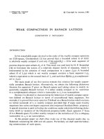
Note that we can think of the sequence (k
i
)
i≥0
as being computed along the walk
corresponding to α, and for each s ∈ [r] the entries of the sequence x
s
are obtained by
the electronic journal of combinatorics 18 (2011), #P163 11
selecting those values (k
i
)
i≥0
where the walk takes a step in direction s, see Figure 1.
As we shall see in Lemma 14 below, for any s ∈ [r] and any j ≥ 0 the number x
s,j
equals the number of vertices in the smallest component (=tree) containing a path
on j vertices in color s if Painter plays according to the strategy corresponding to
the sequence α.
The following lemma is an immediate consequence of the definitions in (3).
Lemma 11 (Monotonicity along the recursion). For any α = (α
i
)
i≥1
, α
i
∈ [r], the
sequence (k
i
)

i≥0
and in particular each of the sequences x
1
, . . . , x
r
defined in (3) is
strictly increasing.
In the following we are only interested in evaluating the above recursion for a
finite number of steps. More specifically, for integers 
1
, . . . , 
r
≥ 1 we denote by
W (
1
, . . . , 
r
) the set of finite sequences of length
d = d(
1
, . . . , 
r
) :=

s∈[r]
(
s
− 1) (4a)
with the property that for each s ∈ [r], exactly 
s

− 1 entries are equal to s. Thus
the walk corresponding to such a sequence ends at (
1
, . . . , 
r
), see Figure 1. For any
such α ∈ W (
1
, . . . , 
r
), we may evaluate the recursion (3) for the first d + 1 steps
(i.e., for i = 0, . . . , d), and define
k(α) := k
d
. (4b)
(In the last step i = d, (3d) should be ignored.)
The following proposition is the main result of this section and characterizes the
parameter k
∗
(P

1
, . . . , P

r
) from the (P

1
, . . . , P


r
)-avoidance game in terms of the
recursion defined above.
Proposition 12 (General recursion). For any integers 
1
, . . . , 
r
≥ 1, we have
k
∗
(P

1
, . . . , P

r
) = max
α∈W (
1
, ,
r
)
k(α) , (5)
where k(α) is defined in (3) and (4).
3.2 Proof of Proposit io n 12
We begin by proving that the right hand side of (5) bounds k
∗
(P

1

, . . . , P

r
) from
above. We do so by describing a Builder strategy that closely resembles the structure
of the recursion (3).
the electronic journal of combinatorics 18 (2011), #P163 12
Color 1
Color 2
1
1
2
2
3
3 4 5 6
ν
0
ν
1
ν
2
ν
3
ν
4
ν
5
ν
6
ν

7
k
0
= 1 k
1
= 2
k
2
= 3
k
3
= 6
k
4
= 9 k
5
= 10 k
6
= 11
k
7
= 1 + min(0 + 11, 1 + 10, 2 + 9)
+ min(0 + 6, 3 + 3) = 18
k
d
α = (α
1
, α
2
, . . .) = (1, 1, 2, 2, 1, 1, 1, 2, . . .)

x
1
= (0, k
0
, k
1
, k
4
, k
5
, k
6
, . . . )
x
2
= (0, k
2
, k
3
, k
7
, . . . )

1

2
Figure 1: Illustration of the definitions in (3) and (4) for the case r = 2.
Proof of Proposition 12 (upper bound). We describe a winning strategy for Builder
in the (P


1
, . . . , P

r
)-avoidance game with tree size restriction
k := max
α∈W (
1
, ,
r
)
k(α) . (6)
We may and will assume w.l.o.g. that Painter plays consistently in the sense of
Section 2, implying that if Builder has enforced a copy of some tree on the board,
then he can enforce as many additional copies of this tree as he needs. Moreover,
we will ignore such repeated steps when counting the number of steps it takes until
Builder has enforced a copy of some tree on the board. Intuitively, Builder’s strategy
follows the recursion defined in (3) for a sequence α = (α
i
)
i≥1
, α
i
∈ [r], that is
extracted step by step from Painter’s coloring decisions during the game.
Specifically, Builder maintains in each color s ∈ [r] a list T
s
= (T
s,0
, . . . , T

s,ν
s
−1
),
where T
s,0
is the null graph (v(T
s,0
) = 0) and T
s,j
, 1 ≤ j ≤ ν
s
−1, is a tree containing
a monochromatic P
j
in color s for which Builder has already enforced a copy on the
board. Initially, we have T
s
= (T
s,0
) for all s ∈ [r]. In each step, Builder does the
following: Given the lists T
s
= (T
s,0
, . . . , T
s,ν
s
−1
), s ∈ [r], he adds a new vertex v to

the board and, for each color s ∈ [r], connects it to copies of two trees from the list
T
s
for which the sum v(T
s,j
1
) + v(T
s,j
2
), j
1
+ j
2
= ν
s
−1, is minimized, in such a way
the electronic journal of combinatorics 18 (2011), #P163 13
that if Painter assigns color s to v, a path on j
1
+ j
2
+ 1 = ν
s
many vertices in color s
is created (if one of the contributing graphs is the null graph, then no corresponding
edge is added). Let σ ∈ [r] denote the color Painter assigns to v, thus creating a
tree that contains a copy of P
ν
σ
in color σ. If ν

σ
< 
σ
, then Builder adds this tree
to the end of the list T
σ
, which therefore grows by one element. Otherwise the game
ends with a monochromatic P

σ
in color σ. Let d

+ 1 denote the number of steps
until the game ends. We consider these steps indexed from 0 to d

. Moreover, let
α

∈ [r]
{1, ,d

}
denote the sequence of all coloring decisions of Painter except the last
one during Builder’s strategy. (Thus Painter’s decision in step i, 0 ≤ i ≤ d

− 1, is
given by α

i+1
, in line with (3d).) As each time Painter uses some color s ∈ [r] the

length of the list T
s
grows by exactly one, the sequence α

has at most 
s
−1 entries
equal to s.
It follows easily by induction that this Builder strategy satisfies the following
property: For each 0 ≤ i ≤ d

the lists T
s
= (T
s,0
, . . . , T
s,ν
i,s
−1
), s ∈ [r], satisfy
(v(T
s,0
), . . . , v(T
s,ν
i,s
−1
)) = (x
s,0
, . . . , x
s,ν

i,s
−1
) ,
and the tree constructed in step i has k
i
many vertices, where ν
i,s
, k
i
and the se-
quences x
1
, . . . , x
s
are defined in (3) for the given α

.
From this property it follows with Lemma 11 that the largest tree Builder con-
structs is the one in the last step of the game, and that it has k
d

many vertices.
Letting α denote any sequence from the set W(
1
, . . . , 
r
) with prefix α

, and k
d

(with
d as in (4a)) the value defined in (3) for this α, we obtain with Lemma 11 that
k
d

≤ k
d
(4b)
= k(α)
(6)
≤k ,
showing that Builder adhered to the given tree size restriction.
For proving the lower bound in Proposition 12 we will need the following obser-
vation. If the reader is deterred by the technical-looking statement, we recommend
looking at the very elementary proof first.
Lemma 13 (Choosing a color). Let 
1
, . . . , 
r
≥ 1 be integers and α ∈ W (
1
, . . . , 
r
).
Then for any integers λ
1
, . . . , λ
r
with 1 ≤ λ
s

≤ 
s
, s ∈ [r ], and λ
s
< 
s
for at least
one s ∈ [r], the following holds: There is a unique integer 0 ≤ i ≤ d − 1 such that
for σ := α
i+1
we have
ν
i,σ
= λ
σ
, (7a)
ν
i,s
≤ λ
s
, s ∈ [r] \ {σ} , (7b)
where ν
i,s
, s ∈ [r], is defined in (3a) for the given α and d = d(
1
, . . . , 
r
) is defined
in (4a). Moreover, we then have λ
σ

< 
σ
.
the electronic journal of combinatorics 18 (2011), #P163 14
Proof. Geometrically, the box B := [1, λ
1
]×···×[1, λ
r
] is contained in the larger box
[1, 
1
] ×···×[1, 
r
]. As the walk corresponding to the sequence α starts at (1, . . . , 1)
and ends at (
1
, . . . , 
r
), there is a unique first step where it leaves the box B. It is
easy to see that the starting point ν
i
of this step (which lies on the boundary of B)
is the unique integer i that satisfies the conditions of the lemma.
Consider now the following Painter strategy for the (P

1
, . . . , P

r
)-avoidance game,

which is defined for an arbitrary fixed α ∈ W (
1
, . . . , 
r
), and which we denote by
AvoidPaths
α
(P

1
, . . . , P

r
). For each new vertex v, Painter determines for each color
s ∈ [r] the number of vertices λ

s
of the longest monochromatic path in color s that
would be completed if that color were assigned to v, and defines λ
s
:= min(λ

s
, 
s
).
If (λ
1
, . . . , λ
r

) = (
1
, . . . , 
r
), then she assigns an arbitrary color to v, and the game
ends. Otherwise one of the values λ
s
is strictly smaller than 
s
. Painter then chooses
an 0 ≤ i ≤ d − 1 such that for σ := α
i+1
the relations (7) hold (such a choice is
possible by Lemma 13), and assigns color σ to v. As we have λ
σ
< 
σ
in this case,
this does not create a monochromatic P

σ
in color σ, and the game does not end in
this step.
For the rest of this paper we usually refer to a sequence α ∈ W (
1
, . . . , 
r
) as
a strategy sequence, having the above interpretation in mind. Note that the greedy
strategy analyzed in Lemma 8 is exactly AvoidPaths

α
(P

1
, . . . , P

r
) for the strategy
sequence α = (r)

r
−1
◦ (r − 1)

r−1
−1
◦ ··· ◦ (1)

1
−1
. Here and throughout we use ◦ to
denote concatenation of sequences, and integer exponents to indicate repetitions.
The next lemma states the strategy invariant that we already briefly mentioned
when we introduced the recursion (3).
Lemma 14 (AvoidPaths() strategy invariant). Playing according to the strategy
AvoidPaths
α
(P

1

, . . . , P

r
) ensures that the following invariant holds throughout,
except possibly in the last step when the game ends: For each s ∈ [r] and each
0 ≤ t ≤ 
s
− 1, each monochromatic P
t
in color s on the board is contained in a
component (=tree) with at least x
s,t
vertices, where x
s,t
is defined in (3) for the given
α.
As we shall see, the above invariant is also maintained in the last step when the
game ends, but for technical reasons we do not prove this here.
Proof. To show that this invariant holds, we argue by induction over the number of
steps of the game: Initially, no graph is present on the board, and the statement is
trivially true (with t = 0 and x
s,0
= 0). For the induction step consider a fixed step
where the game does not end, and let λ
s
, s ∈ [r], be as defined in Painter’s strategy.
Furthermore, let i denote the index guaranteed by Lemma 13 for these values λ
s
,
the electronic journal of combinatorics 18 (2011), #P163 15

and let σ = α
i+1
denote the color Painter assigns to the new vertex v in this step.
Clearly, the invariant is maintained for all colors s ∈ [r]\{σ}, and it remains to show
that it holds for σ. By Lemma 11 we have
x
σ,0
< x
σ,1
< ··· < x
σ,
σ
−1
,
implying that it suffices to consider a longest monochromatic path in color σ that is
completed by Painter’s decision to assign color σ to v. Let Q
σ
denote such a path,
and set t := v(Q
σ
). As the game does not end in the current step, we have t ≤ 
σ
−1.
By definition of Painter’s strategy, we have
λ
σ
= t , (8)
and for each s ∈ [r] \ {σ}, assigning color s to v would have completed some (not
necessarily maximal) path Q
s

in color s on λ
s
vertices. Note that the paths Q
1
, . . . , Q
r
only share the vertex v, and that v divides each of these paths into two paths Q
s,1
and Q
s,2
which for j
s,1
:= v(Q
s,1
) and j
s,2
:= v(Q
s,2
) satisfy
j
s,1
+ j
s,2
= λ
s
− 1
(7)
≥ν
i,s
− 1 . (9)

Furthermore, observe that the 2r paths Q
s,1
and Q
s,2
, s ∈ [r], were contained in 2r
distinct components (=trees) T
s,1
and T
s,2
before being joined by the vertex v in the
current step. (If Q
s,1
or Q
s,2
has no vertices, then we also let T
s,1
or T
s,2
be the null
graph, i.e., the graph with empty vertex set.) By induction we have
v(T
s,1
) ≥ x
s,j
s,1
,
v(T
s,2
) ≥ x
s,j

s,2
.
(10)
Combining our previous observations, we obtain that the vertex v is contained in a
tree T satisfying
v(T ) = 1 +

s∈[r]

v(T
s,1
) + v(T
s,2
)

(10)
≥ 1 +

s∈[r]
(x
s,j
s,1
+ x
s,j
s,2
)
(3c),(9)
≥ k
i
, (11)

where we also used Lemma 11 in the last step. Combining (3d), (7a) and (8) shows
that the right hand side of (11) equals x
σ,t
, proving that the claimed invariant holds.
We are now in a position to prove the lower bound in Proposition 12. The
argument is very similar to the inductive argument in the previous proof, but due to
some subtleties we have to treat the step in which the game ends separately.
the electronic journal of combinatorics 18 (2011), #P163 16
Proof of Proposition 12 (lower bound). We will argue that the strategy Avoid-
Paths
α
(P

1
, . . . , P

r
) is a winning strategy for Painter in the (P

1
, . . . , P

r
)-avoidance
game with tree size restriction k(α ) − 1, where k(α) is defined in (3) and (4). Op-
timizing over the choice of α ∈ W (
1
, . . . , 
r
), we thus obtain a winning strategy for

Painter in the game with tree size restriction max
α∈W (
1
, ,
r
)
k(α) − 1, as required.
Let α ∈ W (
1
, . . . , 
r
) be fixed and suppose Painter plays according to the strategy
AvoidPaths
α
(P

1
, . . . , P

r
). Suppose for the sake of contradiction that Painter loses
with a monochromatic path P

s
in some color s ∈ [r]. By the definition of Painter’s
strategy, this means that in the last step of the game assigning any of the colors
s ∈ [r ] to the last vertex v would complete a path P

s
in color s. This implies that

in each color s ∈ [r] the vertex v joins two (not necessarily maximal) paths Q
s,1
and
Q
s,2
in color s which for j
s,1
:= v(Q
s,1
) and j
s,2
:= v(Q
s,2
) satisfy
j
s,1
+ j
s,2
= 
s
− 1 . (12)
Denoting for every s ∈ [r] by T
s,1
and T
s,2
the components (=trees) that were joined
by v and that contain Q
s,1
and Q
s,2

, respectively, we obtain from Lemma 14 that the
vertex v is contained in a tree T satisfying
v(T ) = 1 +

s∈[r]

v(T
s,1
) + v(T
s,2
)

≥ 1 +

s∈[r]
(x
s,j
s,1
+ x
s,j
s,2
)
(3c),(4b),(12)
≥ k(α) ,
where in the last step we also used that for d defined in (4a) we have ν
d
= (
1
, . . . , 
r

).
This yields the desired contradiction and completes the proof.
3.3 Exact values of k
∗
(P

, 2) for small values of 
The values in Table 1 were found by implementing the recursion in (3) and (4) and
using Proposition 12. The computationally most expensive part in this approach is
the maximization in (5), as e.g. for the (symmetric) P

-avoidance game with r = 2
colors it requires maximizing over all strategy sequences from W (, ), of which there
are

2(−1)
−1

= 4
(1+o(1))
many. However, by using an appropriate branch-and-bound
technique, the set of strategy sequences to be considered in the maximization can be
reduced substantially. A program that implements this and further optimizations to
compute k
∗
(P

, 2) is available from the authors’ websites [1].
We conclude this section by giving an example of a Painter strategy for the
P


-avoidance game with r = 2 colors that outperforms the greedy strategy. For
 = 28, there are four strategy sequences from the set W (28, 28) achieving the
optimal performance k
∗
(P
28
, 2) = 28
2
+ 7 = 791 (cf. Table 1). They are given
the electronic journal of combinatorics 18 (2011), #P163 17
by α = (1)
6
◦ (2, 2) ◦ (1)
7
◦ (2) ◦ (1)
14
◦ (2)
24
, α

= (1, 1, 2, 1, 2, 2) ◦(1)
24
◦ (2)
24
, and
the sequences α and α

that are obtained from α and α


by interchanging the 1 and
2 entries, exploiting the obvious symmetry.
4 Analyzing the recursion
In this section we prove Theorems 4–7 by analyzing the recursion defined in (3) and
(4) and using Proposition 12. We focus on the asymmetric path-avoidance game in
most of the upcoming arguments, and derive our results for the symmetric game at
the very end. For the rest of this paper we restrict our attention to the case of r = 2
colors.
4.1 Asymptotic behavio ur
A crucial ingredient in our analysis of the recursion in (3) and (4) is the study of
its asymptotic behaviour along a walk as described in Section 3.1 which after some
initial turns moves towards infinity only along one coordinate direction (think e.g.
of infinitely extending the walk in Figure 1 in coordinate direction 1). The following
completely self-contained lemma is the basis for this approach.
For any sequence (x
ν
)
ν≥0
we define the corresponding sequence of first differences
as ∆(x) := (x
ν+1
− x
ν
)
ν≥0
.
Lemma 15 (Recursion becomes periodic). Let x
0
, . . . , x
t

and β be arbitrary integers,
and recursively define
x
ν
:= β + min
j
1
,j
2
≥0:
j
1
+j
2
=ν−1
(x
j
1
+ x
j
2
) , ν ≥ t + 1 . (13)
Furthermore, let p be an integer from the set arg min
0≤j≤t
x
j
+β
j+1
. Then the sequence
∆(x) = (x

ν+1
−x
ν
)
ν≥0
becomes periodic with period length p+ 1, and for all ν ≥ t+ 1
we have
x
ν
− x
ν−(p+1)
≤ x
p
+ β (14)
with equality for all large enough ν. Moreover, for all k ≥ 1 we have
x
p+k(p+1)
− x
p
≥ k(x
p
+ β) . (15)
Note that Lemma 15 quantifies the asymptotic behaviour of the recursion (13):
In the long run, the values will change by x
p
+ β every p + 1 steps, i.e., for ν → ∞
we have
x
ν
= (δ + o(1)) ·ν ,

the electronic journal of combinatorics 18 (2011), #P163 18
where
δ = δ(x
0
, . . . , x
t
, β) := min
0≤j≤t
x
j
+ β
j + 1
. (16)
Proof. For any two integers a ≥ 1 and b, applying the transformation
y
ν
= a(x
ν
+ β) − b(ν + 1) (17)
to (13) yields an integer sequence (y
ν
)
ν≥0
that satisfies the recursion
y
ν
= min
j
1
,j

2
≥0:
j
1
+j
2
=ν−1
(y
j
1
+ y
j
2
) , ν ≥ t + 1 . (18)
Furthermore, by (17) the first differences of the sequences (x
ν
)
ν≥0
and (y
ν
)
ν≥0
are
related via
∆(y) = a∆(x) −b . (19)
Applying the transformation (17) with
a := p + 1 and b := x
p
+ β , (20)
we obtain with the definition of p in the lemma that y

p
= 0 and y
ν
≥ 0 for all
0 ≤ ν ≤ t. By these initial conditions and by (18), all elements of the sequence
(y
ν
)
ν≥0
are non-negative. Furthermore, using that y
p
= 0 it follows from (18) that
y
ν
≤ y
ν−(p+1)
for all ν ≥ t + 1 . (21)
Combining this with the non-negativity of the sequence (y
ν
)
ν≥0
, we obtain that for
each residue class modulo p + 1 the corresponding subsequence of (y
ν
)
ν≥0
becomes
constant, and that consequently the sequence itself becomes periodic with period
length p + 1. It follows that the sequence ∆(y) and by (19) also the sequence ∆(x)
become periodic with period length p + 1.

Note that for all ν ≥ t + 1 we have
x
ν
− x
ν−(p+1)
(19)
=
y
ν
− y
ν−(p+1)
+ b(p + 1)
a
(21)
≤
b(p + 1)
a
(20)
= x
p
+ β ,
with equality for all large enough ν, proving (14).
Similarly, using the non-negativity of the sequence (y
ν
)
ν≥0
and y
p
= 0 we obtain
for all k ≥ 1

x
p+k(p+1)
− x
p
(19)
=
y
p+k(p+1)
− y
p
+ bk(p + 1)
a
≥
bk(p + 1)
a
(20)
= k(x
p
+ β) ,
proving (15).
the electronic journal of combinatorics 18 (2011), #P163 19
4.2 Explicit version of Theorem 5
Using Lemma 15 we will show that asymptotically optimal Painter strategies for the
asymmetric (P

, P
c
)-avoidance game (i.e., strategies achieving the lower bound stated
in Theorem 5) can be constructed as follows. Intuitively, we distinguish two phases of
the corresponding walks: a short initial ‘preparation’ phase and a long ‘payoff’ phase,

which is just a straight segment of the walk extending into coordinate direction 1.
The goal of the preparation phase is not to directly optimize the resulting recursion
values during this phase, but to optimize the constant δ as defined in (16) that arises
when applying Lemma 15 to the payoff phase.
These ideas lead to the following definition of the constant δ(c) appearing in
Theorem 5. For any strategy sequence α ∈ W (, c) we define
β(α) := 1 + min
j
1
,j
2
≥0:
j
1
+j
2
=c−1
(x
2,j
1
+ x
2,j
2
) , (22a)
δ(α) := min
0≤j≤−1
x
1,j
+ β(α)
j + 1

, (22b)
where x
1
= (x
1,0
, . . . , x
1,−1
) and x
2
= (x
2,0
, . . . , x
2,c−1
) are defined via the recursion
(3). Using those definitions we set
δ(1) := 1 , (22c)
and for any c ≥ 2,
δ(c) := sup
≥1
α∈W (,c): α
+c−2
=2
δ(α) , (22d)
where the condition α
+c−2
= 2 expresses that the last step of the walk corresponding
to α is towards the second coordinate. We will see in Lemma 17 below that δ(c) is
indeed a well-defined finite value.
Theorem 16 (Explicit version of Theorem 5). For any c ≥ 1 and any  ≥ 1 we have
k

∗
(P

, P
c
) ≤ δ(c) ·
and
k
∗
(P

, P
c
) ≥ (δ(c) − o(1)) ·  ,
where δ(c) is defined in (22), and o(1) stands for a non-negative function of c and 
that tends to 0 for c fixed and  → ∞.
We prove Theorem 16 (and thus Theorem 5) in the next section.
the electronic journal of combinatorics 18 (2011), #P163 20
4.3 Proof of Theorem 16
We will prove the following three lemmas by induction. Note that Lemma 19 is
exactly the upper bound part of Theorem 16, and that moreover Lemma 17 yields
the upper bound part of Theorem 7 (we have log
2
(3) = 1.584 . . . < 1.59).
Lemma 17 (Upper bound for δ(c)). For any c ≥ 1 we have δ(c) ≤ c
log
2
(3)
.
Lemma 18 (Monotonicity of δ(c)). For all 1 ≤ c ≤ c we have δ(c ) ≤ δ(c).

Lemma 19 (Upper bound for k
∗
(P

, P
c
) via δ(c)). For any c ≥ 1 and any  ≥ 1 we
have k
∗
(P

, P
c
) ≤ δ(c) ·.
Proof of Lemma 17, 18 and 19. We argue by induction on c. For c = 1 all claims
are trivially satisfied. For the induction step let c ≥ 2.
Induction step for Lemma 17. For any fixed  ≥ 1 consider an arbitrary fixed
strategy sequence α ∈ W (, c) with α
+c−2
= 2. Note that α can be uniquely written
in the form
α = (1)

1
−1
◦ (2) ◦ (1)

2
−
1

◦ (2) ◦ ··· ◦ (1)

c−1
−
c−2
◦ (2) , (23)
where 1 ≤ 
1
≤ 
2
≤ ··· ≤ 
c−2
≤ 
c−1
= .
In the following we derive upper bounds for the entries of the sequences x
1
and x
2
defined in (3) for this α. For any 1 ≤ j ≤ c −1 we define α
(j)
as the maximal prefix
of α containing exactly j − 1 entries equal to 2. By (23) we have α
(j)
∈ W(
j
, j).
Moreover, by the definitions in (3) and (4) and by Proposition 12 we have
x
2,j

= k
(
j
−1)+(j−1)
= k(α
(j)
)
(5)
≤k
∗
(P

j
, P
j
) , 1 ≤ j ≤ c −1 . (24)
By induction and Lemma 19 we hence obtain from (24) that
x
2,j
≤ δ(j) · 
j
, 1 ≤ j ≤ c −1 . (25)
Using that by (3) and (23) the integers x
1,
j
−1
and x
2,j
correspond to sequence
elements k

i
and k
i

as defined in (3c) with i < i

, we obtain with Lemma 11 that
x
1,
j
−1
≤ x
2,j
− 1
(25)
≤ δ(j) ·
j
− 1 , 1 ≤ j ≤ c − 1 . (26)
By setting j
1
= (c − 1)/2 and j
2
= (c − 1)/2 in (22a) we obtain
β(α)
(22a)
≤ 1+x
2,(c−1)/2
+x
2,(c−1)/2
≤ 1+2x

2,(c−1)/2
(25)
≤ 1+2δ(

c−1
2

)·
(c−1)/2
, (27)
the electronic journal of combinatorics 18 (2011), #P163 21
where we again used Lemma 11 in the second estimate. Similarly, setting j =

(c−1)/2
− 1 in (22b) yields
δ(α)
(22b)
≤
x
1,
(c−1)/2
−1
+ β(α)

(c−1)/2
(26),(27)
≤ 3 · δ(

c−1
2


) . (28)
As the bound in (28) holds for all  ≥ 1 and all strategy sequences α ∈ W (, c) with
α
+c−2
= 2 simultaneously, we obtain with the definition in (22d) that
δ(c) ≤ 3 · δ(
c−1
2
) ≤ 3 ·
c−1
2

log
2
(3)
≤ 3 ·

c
2

log
2
(3)
= c
log
2
(3)
,
where the second estimate is the induction hypothesis. This completes the proof of

Lemma 17.
Induction step for Lemma 18. By induction we have δ(1) ≤ ··· ≤ δ(c − 1), so
it suffices to show that δ(c − 1) ≤ δ(c). Note that δ(c) is a well-defined finite value
by Lemma 17. For c = 2, observe that the strategy sequence α = (2) ∈ W (1, 2)
yields β(α) = 2 and δ(α) = 2 and consequently guarantees a lower bound of δ(2) ≥
2, implying in particular that δ(1) ≤ δ(2) (recall (22c)). For c ≥ 3 we argue as
follows: For each strategy sequence α
−
∈ W(, c − 1) with α
−
+(c−1)−2
= 2 consider
the extended sequence α := α
−
◦ (2) ∈ W (, c). By Lemma 11 and (22a) we have
β(α
−
) < β(α), which by (22b) implies that δ(α
−
) < δ(α). Using (22d) this shows
that δ(c − 1) ≤ δ(c), completing the proof of Lemma 18.
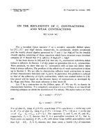
Induction step for Lemma 19. For the reader’s convenience, Figure 2 illustrates
the notations used in this proof.
Let  ≥ 1 and α ∈ W (, c) be fixed. We show that for k(α) as defined in (3)
and (4) we have k(α) ≤ δ(c) · , from which the claim follows by Proposition 12.
For the proof it is convenient to extend the sequences x
1
= (x
1,0
, . . . , x

1,−1
) and
x
2
= (x
2,0
, . . . , x
2,c−1
) defined in (3) for the given α by setting
x
1,
:= k
d
(4b)
= k(α) (29)
with d = d(, c) defined in (4a). Let 

be such that α = α

◦(1)
−

with α

∈ W(

, c)
and α




+c−2
= 2. Fixing some integer
p ∈ arg min
0≤j≤

−1
x
1,j
+ β(α

)
j + 1
, (30)
where β(α

) is defined in (22a), we have
x
1,p
+ β(α

)
p + 1
(22b),(30)
= δ(α

)
(22d)
≤ δ(c) . (31)
the electronic journal of combinatorics 18 (2011), #P163 22

Color 1
Color 2
1
1
 =

 + m(p + 1)




c
c
p
p + 1p + 1
α ∈ W (, c)α

∈ W(

, c)
α ∈ W (

, c )
Figure 2: Notations used in the proof of Lemma 19.
Let

 ≤ 

− 1 be the largest integer such that
 =


 + m(p + 1) (32)
for some integer m.
By (3), (29) and the definition of β(α

) in (22a) we have
x
1,ν
= β(α

) + min
j
1
,j
2
≥0:
j
1
+j
2
=ν−1
(x
1,j
1
+ x
1,j
2
) , 

≤ ν ≤  .

We may hence apply Lemma 15, and using (30) we obtain that
x
1,
(32)
= x
1,
b
+m(p+1)
(14)
≤ x
1,
b

+ m(x
1,p
+ β(α

)) . (33)
If

 ≥ 1, we let c denote the maximal value of ¯c for which W (

, ¯c) contains a
prefix of α

, and we let α ∈ W (

, c ) denote the corresponding prefix (see Figure 2).
Clearly we have c < c and
k(α)

(3),(4)
= x
1,
b

. (34)
As c < c we may apply the induction hypothesis and obtain together with Proposi-
tion 12 that
k(α)
(5)
≤k
∗
(P
b

, P
bc
) ≤ δ(c ) ·

 ,
which combined with (34) and Lemma 18 yields
x
1,
b

≤ δ(c) ·

 . (35)
the electronic journal of combinatorics 18 (2011), #P163 23
If


 = 0, then both sides of this inequality vanish, and (35) holds trivially.
Combining our previous observations we obtain
k(α)
(29),(33)
≤ x
1,
b

+ m(x
1,p
+ β(α

))
(31),(35)
≤ δ(c) · (

 + m(p + 1))
(32)
= δ(c) ·  ,
completing the proof of Lemma 19.
It remains to prove the lower bound in Theorem 16.
Proof of Theorem 16 (lower bound). As in the proof of Lemma 19 it is also conve-
nient here to extend the definition in (3d) for any α ∈ W (, c) by setting
x
1,
:= k
d
(4b)
= k(α) (36)

with d = d(, c) defined in (4a). Note that the claim holds trivially if c = 1, so we
consider a fixed c ≥ 2 in the following. By the definition in (22d) there are families
(
t
)
t≥0
and (α
(t)
)
t≥0
, where α
(t)
∈ W(
t
, c) with α
(t)

t
+c−2
= 2, satisfying
lim
t→∞
δ(α
(t)
) = δ(c) . (37)
Fix any such strategy sequence α
(t)
, and for every  ≥ 
t
consider the extended

sequence α
(t)
:= α
(t)
◦ (1)
−
t
∈ W (, c). Using (22a) we obtain that for any such
extended sequence α
(t)
, the sequence x
1
= (x
1,0
, . . . , x
1,
) defined in (3) and (36)
satisfies
x
1,ν
= β(α
(t)
) + min
j
1
,j
2
≥0:
j
1

+j
2
=ν−1
(x
1,j
1
+ x
1,j
2
) , 
t
≤ ν ≤  .
Moreover, by (36) we have k(α
(t)
) = x
1,
. By the first part of Lemma 15 and the
definition in (22b) we thus have
k(α
(t)
) = (δ(α
(t)
) + o(1)) ·
for c and t fixed and  → ∞. Here we used that for all large enough indices, (14)
holds with equality. Combining this with (37) and applying Proposition 12 yields
that
k
∗
(P
c

, P

) ≥ (δ(c) + o(1)) · 
for c fixed and  → ∞. Moreover, the upper bound given by Lemma 19 shows that
the term o(1) must be non-positive.
the electronic journal of combinatorics 18 (2011), #P163 24
4.4 Proof of Theorem 6
In this section we derive the exact values of δ(c) stated in Theorem 6 by carrying out
explicitly the optimization over lattice walks that appears in the definition (22d).
Note that for small values of c, the walk corresponding to a strategy sequence α ∈
W (, c) has only few turning points. We will derive upper bounds for the entries of the
sequences x
1
and x
2
computed by the recursion (3) as a function of the 1-coordinates
of these turning points. To do so we will only consider a few carefully selected terms
when evaluating the minimization in (3c). The upper bound on δ(c) we obtain this
way is the minimum over a small number of functions of 1-coordinates of turning
points, and turns out to be irrational. We will derive asymptotically matching lower
bounds by describing families of strategy sequences for which the ratios between
the 1-coordinates of successive turning points approximate the optimal (irrational!)
ratios.
We only give the proof for c = 4 here. The similar but more complicated proofs
for c ∈ {5, 6} can be found in [10].
Proof of δ(4) =
1
2
(
√

13 + 5). Consider a strategy sequence α ∈ W(, 4) that satisfies
α
+4−2
= 2, and note that α can be uniquely written in the form
α = (1)

1
−1
◦ (2) ◦ (1)

2
−
1
◦ (2) ◦ (1)
−
2
◦ (2) ,
where 1 ≤ 
1
≤ 
2
≤ .
Let p ≥ 1 and 0 ≤ m < 
1
be the unique integers satisfying

2
= p
1
+ m . (38)

The recursion (3) yields by straightforward calculations that
x
1,j
= j , 0 ≤ j ≤ 
1
− 1 , (*)
x
2,1
= 
1
,
x
1,2
1
−1
≤ x
1,
1
−1
+ x
1,
1
−1
+ x
2,1
+ 1 = 3
1
− 1 ,
x
1,3

1
−1
≤ x
1,2
1
−1
+ x
1,
1
−1
+ x
2,1
+ 1 ≤ 5
1
− 1 ,
. . .
x
1,p
1
−1
≤ x
1,(p−1)
1
−1
+ x
1,
1
−1
+ x
2,1

+ 1 ≤ 2p
1
− 
1
− 1 , (**)
x
1,
2
−1
≤ x
1,p
1
−1
+ x
1,m−1
+ x
2,1
+ 1 ≤ 2p
1
+ m − 1
(38)
= 2
2
− m − 1 , (***)
x
2,2
≤ x
1,p
1
−1

+ x
1,m
+ x
2,1
+ 1 ≤ 2p
1
+ m
(38)
= 2
2
− m ,
(39)
the electronic journal of combinatorics 18 (2011), #P163 25