ENERGY MANAGEMENT HANDBOOKS phần 6 pdf

INDUSTRIAL INSULATION 451
Table 1 5.2 Equivalent thickness values for even insulation thicknesses.
Actual Thickness (in.)
Nominal Pipe
Size (in.) r
1
1 1-1/2 2 2-1/2 3 3-1/2 4
1/2 0.420 1.730 2.918 4.238 5.662 7.172 8.755 10.402
3/4 0.525 1.626 2.734 3.966 5.297 6.712 8.199 9.747
1 0.658 1.532 2.563 3.711 4.953 6.275 7.665 9.117
1-1/4 0.830 1.447 2.405 3.472 4.626 5.856 7.153 8.507
1-1/2 0.950 1.403 2.321 3.342 4.449 5.629 6.872 8.171
2 1.188 1.337 2.195 3.148 4.177 5.276 6.436 7.648
2-1/2 1.438 1.287 2.099 2.997 3.968 5.001 6.093 7.234
3 1.750 1.242 2.012 2.858 3.771 4.742 5.768 6.840
3-1/2 2.000 1.217 1.959 2.772 3.649 4.582 5.564 6.592
4 2.250 1.194 1.916 2.704 3.549 4.448 5.396 6.386
4-1/2 2.500 1.178 1.880 2.645 3.464 4.337 5.253 6.211
5 2.781 1.163 1.846 2.590 3.388 4.231 5.118 6.043
6 3.313 1.138 1.799 2.510 3.270 4.071 4.911 5.790
7 3.813 1.120 1.761 2.453 3.184 3.956 4.759 5.604
8 4.313 1.108 1.737 2.407 3.116 3.863 4.644 5.452
9 4.813 1.097 1.714 2.369 3.056 3.783 4.541 5.330
10 5.375 1.088 1.693 2.333 3.007 3.714 4.450 5.214
11 5.875 1.079 1.675 2.305 2.972 3.663 4.383 5.123
12 6.375 1.076 1.662 2.286 2.936 3.619 4.321 5.048
14 7.000 1.069 1.647 2.265 2.900 3.569 4.258 4.969
16 8.000 1.059 1.639 2.231 2.858 3.504 4.178 4.866
18 9.000 1.053 1.622 2.206 2.822 3.449 4.110 4.776
20 1 0.000 1.048 1.608 2.188 2.789 3.411 4.051 4.711
24 12.000 1.040 1.589 2.163 2.736 3.347 3.971 4.598

30 15.000 1.032 1.572 2.122 2.704 3.281 3.874 4.497
Source: Ref. 1 6.
surface temperature is directly related to
the surface resistance R
s
, which in turn
depends on the emittance of the surface.
As a result, an aluminum jacket will be
hotter than a dull mastic coating over
the same amount of insulation. This is
demonstrated below.
Calculation
The objective is to calculate the amount of
insulation required to attain a specifi c sur-
face temperature. As noted earlier,
t
h
– t
s
R
1
=
t
s
– t
a
R
s

Therefore,

R
1
= R
s
t
h
– t
s
t
s
– t
a
=
tk
k
flat =
Eq tk
k
pipe
Therefore,
tk or Eq tk = kR
s
t
h
– t
s
t
s

– t
a

Fig. 15.3 Equivalent thickness chart. (From Ref. 16.)
452 ENERGY MANAGEMENT HANDBOOK
Table 15.3 Equivalent thickness values for simplifi ed insulation thicknesses.
Actual Thickness (in.)
Nominal Pipe
Size (in.) r1 1 1-1/2 2 2-1/2 3 3-1/2 4
1/2 0.420 1.730 3.053 4.406 6.787 8.253 9.972 12.712
3/4 0.523 1.435 2.660 3.885 5.996 7.447 8.965 10.642
1 0.638 1.715 2.770 4.013 5.358 6.702 8.112 9.581
1-1/4 0.830 1.281 2.727 3.333 4.552 5.777 7.070 8.420
1-1/2 0.950 1.457 2.382 4.025 5.253 6.476 7.759 9.179
2 1.188 1.438 2.367 3.398 4.446 5.561 6.733 8.027
2-1/2 1.438 1.383 2.765 3.657 4.737 5.815 7.015 8.195
3 1.750 1.286 2.114 2.968 3.889 4.868 5.965 7.046
3-1/2 2.000 1.625 2.459 3.258 4.166 5.251 6.266 7.256
4 2.230 1.281 2.010 2.806 3.659 4.059 5.577 6 543
4-1/2 2.300 1.564 2.351 3.152 4.905 4.962 5.907 7 080
5 2.781 1.202 1.893 2.639 3.489 4.339 5.230 6.461
6 3.313 1.138 1.799 2.555 3.317 4.122 5.237 6.015
7 3.813 1.804 2.495 3.230 4.153 4.969 5.821
8 4.313 1.776 2.445 3.391 4.010 4.842 5.768
9 4.813 1.752 2.579 3.232 3.971 4.786 5.583
10 5.375 1.810 2.457 3.108 3.850 4.591 5.361
11 5.875 1.793 2.428 3.140 3.793 4.519 5.271
12 6.375 1.777 2.405 3.103 3.745 4.456 5.241
14 7.000 1.647 2.265 2.900 3.569 4.258 4.969
16 8.000 1.639 2.231 2.858 3.504 4.178 4.866

18 9.000 1.622 2.206 2.822 3.449 4.110 4.776
20 10.000 1.608 2.188 2.789 3.411 4.051 4.711
24 12.000 1.589 2.163 2.736 3.347 3.971 4.598
30 15.000 1.572 2.122 2.704 3.281 3.874 4.497
Source: Ref. 16.
Table 15.4 R
s
Values
a
(hr • ft
2
°F/Btu).
Still Air
Plain, Fabric,
t
s
– t
a
Dull Metal: Aluminum: Stainless Steel:
(°F) ε = 0.95 ε = 0.2 ε = 0.4

10 0.53 0.90 0.81
25 0.52 0.88 0.79
50 0.50 0.86 0.76
75 0.48 0.84 0 75
100 0.46 0.80 0 72
With Wind Velocities
Wind Velocity
(mph)

5 0.35 0.41 0.40
10 0.30 0.35 0.34
20 0.24 0.28 0.27
Source: Courtesy of Johns-Manville, Ref. 16.
a
For heat-loss calculations, the effect of R
s
is small compared to R
I
, so the accuracy of R
s
is not critical. For surface temperature calculations, Rs is
the controlling factor and is therefore quite critical. The values presented in Table 15.4 are commonly used values for piping and fl at surfaces. More
precise values based on surface emittance and wind velocity can be found in the references.
INDUSTRIAL INSULATION 453
Example. For a 4-in. pipe operating at 700°F in an 85°F
ambient temperature with aluminum jacketing over the
insulation, determine the thickness of calcium silicate
that will keep the surface temperature below 140°F.
Since this is a pipe, the equivalent thickness must fi rst
be calculated and then converted to actual thickness.
STEP 1. Determine k at t
m
= (700 + 140)/2 = 420°F. k =
0.49 from Table 15.1 or appendix Figure 15.A1 for calcium
silicate.
STEP 2. Determine R
s
from Table 15.4 for aluminum.
t

s
– t
a
= 140 – 85 = 55. So R
s
= 0.85.
STEP 3. Calculate Eq tk:
700 – 140
Eq tk = (0.49)(0.85) —————
140 – 85
= 4.24 in.
STEP 4. Determine the actual thickness from Table 15.2.
The effect of 4.24 in. on a 4-in. pipe can be accomplished
by using 3 in. of insulation.
Note: Thickness recommendations are always
increased to the next 1-in. increment. If a surface tem-
perature calculation happens to fall precisely on an even
increment (such as 3 in.), it is advisable to be conserva-
tive and increase to the next increment (such as 3-1/2
in.). This reduces the criticality of the R
s number used.
In the preceding example, it would not be unreasonable
to recommend 3-1/2 in. of insulation, since it was found
to be so close to 3 in.
To illustrate the effect of surface type, consider he
same example with a mastic coating.
Example. From Table 15.4, R
s
= 0.50, so
700 – 140

Eq tk = (0.49)(0.50) —————
140 – 85
= 2.49 in.
This corresponds to an actual thickness require-
ment on a 4-in. pipe of 2 in. This compares with 3 in.
required for an aluminum-jacketed system. It is of inter-
est to note that even though the aluminum system has
a higher surface temperature, the actual heat loss is less
because of the higher surface resistance value.
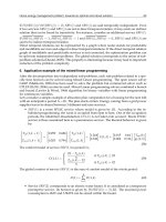
Graphical Method
The calculations illustrated above can also be car-
ried out using graphs which set the heat loss through
the insulation equal to the heat loss off the surface, fol-
lowing the discussion in Section 15.4.2.
Figure 15.4 will be used for several different cal-
culations. The following example gives the four-step
procedure for achieving the desired surface temperature
for personnel protection. The accompanying diagram
outlines this procedure.
Example. We follow the procedure of the fi rst example,
again using aluminum jacketing.
STEP 1. Determine t
s
– t
a
, 140 – 85 = 55°F.
STEP 2. In the diagram, proceed vertically from (a)
of ∆t = 55 to the curve for aluminum jacketing (b).
STEP 2a. Although not required, read the heat loss
Q = 65 Btu/hr ft

2
) (c).
STEP 3. Proceed to the right to (d), the appropriate
curve for t
h
– t
s
= 700 – 140 = 560°F. Interpolate between
lines as necessary.
STEP 4. Proceed down to read the required insulation
resistance R
t
= 8.6 at (e). Since R = tk/k or Eq tk/k,
tk or Eq tk = R
I
k
700 + 140
t
m
= ——————— = 420°F
2

k = 0.49 from appendix Figure 15.A1 and
tk or Eq tk = (8.6) (0.49) = 4.21 in.
which compares well with the 4.24 in. from the earlier
calculation.
The conversion of Eq tk to actual thickness re-
quired for pipe insulation is done in the same manner,
using Figure 15.3.
A better understanding of the procedure involved

in utilizing this quick graphical method will be obtained
454 ENERGY MANAGEMENT HANDBOOK
after working through the remainder of the calculations
in this section.
15.4.4 Condensation Control
On cold systems, either piping or equipment, in-
sulation must be employed to prevent moisture in the
warmer surrounding air from condensing on the colder
surfaces. The insulation must be of suffi cient thickness
to keep the insulation surface temperature above the
dew point of the surrounding air. Essentially, the cal-
culation procedures are identical to those for personnel
protection except that the dew-point temperature is
substituted for the desired surface temperature. (Note:
The surface temperature should be kept 1 or 2° above
the dew point to prevent condensation at that tempera-
ture.)
Dew-Point Determination
The condensation (saturation) temperature, or dew
point, is dependent on the ambient dry-bulb and wet-
bulb temperatures. With these two values and the use of
a psychrometric chart, the dew point can be determined.
However, for most applications, the relative humidity is
more readily attainable, so the dew point is determined
using dry-bulb temperature and relative humidity rather
than wet-bulb. Table 15.5 is used to fi nd the proper dew-
point temperature.
Calculation
This equation is identical to the previous surface-
temperature problem except that the surface tempera-

ture ts now takes on the value of the dew point of the
ambient air. Also, t
h
now represents the cold operating
temperature.

tk or Eq tk = kR
s
t
h
–t
s
t
s
–t
a
Fig. 15.4 Heat loss and surface temperature graphical method. (From Ref. 16.)
INDUSTRIAL INSULATION 455
Example. For a 6-in diameter chilled-water line op-
erating at 35°F in an ambient of 90°F and 85% RH,
determine the thickness of fi berglass pipe insulation
with a composite kraft paper jacket required to prevent
condensation.
STEP 1. Determine the dew point (DP) using either
a psychrometric chart or Table 15.5. DP at 90°F and 85%
RH = 85°F. (In Step 5, the thickness is rounded up, which
yields a higher temp.)
STEP 2. Determine k at t
m
= (35 + 85)/2 = 60°F. k at

60°F = 0.23, from Table 15.1 or appendix Figure 15.A2.
STEP 3. Determine R
s from Table 15.4. ∆t here is
(t
a
, – t
s
) rater than (t
s
– t
a
), t
a
– t
s
= 90 – 85 = 5°F, R
s
=
0.54.
STEP 4. Calculate Eq tk.
Eq tk = 0.23 0.54
35 – 85
85 – 90
=1.24in.
STEP 5. Determine the actual thickness from Fig-
ure 15.2 for 6-in. pipe, 1.24 in. Eq tk. The actual thickness
is 1.5 in.
Graphical Method
The graphical procedures are as described in
Section 15.4.3. As the applications become colder, it is

apparent that the required insulation thicknesses will
become larger, with R
I
values toward the right side of
Figure 15.4. It is suggested that the graphical procedure
not be used when the resulting R
I
values must be de-
termined from a very fl at portion of the (t
h
– t
s
) curve
(anytime the numbers are to the far right of Figure 15.4).
It is diffi cult to read the graph with suffi cient accuracy,
particularly in light of the simplicity of the mathematical
calculation.
Thickness Chart for Fiberglass Pipe Insulation
Table 15.6 gives the thickness requirements for fi -
berglass pipe insulation with a white, all-purpose jacket
in still air. The calculations are based on the lowest
Table 15.5 Dew-point temperature.
Dry-
Bulb Percent Relative Humidity
Temp.
(°F) 10 15 20 25 30 35 40 45 50 55 60 65 70 75 80 85 90 95 100
5 – 35 – 30 – 25 – 21 – 17 – 14 – 12 – 10 – 8 – 6 – 5 – 4 – 2 – 1 1 2 3 4 5
10 – 31 – 25 – 20 – 16 – 13 – 10 – 7 – 5 – 3 – 2 0 2 3 4 5 7 8 9 10
15 – 28 – 21 – 16 – 12 – 8 – 5 – 3 – 1 1 3 5 6 8 9 10 12 13 14 15
20 – 24 – 16 – 8 – 4 – 2 2 4 6 8 10 11 13 14 15 16 18 19 20

25 – 20 – 15 – 8 – 4 0 3 6 8 10 12 15 16 18 19 20 21 23 24 25
30 – 15 – 9 – 3 2 5 8 11 13 15 17 20 22 23 24 25 27 28 29 30
35 – 12 – 5 1 5 9 12 15 18 20 22 24 26 27 28 30 32 33 34 35
40 – 7 0 5 9 14 16 19 22 24 26 28 29 31 33 35 36 38 39 40
45 – 4 3 9 13 17 20 23 25 28 30 32 34 36 38 39 41 43 44 45
50 – 1 7 13 17 21 24 27 30 32 34 37 39 41 42 44 45 47 49 50
55 3 11 16 21 25 28 32 34 37 39 41 43 45 47 49 50 52 53 55
60 6 14 20 25 29 32 35 39 42 44 46 48 50 52 54 55 57 59 60
65 10 18 24 28 33 38 40 43 46 49 51 53 55 57 59 60 62 63 65
70 13 21 28 33 37 41 45 48 50 53 55 57 60 62 64 65 67 68 70
75 17 25 32 37 42 46 49 52 55 57 60 62 64 66 69 70 72 74 75
80 20 29 35 41 46 50 54 57 60 62 65 67 69 72 74 75 77 78 80
85 23 32 40 45 50 54 58 61 64 67 69 72 74 76 78 80 82 83 85
90 27 36 44 49 54 58 62 66 69 72 74 77 79 81 83 85 87 89 90
95 30 40 48 54 59 63 67 70 73 76 79 82 84 86 88 90 91 93 95
100 34 44 52 58 63 68 71 75 78 81 84 86 88 91 92 94 96 98 100
105 38 48 56 62 67 72 76 79 82 85 88 90 93 95 97 99 101 103 105
110 41 52 60 66 71 77 80 84 87 90 92 95 98 100 102 104 106 108 110
115 45 56 64 70 75 80 84 88 91 94 97 100 102 105 107 109 111 113 115
120 48 60 68 74 79 85 88 92 96 99 102 105 107 109 112 114 116 118 120
125 52 63 72 78 84 89 93 97 100 104 107 109 111 114 117 119 121 123 125
456 ENERGY MANAGEMENT HANDBOOK
temperature in each temperature range. Three tempera-
ture/humidity conditions are depicted.
15.4.5 Process Control
Included under this heading will be all the cal-
culations other than those for surface temperature and
economics. It is often necessary to calculate the heat fl ow
through a given insulatio n thickness, or conversely, to
calculate the thickness required to achieve a certain heat

fl ow rate. The fi nal situation to be addressed deals with
temperature drop in both stagnant and fl owing systems.
Heat Flow for a Specifi ed Thickness
Calculation Equations. Again, the basic equation
for a single insulation material is
t
h
– t
a
Q
F
= ————
R
I
+ R
s
Example. For an 850°F boiler operating indoors in an
80°F ambient temperature insulated with 4 in. of cal-
cium silicate covered with 0.016 in. aluminum jacketing,
determine the heat loss per square foot of boiler surface
and the surface temperature.
STEP 1. Find k for calcium silicate at t
m
. Assume
that t
s
= 140°F. Then t
m
= (850 + 140)/2 = 495°F, k
at 495°F = 0.53, from Table 15-1 or appendix Figure

15.A1.
STEP 2. Determine R
s
for aluminum from Table
15.4. t
s
– t
a
= 140 – 0 = 60°F, so R
s
= 0.85.
STEP 3. Calculate R
I
= 4/0.53 = 7.5.
STEP 4. Calculate
850 – 80
QF = —————— = 92 Btu/hr • ft2
7.5 + 0.85
STEP 5. Calculate the surface temperature ts, as
follows:
R
s
× Q
F

= t
s
– t
a
(R

s
× Q
F
) + ta = t s
t
s
= (0.85 × 92) + 80
= 158°F
STEP 6. Calculate t
m
to check assumption and to
check the k value used.
t
m
=
850 – 80
2
= 504°F

Since k at 504°F = k at 495°F (assumed) = 0.53, the as-
sumption is okay. A check on R
s
can also be made based
on the calculated surface temperature.
STEP 7. If the assumption is not okay, recalculate
using a new k value based on the new t
m
.
The Q
F

used above is for fl at surfaces. In determin-
ing heat fl ow from a pipe, the same equations are used
with Eq tk substituted for tk in the R
I
calculation as
discussed in Section 15.4.2. Often, it is desired to express
pipe heat losses in terms of Btu/hr-lin ft rather than
Table 15.6 Fiberglass pipe insulation: minimum thickness to prevent condensation
a.
80°F and 90% RH 80°F and 70% RH 80°F and 50% RH
Operating Pipe
Temperature Pipe Size Thickness Pipe Size Thickness Pipe Size Thickness
(°F) (in.) (in.) (in.) (in.) (in.) (in.)
0-34 Up to 1 2 Up to 8 1 Up to 8 1/2
1-1/4 to 2 2-l/2 9-30 1-1/2 9-30 1
2-1/2 to 8 3
9-30 3-1/2
35-49 Up to 1-1/2 1-1/2 Up to 4 1/2 Up to 30 1/2
2-8 2 412-30
9-30 3
50-70 Up to 3 1-1/2 Up to 30 1/2 Up to 30 1/2
3-1/2 to 20 2
21 -30 2-l/2
Source: Courtesy of Johns-Manville, Ref. 16.
a
Based on still air and AP Jacket.
INDUSTRIAL INSULATION 457
Btu/hr ft
2
. This is termed Qp, with

Q
P
- Q
F
2πr
2
12
Graphical Method. Figure 15.4 may again be used
in lieu of calculations. The main difference from the
previous chart usage is that surface temperature is now
an unknown, and must be determined such that thermal
equilibrium exists.
Example. Determine the heat loss from the side walls
of a vessel operating at 300°F in an 80°F ambient tem-
perature. Two inches of 3-lb/ft
3
fi berglass is used with
aluminum lagging.
STEP 1. Assume a surface temperature t
s
= 120°F.
STEP 2. Calculate
t
h
= t
s
300 + 120
t
m
= ——— = ————— = 210°F

2 2
Determine k from appendix Figure 15.A3 at 210°F. k =
0.27.
STEP 3. Calculate R
I
= tk/k = 2/0.27 = 7.41.
STEP 4. Go to position (a) on the chart shown
for RI = 7.41 and read vertically to (b), where t
h
– t
s
=
180°F.
STEP 5. Read to the left to (c) for heat loss Q = 24
Btu/hr ft
2
.
STEP 6. Read down from the proper surface curve
from (d) to (e), which represents ts – ta, to check the
surface-temperature assumption. For aluminum, ts – ta
(chart) is 21°F, compared with the 120 – 80 = 40°F as-
sumption.
STEP 7. Calculate a new surface temperature 80 +
21 = 101°F; then calculate a new tm, = (300 + 101)/2 =
200.5°F. Then fi nd a new k = 0.26, which gives a new RI
= 2/126 = 7.69.
STEP 8. Return to step 4 with the new RI and
proceed. This example shows the insensitivity of heat
loss to changes in surface temperature since the new Q
= 22 Btu/hr ft

2
.
For pipe insulation, the same procedure is fol-
lowed except that RI is calculated using the equivalent
thickness. Also, conversion to heat loss per linear foot
must be done separately after the square-foot loss is
determined.
Thickness for a Specifi ed Heat Loss
Again, a surface temperature t
s
must fi rst be as-
sumed ad then checked for accuracy at the end of the
calculation.
From Section 15.4.2,
Q =
t
h
– t
s
R
I
=
t
h
– t
s
tk/k
tk or Eq th = k
t
h

– t
s
Q
where k is determined at t
m
= (t
h
+ t
s
)/2.
Exa mple. How much calcium silicate insulation is re-
quired on a 650°F duct in an 80°F ambient temperature
if the maximum heat loss is 50 Btu/hr ft
2
? The insulation
will be fi nished with a mastic coating.
STEP 1. Assume that t
s
= 105°F. So t
m
= (650 +
105)/2 = 377°F. k from Table 15-1 or appendix Figure
15.A1 at 377°F = 0.46.
STEP 2. Find tk as follows:

tk = k
t
h
– t
s

Q
=0.46
650 – 105
50
=5.01in.
STEP 3. Check surface temperature assumption by
t
s
= (Q × R
s
) + t
a
using R
s

= 0.52. From Table 15.4 for a
mastic fi nish,
t
s
= 50(0.52) + 80
= 106°F
(Note that this in turn changes the t
s
– t
a
from 40 to
25, which changes R
s
from 0.49 to 0.51, which is insig-
nifi cant.)

458 ENERGY MANAGEMENT HANDBOOK
For a graphical solution to this problem, Figure 15.4
is again used. It is simply a matter of reading across the
desired Q level and adjusting the t
s
and R
I
values to reach
equilibrium. Thickness is then determined by tk = kR
I
.
Temperature Drop in a System
The following discussion is quite simplifi ed and is
not intended to replace the service of the process design
engineer. The material is presented to illustrate how
insulation t ies into the process design decision.
Temperature Drop in Stationary Media over
Time. The procedure calls for standard heat-fl ow cal-
culations now tied into the heat content of the fl uid. To
illustrate, consider the following example.
Example. A water storage tank is calculated to have a
surface area of 400 ft
2
and a volume of 790 ft
3
. How
much will the temperature drop in a 72-hr period with
an ambient temperature of 0°F, assuming that the initial
water temperature is 50°F? The tank is insulated with
2-in. fi berglass with a mastic coating.

Before proceeding, realize that the maximum heat
transfer will occur when the water is at 50°F. As it drops
in temperature, the heat-transfer rate is reduced due to a
smaller temperature difference. As a fi rst approximation,
it is reasonable to use the maximum heat transfer based
on 50°F. Then if the temperature drop is signifi cant, an
average water temperature can be used in the second
iteration.
STEP 1. Assume a surface temperature, calculate
the mean temperature, fi nd the k factor from Table 15.1
or appendix Figure 15A.3, and determine R
s
from Table
15.4. With t
s
= 10°F,
m
= 30°F, k = 0.22, and R
s
= 0.53.
STEP 2. Calculate heat loss with fl uid at 50°F.





Q
F
=
50 – 0

2/0.22 + 0.53
= 5.2 Btu/hr
•
ft
2
Q
F
= Q
F
× A = 5.2 400 = 2080 Btu/hr
STEP 3. Calculate the amount of heat that must be
lost for the entire volume of water to drop 1°F.
Available heat per °F
= volume × density × specifi c heat
= 790 ft
3
× 62.4 lb/ft
3
× 1 Btu/lb F
= 49,296 Btu/°F
STEP 4. Calculate the temperature drop in 72 hr
by determining the total heat fl ow over the period: Q
= 2080 × 72 = 149,760 Btu. Divide this by the available
heat per 1°F drop:
149,760 Btu
——————— = 3.04°F drop
49,296 Btu/°F
This procedure may also be used for fl uid lying
stationary in a pipeline. In this case it is easiest to do
all the calculations for 1 linear foot rather than for the

entire length of pipe.
One conservative aspect of this calculation is that
the heat capacity of the metal tank or pipe is not in-
cluded in the calculation. Since the container will have
to decrease in temperature with the fl uid, there is actu-
ally more heat available than was used above.
Temperature Drop in Flowing Media. There are
two common situations in this category, the fi rst involv-
ing fl ue gases and the second involving water or other
fl uids with a thickening or freezing point. This section
discusses the fl ue-gas problem and the following sec-
tion, freeze protection.
A problem is encountered with fl ue gases that have
fairly high condensation temperatures. Along the length
of a duct run, the temperature will drop, so insulation is
added to control the temperature drop. This calculation
is actually a heat balance between the mass fl ow rate of
energy input and the heat loss energy outlet.
For a round duct of radius r
1
and length L, gas en-
ters at t
h
, and must not drop below t
min
(the dew point).
The fl ow rate is M lb/hr and the gas has a specifi c heat
of C
p
Btu/lb °F. Therefore, the maximum allowable heat

loss in Btu/hr is
Q
t
= MC
p
∆t = MC
p
(t
h
– t
min
)
Also,
Q
T
= Q
P
× L =
t
h
– t
a
R
I
– R
s
×
2
É
r

2
12
× L

where

t
h
=
t
in
+ t
out
2
(A conservative simplifi cation would be to set t
h
= t
in

since the higher temperature, t
in
, will cause a greater
heat loss.)
To simplify on large ducts, assume that r
1
= r
2

(ignore the insulation-thickness addition to the surface
area). Therefore,

t
h
– t
a
R
I
– R
s
×
2Ér
1
12
× L = MC
p
t
h
– t
min

and
INDUSTRIAL INSULATION 459

R
I
+ R
s
=
t
h
– t

a
t
h
– t
min
×
2Ér
1
12
×
L
MC
P
Therefore,

R
I
=
t
h
– t
a
MC
P
t
h
– t
min
×
2Ér

1
12
× L – R
s
=
tk
k
∴ tk = R
I
× k
Example. A 48-in diameter duct 90 ft long in a 60°F
ambient temperature has gas entering at 575°F and
15,000 cfm. The gas density standard conditions is 0.178
lb/ft
3
and the gas outlet must not be below 555°F. Cp
= 0.18 Btu/lb °F. Determine the thickness of calcium
silicate required to keep the outlet temperature above
565°F, giving a 10°F buffer to account for the interior
fi lm coeffi cient. A more sophisticated approach calcu-
lates an interior fi lm resistance R
s
(interior) instead of
using a 10°F or larger buffer. The resulting equation for
Qp would be


Q
p
=

t
h
– t
a
R
s
inferior + R
I
+ R
s
×
2Ér
2
12
This equation, however, will not be used.

STEP 1. Determine t
h
the average gas temperature,
= (575 + 565)/2 = 570°F. (A logarithmic mean could be
calculated for more accuracy, but it is usually not neces-
sary.)
STEP 2. Determine M lb/hr. The fl ow rate is 15,000
cfm of hot gas (570°F). At standard conditions 1 atm,
70°F), the fl ow rate must be determined by the absolute
temperature ratio:


t
h

+ 460
70 + 460
=
15,000
std. flow
Std. flow = 15,000
70 + 460
570 + 460
= 6262 cfm std. gas or scfm
M = 6262 cfm × 0.178 lb/ft
3
× 60 min/hr
= 66,878 lb/hr
STEP 3. Determine Rs from Table 15.4 assuming t
s

= 80°F and a dull surface R
s
= 0.5.
STEP 4. Calculate R
I
.

570 – 60 2π24
R
I
= ——————————— × ——— × 90 – 0.52
(66,878) (0.18) (575–565) 12
= 4.79 – 0.52
= 4.27

STEP 5. Calculate the thickness. Assume that t
s
=
80°F.
570 + 80
t
m
= ———— = 325°F
2
0.45 for calcium silicate from
k at 325°F =
Appendix Figure 15.A1.
tk = R
I
× k = 4.27 × 0.45
= 1.93 in.
STEP 6. The thickness required for this application
is 2 in. of calcium silicate. Again, a more conservative
recommendation would be 2-1/2 in.
Note: The foregoing calculation is quite complex.
It is, however, the basis for many process control and
freeze-prevention calculations. The two equations for Q,
can be manipulated to solve for the following:
Temperature drop, based on a given thickness and
fl ow rate.
Minimum fl ow rate, based on given thickness and
temperature drop.
Minimum length, based on thickness, fl ow rate,
and temperature drop.

Freeze Protection. Four different calculations can
be performed with regard to water-line freezing (or the
unacceptable thickening of any fl uid).
1. Determine the time required for a stagnant, insu-
lated water line to reach 32°F.
2. Determine the amount of heat tracing required to
prevent freezing.
3. Determine the fl ow rate required to prevent freez-
ing of an insulated line.
4. Determine the insulation required to prevent freez-
ing of a line with a given fl ow rate.
Calculations 1 and 2 relate to Section 15.4.5, where we
dealt with stationary media. To apply the same princi-
ples to the freeze problems, the following modifi cations
should be made.
a. In calculation 1, the heat transfer should be based
on the average water temperature between the
starting temperature and freezing:
460 ENERGY MANAGEMENT HANDBOOK
t
h
=
t
start
+32
2
b. Rather than solving for temperature drop, given
the number of hours, the hours are determined
based on
available heat Btu

hours to freeze = —————— ————
heat loss/hr Btu/hr
where available heat is WC
p ∆t, with
W = lb of water
C
p = specifi c heat of water (1 Btu/lb °F)
∆t = t
start
– 32
c. In calculation 2, the heat-loss value should be
calculated based upon the minimum temperature
at which the system should stay, for example,
35°F. The heat tracing should provide enough
heat to the system to offset the naturally occur-
ring losses of the pipe. Heat-trace calculations are
quite complex and many variables are involved.
References 8 and 10 should be consulted for this
type of work.
Calculations 3 and 4 relate to Section 4.5.3,
dealing with flows. In the case of water, the
minimum temperature can beset at 32°F and the
heat-transfer rate is again on an operating average
temperature
t
h
=
t
start
+32

2
The equations given can be manipulated to solve for
fl ow rate or insulation thickness.
As an aid in estimating the amount of insulation
for freeze protection, Table 15.7 shows both the hours to
freezing and the minimum fl ow rate to prevent freezing
based on different insulation thicknesses. These fi gures
are based on an initial water temperature of 42°F, an am-
bient temperature of – 10°F, a surface resistance of 0.54,
and a thermal conductivity for fi berglass pipe insulation
of k = 0.23.
15.4.6 Operating Conditions
Like all other calculations, heat-transfer equations
yield results that are only as accurate as the input
variables used. The operating conditions chosen for the
heat-transfer calculations are critical to the result, and
very misleading conclusions can be drawn if improper
conditions are selected.
The term “operating conditions” refers to the envi-
ronment surrounding the insulation system. Some of the
variable conditions are operating temperature, ambient
temperature, relative humidity, wind velocity, fl uid type,
mass fl ow rate, line length, material volume, and others.
Since many of these variables are constantly changing,
the selection of a proper value must be made on some
logical basis. Following are three suggested methods for
determining the appropriate variable values.
1. Worst Case. If a severe failure might occur with
insuffi cient insulation, a worst-case approach is prob-
ably warranted. For example, freeze protection should

obviously be based on the historical temperature ex-
tremes rather than on yearly averages. Similarly, exterior
condensation control should be based on both ambient
temperature and humidity extremes in addition to the
lowest operating temperature. The ASHRAE Handbook of
Fundamentals as well as U.S. Weather Bureau data give
proper design conditions for most locales. In process
areas, an appropriate example involves fl ue-gas conden-
sation. Here the minimum fl ow rate is the most critical
and should be used in the calculation.
As a general rule, worst-case conditions will result
in greater insulation thickness than will average condi-
tions. In some cases the difference is very substantial,
so it is important to determine initially if a worst-case
calculation is required.
2. Worst Season Average. When a heating or
cooling process is only operating part of a year, it is
sensible to consider the average conditions only during
that period of time. However, in year-round operations,
a seasonal average is also justifi ed in many cases. For
example, personnel protection requires a maximum
surface temperature that is dependent on the ambi-
ent air temperature. Taking the average summer daily
maximum temperature is more practical than taking
the absolute maximum ambient that could occur. The
following example illustrates this.
Example. Consider an 8-in diameter, 600°F waste-heat
line operating indoors with an average daily high of
80°F (but occasionally it will be 105°F). To maintain the
surface below 135°F, 2 in. of calcium silicate is required

with the 80°F ambient, whereas 3-1/2 in. is required
with the 105°F ambient. The difference is signifi cant and
must be weighed against the benefi t of the additional
insulation in terms of worker safety.
3. Yearly Average. Economic calculations for
continuously operating equipment should be based
INDUSTRIAL INSULATION 461
on yearly average operating conditions rather than
on worst-case design conditions. Since the intent is to
maximize the owner’s fi nancial return, an average con-
dition will not overstate the savings as the worst case or
worst season might. A good approach to process work
is to calculate the economic thickness based on yearly
averages and then check the suffi ciency of that thickness
under the worst-case design conditions. That way, both
criteria are met.
15.4.7 Bare-Surface Heat Loss
It is often desirable to determine if any insulation
is required and also to compare bare surface losses with
those using insulation. Table 15.8 gives bare-surface
losses based on the temperature difference between the
surface and ambient air. Actual temperature conditions
between those listed can be arrived at by interpolation.
To illustrate, consider a bare, 8-in diameter pipe operat-
ing at 250°F in an 80°F ambient temperature. ∆t = 250
– 80 = 170°F. Q for ∆t of 150°F = 812.5 Btu/ hr-lin ft;
Q for ∆t of 200°F = 1203 Btu/hr lin. ft. Interpolating
between 150 and 200°F gives
Q
170

= Q
150
+ (2/5)(Q
200
– Q
150
)
= 812.5 + 0.4(1203 – 812.5)
= 968.7 Btu/hr lin. ft
15.5 INSULATION ECONOMICS
Thermal insulation is a valuable tool in achieving
energy conservation. However, to strive for maximum
energy conservation without regard for economics is
not acceptable. There are many ways to manipulate the
cost and savings numbers, and this section explains the
various approaches and the pros and cons of each.
15.5.1 Cost Considerations
Simply stated, if the cost of insulation can be
recouped by a reduction in total energy costs, the in-
sulation investment is justifi ed. Similarly, if the cost of
additional insulation can be recouped by the additional
energy-cost reduction, the expenditure is justifi ed. There
is a signifi cant difference between the “full thickness”
justifi cation and the “incremental” justifi cation. This is
discussed in detail in Section 15.5.3. The following dis-
cussions will generally use the incremental approach to
economic evaluation.
Insulation Costs
The insulation costs should include everything that
it takes to apply the material to the pipe or vessel and to

properly cover it to fi nished form. Certainly, it is more
costly to install insulation 100 ft in the air than it is from
ground level, and metal jackets are more costly than all-
purpose indoor jackets. Anticipated maintenance costs
Table 15.7 Hours to freeze and fl ow rate required to prevent freezing
a
.
1 in 2 in. 3 in
Nominal
Pipe Size Hours to Hours to Hours to
(in.) Freeze gpm/100 ft Freeze gpm/100 ft Freeze gpm/100 ft
1/2 0.30 0.087 0.42 0.282 0.50 0.053
3/4 0.47 0.098 0.66 0.070 0.79 0.058
1 0.66 0.113 0.96 0.078 1.16 0.065
1-1/2 0.90 0.144 1.35 0.096 1.67 0.078
2 1.72 0.169 2.64 0.110 3.31 0.088
2-1/2 2.13 0.195 3.33 0.124 4.24 0.098
3 2.81 0.228 4.50 0.142 5.80 0.110
4 3.95 0.279 6.49 0.170 8.49 0.130
5 5.21 0.332 8.69 0.199 11.54 0.150
6 6.48 0.386 10.98 0.228 14.71 0.170
7 7.66 0.437 13.14 0.255 17.75 0.189
8 8.89 0.487 15.37 0.282 20.89 0.207
Source: Ref. 16.
a
Calculations based on fi berglass pipe insulation with k = 0.23, initial water temperature of 42°F, and ambient air temperature
of – 10°F. Flow rate represents the gallons per minute required in a 100-ft pipe and may be prorated for longer or shorter
462 ENERGY MANAGEMENT HANDBOOK
should also be included based on the material and ap-
plication involved. The variations in labor costs due to

both time and base rate should be evaluated for each
particular insulation system design and locale. In other
words, insulation costs tend to be job specifi c as well as
being differentiated by product.
Lost Heat Costs
Reducing the amount of unwanted heat loss is the
function of insulation, and the measurement of this is
in Btu. The key to economic analyses rests in the dollar
value assigned to each Btu that is wasted. At the very
least, the energy cost must include the raw-fuel cost,
modifi ed by the conversion effi ciency of the equipment.
For example, if natural gas costs $2.50/million Btu and it
is being converted to heat at 70% effi ciency, the effective
cost of the Btu is 2.50/0.70 = $3.57/million Btu.
The cost of the heat plant is always a point of dis-
cussion. Many calculations ignore this capital cost on the
basis that a heat plant will be required whether insula-
tion is used or not. On the other hand, the only purpose
of the heat plant is to generate usable Btus. So the cost of
each Btu should refl ect the capital plant cost ammortized
over the life of the plant. The recent trend that seems most
reasonable is to assign an incremental cost to increases
in capital expenditures. This cost is stated as dollars per
1000 Btu per hour. This gives credit to a well-insulated
system that requires less Btu/hr capacity.
Other Costs
As the economic calculations become more sophis-
ticated, other costs must be included in the analysis. The
major additions are the cost of money and the tax effect
of the project. Involving the cost of money recognizes

the real fact that many projects are competing for each
investment dollar spent.
Therefore, the money used to fi nance an insulation
project must generate a suffi cient after-tax return or the
Table 15.8 Heat loss from bare surfaces
a
.
Temperature Difference (°F)
Normal Pipe
Size (in.) 50 100 150 200 250 300 350 400 450 500 550 600 700 800 900 1000
1/2 22 47 79 117 162 215 279 355 442 541 650 772 1,047 1,364 1,723 2,123
3/4 27 59 99 147 203 269 349 444 552 677 812 965 1,309 1,705 2,153 2,654
1 34 75 124 183 254 336 437 555 691 846 1,016 1,207 1,637 2,133 2,694 3,320
1-1/4 42 94 157 232 321 425 552 702 873 1,070 1,285 1,527 2,071 2,697 3,406 4,198
1-1/2 49 107 179 265 367 487 632 804 1,000 1,225 1,471 1,748 2,371 3,088 3,899 4,806
2 61 134 224 332 459 608 790 1,004 1,249 1,530 1,837 2,183 2,961 3,856 4,870 6,002
2-l/2 74 162 271 401 556 736 956 1,215 1,512 1,852 2,224 2,643 3,584 4,669 5,896 7,267
3 89 197 330 489 677 897 1,164 1,480 1,841 2,256 2,708 3,219 4,365 5,685 7,180 8,849
3-1/2 102 225 377 558 773 1,024 1,329 1,690 2,102 2,576 3,092 3,675 4,984 6,491 8,198 10,100
4 115 254 424 628 869 1,152 1,496 1,901 2,365 2,898 3,479 4,135 5,607 7,304 9,224 11,370
4-1/2 128 282 471 698 965 1,280 1,662 2,113 2,628 3,220 3,866 4,595 6,231 8,116 10,250 12,630
5 142 313 524 776 1,074 1,424 1,848 2,350 2,923 3,582 4,300 5,111 6,931 9,027 11,400 14,050
6 169 373 624 924 1,279 1,696 2,201 2,799 3,481 4,266 5,121 6,086 8,254 10,750 13,580 16,730
7 195 430 719 1,064 1,473 1,952 2,534 3,222 4,007 4,910 5,894 7,006 9,501 12,380 15,630 19,260
8 220 486 813 1,203 1,665 2,207 2,865 3,643 4,531 5,552 6,666 7,922 10,740 13,990 17,670 21,780
9 246 542 907 1,343 1,859 2,464 3,198 4,066 5,057 6,197 7,440 8,842 11,990 15,620 19,720 24,310
10 275 606 1,014 1,502 2,078 2,755 3,576 4,547 5,655 6,930 8,320 9,888 13,410 17,470 22,060 27,180
11 300 661 1,106 1,638 2,267 3,005 3,901 4,960 6,169 7,560 9,076 10,790 14,630 19,050 24,060 29,660
12 326 718 1,202 1,779 2,463 3,265 4,238 5,338 6,701 8,212 9,859 11,720 15,890 20,700 26,140 32,210
14 357 783 1,319 1,952 2,703 3,582 4,650 5,912 7,354 9,011 10,820 12,860 17,440 22,710 28,680 35,350

16 408 901 1,508 2,232 3,090 4,096 5,317 6,759 8,407 10,300 12,370 14,700 19,940 25,970 32,790 40,410
18 460 1,015 1,698 2,514 3,480 4,612 5,987 7,612 9,467 11,600 13,930 16,550 22,450 29,240 36,930 45,510
20 510 1,127 1,885 2,790 3,862 5,120 6,646 8,449 10,510 12,880 15,460 18,380 24,920 32,460 40,990 50,520
24 613 1,353 2,263 3,350 4,638 6,148 7,980 10,150 12,620 15,460 18,570 22,060 29,920 38,970 49,220 60,660
30 766 1,690 2,827 4,186 5,795 7,681 9,971 12,680 15,770 19,320 23,200 27,570 37,390 48,700 61,500 75,790
Flat 98 215 360 533 738 978 1,270 1,614 2,008 2,460 2,954 3,510 4,760 6,200 7,830 9,650
Source: Ref. 16.
a
Losses given in Btu/hr lin. ft of bare pipe at various temperature differences and Btu/hr-ft
2
for fl at surfaces. Heat losses were calculated for
still air and ε = 0.95 (plain, fabric or dull metals).
INDUSTRIAL INSULATION 463
money will be invested elsewhere to achieve such a re-
turn. This topic, together with an explanation of the use
of discount factors, is discussed in detail in Chapter 4.
The effect of taxes can also be included in the
analysis as it relates to fuel expense and depreciation.
Since both of these items are expensed annually, the
after-tax cost is signifi cantly reduced. The fi nal example
in Section 15.5.3 illustrates this.
15.5.2. Energy Savings Calculations
The following procedure shows how to estimate
the energy cost savings resulting from installing thermal
insulation.
Procedure
STEP 1. Calculate present heat losses (Q
Tpres
). You
can use one of the following methods to calculate the

heat losses of the present system:
• Heat fl ow equations. These equations are in Sec-
tion 15.4.2.
• Graphical method. Consists of Steps 1, 2 and 2a of
the graphical method presented in Section 15.4.3.
• Table values. Table 15.8 presents heat losses values
for bare surfaces (dull metals).
STEP 2. Determine insulation thickness (tk).
Using Section 15.4, you can determine the insulation
thickness according to your specifi c needs. Depending
on the pipe diameter and temperature, the fi rst inch of
insulation can reduce bare surface heat losses by ap-
proximately 85-95% (Ref. 20). Then, for a preliminary
economic evaluation, you can use tk = 1-in. If the evalu-
ation is not favorable, you will not be able to justify a
thicker insulation. On the other hand, if the evaluation
is favorable, you will need to determine the appropriate
insulation thickness and reevaluate the investment.
STEP 3. Calculate heat losses with insulation
(Q
Tins
). Use the equations from Section 15.4.5.
STEP 4. Determine heat loss savings (Q
Tsavings
).
Subtract the heat losses with insulation from the present
heat losses (Q
Tsavings
= Q
Tpres

- Q
Tins
)
STEP 5. Estimate fuel cost savings. Estimate the
amount of fuel used to generate each Btu wasted and
use this value to calculate the energy cost savings. With
this savings, you can evaluate the insulation investment
using any appropriate fi nancial analysis method (see
Section 15.5.3).
Example. For the example presented in section 15.4.3,
determine the fuel cost savings resulting from insulating
the pipe with 3-1/2 in. of calcium silicate.
Data
• Pipe data: 4-in pipe operating at 700°F in an 85°F
ambient temperature.
• Jacket type: Aluminum.
• Pipe length: 100-ft.
• Operating hours: 4,160 hr/yr
• Fuel data: Natural gas, burned to heat the fl uid in
the pipe at $3/MCF. Effi ciency of combustion is
approximately 80%
STEP 1. Determine present heat loss. From Table
15.8 (4-in. pipe, temperature difference = t
s
– t
a
= 700
– 85 = 615°F), heat loss = 4,356 Btu/hr-lin.ft. Then,
Q
Tpres

= (heat loss/lin.ft)(length)
= (4,356 Btu/hr-lin.ft.)(100 ft)
= 435,600 Btu/hr
STEP 2. Determine insulation thickness. In this
example, the surface temperature has to be below 140°F,
which is accomplished with an insulation thickness = tk
= 3.5-in.
STEP 3. Determine heat losses with insulation. For
this example, we need to calculate the heat losses for
tk = 3.5-in following the procedure outlined in Section
15.4.5.
1) From the example in Section 15.4.3, t
s
= 140 °F, k
= 0.49 and R
s
= 0.85.
2) From Table 15.2, Eq tk for 3-1/2-in insulation n a
4-in. pipe = 5.396 in. Then,
R
I
=Eq tk/k =5.396/0.49= 11
3) Calculate heat loss Q
F
:
700 – 85
Q
F
= —————— = 52 Btu/hr ft
2

11 + 0.85
4) Calculate surface temperature t
s
:
t
s
= t
a
+ R
s
× Q
F
= 85 + (0.85 × 52) = 129°F
5) Calculate t
m
= (700+129)/2 = 415°F. The insulation
thermal conductivity at 415°F is 0.49, which is close
464 ENERGY MANAGEMENT HANDBOOK
enough to the assumed value (see Appendix 15.1).
Then, Q
F
= 52 Btu/hr ft
2
.
6) Determine the outside area of insulated pipe. From
Table 15.2, pipe radius = rl = 2.25-in., then, outside
insulated area (ft
2
):
= 2π (rl+tk)(length)/(12 in./ft)

= 2π (2.25 in+3.5 in.)(100 ft)/(12 in./ft)
= 301 ft
2
7) Calculate heat losses with insulation:
Q
Tins
= (Q
F
)(outside area)
= (52 Btu/hr ft
2
)(301 ft
2
)
= 15,652 Btu/hr
STEP 4. Determine heat losses savings Q
Tsavings:
Q
Tsavings
= (Q
Tpres
– Q
Tins
)(hr/yr)
= (435,600–15,652 Btu/hr)(4,160 hr/yr)
(1 MMBtu/10
6
Btu)
= 1,747 MMBtu/yr
STEP 5. Determine fuel cost savings. Assuming 1

MCF = 1 MMBtu:
Fuel savings
= (Q
Tsavings
)(conversion factor)/
(combustion effi ciency)
= (1,747 MMBtu/yr)(1 MCF/MMBtu)/(0.8)
= 2,184 MCF/yr
Then,
Fuel cost savings = (fuel savings) (fuel cost)
= (2,184 MCF/yr) ($3/MCF)
= $6,552/yr
15.5.3 Financial Analysis Methods—
Sample Calculations
Chapter 4 offers a complete discussion of the
various types of fi nancial analyses commonly used in
industry. A review of that material is suggested here, as
the methods discussed below rely on this basic under-
standing.
To select the proper fi nancial analysis requires an
understanding of the degree of sophistication required
by the decision maker. In some cases, a quick estimate of
profi tability is all that is required. At other times, a very
detailed cash fl ow analysis is in order. The important
point is to determine what level of analysis is desired
and then seek to communicate at that level. Following
is an abbreviated discussion of four primary methods of
evaluating an insulation investment: (1) simple payback;
(2) discounted payback; (3) minimum annual cost using
a level annual equivalent; and (4) present-value cost

analysis using discounted cash fl ows.
Economic Calculations
Basically, a simple payback period is the time re-
quired to repay the initial capital investment with the
operating savings attributed to that investment. For
example, consider the possibility of upgrading a present
insulation thickness standard.
Thickness
Current Upgraded
Standard Thickness Difference
—————————————————————————
Insulation
investment ($) 225,000 275,000 50,000
Annual fuel cost ($) 40,000 30,000 10,000

investment difference 50,000
Simple payback = —————————— = ———— = 5.0 years
annual fuel saving 10,000
—————————————————————————
This calculation represents the incremental approach,
which determines the amount of time to recover the
additional $50,000 of investment.
In the following table, the full thickness analysis
is similar except that the upgraded thickness numbers
are now compared to an uninsulated system with zero
insulation investment.
Uninsulated Upgraded
System Thickness Difference
—————————————————————————
Insulation

investment ($) 0 275,000 275,000
Annual fuel cost ($) 340,000 30,000 310,000
275,000
Simple payback = ————— = 0.89 year
310,000
—————————————————————————
The magnitude of the difference points out the danger
in talking about payback without a proper defi nition
of terms. If in the second example, management had
a payback requirement of 3 years, the full insulation
INDUSTRIAL INSULATION 465
Table 15.9 Present-Value Discount Factors for an Income
of $1 Per Year for the Next n Years
—————————————————————————
Cost of Money at:
Years 5% 10% 15% 20% 25%
—————————————————————————
1 .952 .909 .870 .833 .800
2 1.859 1.736 1.626 1.528 1.440
3 2.723 2.487 2.283 2.106 1.952
4 3.546 3.170 2.855 2.589 2.362
5 4.329 3.791 3.352 2.991 2.689
10 7.722 6.145 5.019 4.192 3.571
15 10.380 7.606 5.847 4.675 3.859
20 12.460 8.514 6.259 4.870 3.954
—————————————————————————
investment easily complies, whereas the incremental
investment does not. Therefore, it is very important to
understand the intent and meaning behind the payback
requirement.

Although simple payback is the easiest fi nancial
calculation to make, its use is normally limited to rough
estimating and the determination of a level of fi nancial
risk for a certain investment. The main drawback with
this simple analysis is that it does not take into account
the time value of money, a very important fi nancial
consideration.
Time Value of Money
Again, see Chapter 4. The signifi cance of the cost
of money is often ignored or underestimated by those
who are not involved in their company’s fi nancial main-
stream. The following methods of fi nancial analysis are
all predicated on the use of discount factors that refl ect
the cost of money to the fi rm. Table 15.9 is an abbrevi-
ated table of present-value factors for a steady income
stream over a number of years. Complete tables are
found in Chapter 4.
Discounted Payback
Although similar to simple payback, the utilization
of the discount factor makes the savings in future years
worth less in present-value terms. For discounted pay-
back, then, the annual savings times the discount factor
must now equal the investment to achieve payback in
present-value dollars. Using the same example:
—————————————————————————
Thickness
Current Upgraded
Standard Thickness Difference
Insulation
investment ($) 225,000 275,000 50,000

Annual fuel cost ($) 40,000 30,000 10,000
Now, payback occurs when:
investment = discount factor × annual savings
50,000 = (discount factor) × 10,000
so solving for the discount factor,
investment 50,000
discount factor = —————— = ——— = 5.0
annual savings 10,000
—————————————————————————
For a 15% cost of money, read down the 15% col-
umn of Table 15.9 to fi nd a discount factor close to 5.
The corresponding number of years is then read to the
left, approximately 10 years in this case. For a cost of
money of only 5%, the payback is achieved in about 6
years. Obviously, a 0% cost of money would be the same
as the simple payback calculation of 5 years.
Minimum Annual Cost Analysis
As previously discussed, an insulation investment
must involve a lump-sum cost for insulation as well as a
stream of fuel costs over the many years. One method of
putting these two sets of costs into the same terms is to
spread out the insulation investment over the life of the
project. This is done by dividing the initial investment
by the appropriate discount factor in Table 15.9. This
produces a “level annual equivalent” of the investment
for each year which can then be added to the annual
fuel cost to arrive at a total annual cost.
Utilizing the same example with a 20-year project
life and 10% cost of money:
Thickness

Current Upgraded
Standard Thickness
—————————————————————————
Insulation investment ($) 225,000 275,000
For 20 years at 10%, the discount factor is 8.514 (Table
15.9), so
Equivalent annual insulation costs 225,000 275,000
8.514 8.514
= 26,427 32,300
Annual fuel cost ($) 40,000 30,000
Total annual cost ($) 66,427 62,300
—————————————————————————
Therefore, on an annual cost basis, the upgraded thick-
ness is a worthwhile investment because it reduces the
466 ENERGY MANAGEMENT HANDBOOK
annual costs by $4127.
Now, to illustrate again the importance of using
a proper cost of money, change the 10% to 20% and
recompute the annual cost. The 20% discount factor is
4.870.
Thickness
Current Upgraded
Standard Thickness
Equivalent annual insulation cost ($) 225,000 275,000
4.870 4.870
= 46,201 56,468
Add the annual fuel cost ($) 40,000 30,000
Total annual cost 86,201 86,468
In this case, the higher cost of money causes the up-
graded annual cost to be greater than the current cost,

so the project is not justifi ed.
Present-Value Cost Analysis
The other method of comparing project costs is to
bring all the future costs (i.e., fuel expenditures) back to
today’s dollars by discounting and then adding this to
the initial investment. This provides the total present-
value cost of the project over its entire life cycle, and
projects can be chosen based on the minimum present-
value cost. This discounted cash fl ow (DCF) technique
is used regularly by many companies because it allows
the analyst to view a project’s total cost rather than just
the annual cost and assists in prioritizing among many
projects.
Thickness Current Upgraded
Standard Thickness
—————————————————————————
Annual fuel cost ($) 40,000 30,000
For 20 years at 10% the discount factor is 8.514 (Table
15.9), so
Present value of fuel
cost over 20 years 40,000 × 8.514 30,000 × 8.514
= 340,560 255,420
Insulation investment ($) 225,000 275,000
Total present-value cost of $565,460 $530,420
insulation project
—————————————————————————
Again, the lower total project cost with the upgraded
thickness option justifi es that project.
So far, the effect of taxes and depreciation has been
ignored so as to concentrate on the fundamentals. How-

ever, the tax effects are very signifi cant on the cash fl ow
to the company and should not be ignored. In the case
where the insulation investment is capitalized utilizing
a 20-year straight-line depreciation schedule and a 48%
tax rate, the following effects are seen (see table at top
of next page).
This illustrates the signifi cant impact of both taxes
and depreciation. In the preceding analysis, the PV
benefi t of upgrading was (565,460 – 530,420) = $35,040.
In this case, the cash fl ow benefi t is reduced to (356,116
– 351,626) = $4490.
The fi nal area of concern relates to future increases
in fuel costs. So far, all the analyses have assumed a
constant stream of fuel costs, implying no increase in
the base cost of fuel. This assumption allows the use
of the PV factor in Table 15.9. To accommodate annual
fuel-price increases, either an average fuel cost over the
project life is used or each year’s fuel cost is discounted
separately to PV terms. Computerized calculations
permit this, whereas a manual approach would be ex-
tremely laborious.
15.5.4 Economic Thickness (ETI) Calculations
Section 15.5.3 developed the financial analyses
often used in evaluating a specifi c insulation invest-
ment. As presented, however, the methods evaluate
only two options rather than a series of thickness op-
tions. Economic thickness calculations are designed to
evaluate each 1/2-in. increment and sum the insulation
and operating costs for each increment. Then the op-
tion with the lowest total annual cost is selected as the

economic thickness. Figure 15.5 graphically illustrates
the optimization method. In addition, it shows the effect
of additional labor required for double- and triple-layer
insulation applications.
Mathematically, the lowest point on the total-cost
curve is reached when the incremental insulation cost
equals the incremental reduction in energy cost. By
defi nition, the economic thickness is:
that thickness of insulation at which the cost of the next
increment is just offset by the energy savings due to that
increment over the life of the project.
Historical development
A problem with the McMillan approach was the large
number of charts that were needed to deal with all the oper-
ating and fi nancial variables. In 1949, Union Carbide Corp.
in a cooperation with West Virginia University established
a committee headed by W.C. Turner to establish practical
limits for the many variables and to develop a manual for
performing the calculations. This was done, and in 1961,
the manual was published by the National Insulation
Manufacturers Association (previously called TIMA and
INDUSTRIAL INSULATION 467
Thickness
Current Standard Upgraded Thickness
1. Annual energy cost ($) 40,000 30,000
2. After-tax energy cost ($) ((1) × (1.0 – 0.48)) 20,800 15,600
3. Insulation depreciation ($ tax benefi t)
(225,000/20 yr)(0.48) 5,400
(275,000/20 yr)(0.48) 6,600
4. Net annual cash costs [$; (2) – (3)] 15,400 9,000

5. Present-value factor for 20 years at 10% = 8.514
6. Present value of annual cash fl ows [$; (4) × (5)] 131,116 76,626
7. Present value of cash fl ow for insulation purchase ($) 225,000 275,000
8. Present-value cost of project [$; (6) + (7)] 356,116 351,626
Fig. 15.5 Economic thickness of insulation (ETI) concept.
now NAIMA, North American Insulation Manufacturers
Association). The manual was entitled How to Determine
Economic Thickness of Insulation and employed a number
of nomographs and charts for manually performing the
calculations.
Since that time, the use of computers has greatly
changed the method of ETI calculations. In 1973, TIMA
released several programs to aid the design engineer in
selecting the proper amount of insulation. Then in 1976,
the Federal Energy Administration (FEA) published a no-
mograph manual entitled Economic Thickness of Industrial
Insulation (Conservation Paper #46). In 1980, these manual
methods were computerized into the “Economic Thickness
of Industrial Insulation for Hot and Cold Surfaces.” Through
the years, NAIMA developed a version for personal com-
puters; the newest program was renamed 3EPLUS and
calculates the ETI thickness of insulation.
Perhaps the most signifi cant change occurring is that
most large owners and consulting engineers are develop-
ing and using their own economic analysis programs,
468 ENERGY MANAGEMENT HANDBOOK
specifi cally tailored to their needs. As both heat-transfer
and fi nancial calculations become more sophisticated, these
programs will continue to be upgraded and their usefulness
in the design phase will increase.

Nomograph Methods
A nomograph methods is not presented here, but the
interested reader can review the following references:
• FEA manual (Ref. 12). This manual provides a fairly
complete but time-consuming nomograph method.
• 1972 ASHRAE Handbook of Fundamentals, Chapter
17 (Ref. 13) which provides a simplifi ed, one-page
nomograph. This approach is satisfactory for a quick
determination, but it lacks the versatility of the more
complex approach. The nomograph has been elimi-
nated in the latest edition and reference is made to
the computer analyses and the FEA manual.
Computer Programs
Several insulation manufacturers offer to run the
analysis for their customers. Also, computer programs such
as the 3EPLUS are available for customers who want to
run the analysis on their own. The 3EPLUS software is an
ETI program developed by the North American Insulation
Manufacturers Association and the Steam Challenge Pro-
gram. The program, available for free download (Ref. 14),
calculates heat losses, energy and cost savings, thickness
for maximum surface temperature and optimum thickness
of insulation.
All the insulation owning costs are expressed on an
equivalent uniform annual cost basis. This program uses
the ASTM C680 method for calculating the heat loss and
surface temperatures. Each commercially available thick-
ness is analyzed, and the thickness with the lowest annual
cost is the economic thickness (ETI).
Figure 15.6 shows the output generated by the NAIMA

3EPLUS program. The fi rst several lines are a readout of
the input data. The different variables used in the program
allow to simulate virtually any job condition. The same
program can be used for retrofi t analyses and bare-surface
calculations. There are two areas of input data that are not
fully explained in the output. The fi rst is the installed insula-
tion cost. The user has the option of entering the installed
cost for each particular thickness or using an estimating
procedure developed by the FEA (now DOE).
The second area that needs explanation is the insula-
tion choice, which relates to the thermal conductivity of the
material. The example in Figure 15.6 shows the insulation
as Glass Fiber Blanket. The program includes the thermal
conductivity equations of several generic types of thermal
insulation, which were derived from ASTM materials
specifi cations. The user has the option of supplying thermal
conductivity data for other materials.
The lower portion of the output supplies seven col-
umns of information. The fi rst and second columns are
input data, while the others are calculated output. The
program also calculates the reduction in CO
2
emissions by
insulating to economic thickness. The meaning of columns
two to seven of the output are explained below.
Annual Cost ($/yr). This is the annual operating cost
including both energy cost and the amortized insulation
cost. Tax effects are included. This value is the one that
determines the economic thickness. As stated under the
columns, the lowest annual cost occurs with 2.50 in. of

insulation which is the economic thickness.
Payback period (yr). This value represents the
discounted payback period of the specifi c thickness as
compared to the reference thickness. In this example, the
reference thickness variable was input as zero, so the pay-
back is compared to the uninsulated condition.
Present Value of Heat Saved ($/ft). This gives the
energy cost savings in discounted terms as compared to
the uninsulated condition. As discussed earlier, the fi rst
increment has the most impact on energy savings, but the
further incremental savings are still justifi ed, as evidenced
by the reduction of annual cost to the 2.50-in. thickness.
Heat Loss (Btu/ft). This calculation allows the user to check
the expected heat loss with that required for a specifi c pro-
cess. It is possible that under certain conditions a thickness
greater than the economic thickness may be required to
achieve a necessary process requirement.
Surface Temperature (°F). This fi nal output allows
the user to check the resulting surface temperature to as-
sure that the level is within the safe-touch range. The ETI
program is very sophisticated. It employs sound methods
of both thermal and fi nancial analysis and provides output
that is relevant and useful to the design engineer and owner.
NAIMA makes this program available to those desiring to
have it on their own computer systems. In addition, several
of the insulation manufacturers offer to run the analysis
for their customers and send them a program output.
INDUSTRIAL INSULATION 469
Figure 15.6 NAIMA 3E computer program output.
The savings for the economic thickness is 49.77 $/ln ft/yr and the reduc-

tion in Carbon Dioxide emissions is 1608 lbs/lnft/yr.
APPENDIX 15.1
Typical Thermal Conductivity Curves Used in Sample
Calculations*
Fig. 15.A3 Fiberglass board, 3 lb/ft
3
.
Fig. 15.A2 Fiberglass pipe insulation.
Fig. 15.A1 Calcium silicate.
*Current manufacturers’ data should always be used for calculations.
470 ENERGY MANAGEMENT HANDBOOK
References
1. American Society for Testing and Materials, Annual Book of ASTM
Standards: Part 18—Thermal and Cryogenic Insulating Materials;
Building Seals and Sealants; Fire Test; Building Constructions;
Environmental Acoustics; Part 17—Refractories, Glass and Other
Ceramic Materials; Manufactured Carbon and Graphite Prod-
ucts.
2. W.H. McADAMS, Heat Transmission, McGraw-Hill, New York,
1954.
3. E.M. SPARROW and R.D. CESS, Radiation Heat Transfer, McGraw-
Hill, New York, 1978.
4. L.L. BERANEK, Ed., Noise and Vibration Control, McGraw-Hill,
New York, 1971.
5. F.A. WHITE, Our Acoustic Environment, Wiley, New York, 1975.
6. M. KANAKIA, W. HERRERA, and F. HUTTO, JR., “Fire Resistance
Tests for Thermal Insulation,” Journal of Thermal Insulation, Apr.
1978, Technomic, Westport, Conn.
7. Commercial and Industrial Insulation Standards, Midwest Insula-
tion Contractors Association, Inc., Omaha, Neb., 1979.

8. J.F. MALLOY, Thermal Insulation, Reinhold, New York, 1969.
9. American Society for Testing and Materials, Annual Book of ASTM
Standards, Part 18, STD C-585.
10. J.F. MALLOY, Thermal Insulation, Reinhold, New York, 1969, pp.
72-77, from Thermon Manufacturing Co. technical data.
11. L.B. McMlLLAN, “Heat Transfer through Insulation in the Moderate
and High Temperature Fields: A Statement of Existing Data,” No.
2034, The American Society of Mechanical Engineers, New York,
1934.
12. Economic Thickness of Industrial Insulation, Conservation Paper
No. 46, Federal Energy Administration, Washington, D.C., 1976.
Available from Superintendent of Documents, U.S. Government
Printing Offi ce, Washington, D.C. 20402 (Stock No. 041-018-00115-
8).
13. ASHRAE Handbook of Fundamentals, American Society of Heat-
ing, Refrigerating and Air Conditioning Engineers, Inc., New York,
1972, p. 298.
14. NAIMA 3 E’s Insulation Thickness Computer Program, North
American Insulation Manufacturers Association, 44 Canal Center
Plaza, Suite 310, Alexandria, VA 22314.
15. P. Greebler, “Thermal Properties and Applications of High Tem-
perature Aircraft Insulation,” American Rocket Society, 1954.
Reprinted in Jet Propulsion, Nov Dec. 1954.
16. Johns-Manville Sales Corporation, Industrial Products Division,
Denver, Colo., Technical Data Sheets.
17. ASHRAE Handbook of Fundamentals, American Society of Heating,
Refrigerating and Air Conditioning Engineers, Inc., Atlanta, GA,
1992, p.22.16.
18. W.C.Turner and J.F. Malloy, Thermal Insulation Handbook, Robert
E. Krieger Publishing Co. And McGraw Hill, 1981.

19. Ahuja, A., “Thermal Insulation: A Key to Conservation,” Consult-
ing-Specifying Engineer, January 1995, p. 100-108.
20. U.S. Department of Energy, “Industrial Insulation for Systems
Operating Above Ambient Temperature,” Offi ce of Industrial Tech-
nologies, Bulletin ORNL/M-4678, Washington, D.C., September
1995.
CHAPTER 16
USE OF ALTERNATIVE ENERGY
JERALD D. PARKER
Professor Emeritus, Oklahoma State University
Stillwater, Oklahoma
Professor Emeritus, Oklahoma Christian University
Oklahoma City, Oklahoma
16.1 INTRODUCTION
Any energy source that is classifi ed as an “alternative
energy source” is that because, at one time it was not
selected as the best choice. If the original choice of an
energy source was a proper one the use of an alternative
energy source would make sense only if some condition
has changed. This might be:
1. Present or impending nonavailability of the pres-
ent energy source
2. Change in the relative cost of the present and the
alternative energy
3. Improved reliability of the alternative energy
source
4. Environmental or legal considerations
To some, an alternative energy source is a non-
depleting or renewable energy source, and, for many
it is this characteristic that creates much of the appeal.

Although the terms “ alternative energy source” and
“renewable energy sources” are not intended by this
writer to be synonymous, it will be noted that some of
the alternative energy sources discussed in this section
are renewable.
It is also interesting that what we now think of as
alternative energy sources, for example solar and wind,
were at one time important conventional sources of en-
ergy. Conversely, natural gas, coal, and oil were, at some
time in history, alternative energy sources. Changes in
the four conditions listed above, primarily conditions 2
and 3, have led us full circle from the use of solar and
wind, to the use of natural gas, coal, and oil, and back
again in some situations to a serious consideration of
solar and wind.
In a strict sense, technical feasibility is not a limi-
tation in the use of the alternative energy sources that
will be discussed. Solar energy can be collected at any
reasonable temperature level, stored, and utilized in a
variety of ways. Wind energy conversion systems are
now functioning and have been for many years. Refuse-
derived fuel has also been used for many years. What is
important to one who must manage energy systems are
the factors of economics, reliability, and in some cases,
the nonmonetary benefi ts, such as public relations.
Government funding for R&D as well as tax in-
centives in the alternative energy area dropped sharply
during the decade of the eighties and early nineties. This
caused many companies with alternative energy products
to go out of business, and for others to cut back on pro-

duction or to change into another product or technology
line. Solar thermal energy has been hit particularly hard
in this respect, but solar powered photovoltaic cells have
had continued growth both in space and in terrestrial
applications. Wind energy systems have continued to be
installed throughout the world and show promise of con-
tinued growth. The burning of refuse has met with some
environmental concerns and strict regulations. Recycling
of some refuse materials such as paper and plastics has
given an alternative to burning. Fuel cells continue to
increase in popularity in a wide variety of applications
including transportation, space vehicles, electric utilities
and uninterruptible power supplies.
Surviving participants in the alternative energy
business have in some cases continued to grow and to im-
prove their products and their competitiveness. As some
or all of the four conditions listed above change, we will
see rising or falling interest on the part of the government,
industry and private individuals in particular alternative
energy systems.
16.2 SOLAR ENERGY
16.2. 1 Availability
“ Solar energy is free!” states a brochure intended
to sell persons on the idea of buying their solar prod-
ucts. “There’s no such thing as a free lunch” should
come to mind at this point. With a few exceptions, one
must invest capital in a solar energy system in order
to reap the benefi ts of this alternative energy source.
In addition to the cost of the initial capital investment,
one is usually faced with additional periodic or random

471
472 ENERGY MANAGEMENT HANDBOOK
costs due to operation and maintenance. Provided that
the solar system does its expected task in a reasonably
reliable manner, and presuming that the conventional
energy source is available and satisfactory, the important
question usually is: Did it save money compared to the
conventional system? Obviously, the cost of money, the
cost of conventional fuel, and the cost and performance
of the solar system are all important factors. As a fi rst
step in looking at the feasibility of solar energy, we will
consider its availability.
Solar energy arrives at the outer edge of the earth’s
atmosphere at a rate of about 428 Btu/hr ft
2
(1353
W/m
2
). This value is referred to as the solar constant.
Part of this radiation is refl ected back to space, part
is absorbed by the atmosphere and re-emitted, and
part is scattered by atmospheric particles. As a result,
only about two-thirds of the sun’s energy reaches the
surface of the earth. At 40° north latitude, for example,
the noontime radiation rate on a fl at surface normal to
the sun’s rays is about 300 Btu/hr
• ft
2
on a clear day.
This would be the approximate maximum rate at which

solar energy could be collected at that latitude. A solar
collector tracking the sun so as to always be normal
to the sun’s rays could gather approximately 3.6 × 10
3

Btu/ft
2
-day as an absolute upper limit. To gather 1 mil-
lion Btu/day, for example, would require about 278 ft
2

(26 m
2
) of movable collectors, collecting all the sunlight
that would strike them on a clear day.
Since no collector is perfect and might collect only
70% of the energy striking it, and since the percent
sunshine might also be about 70%, a more realistic area
would be about 567 ft
2
(53 m
2
) to provide 1 million
Btu of energy per day. In the simplest terms, would the
cost of constructing, operating, and maintaining a solar
system consisting of 567 ft
2
of tracking solar collectors
justify a reduction in conventional energy usage of 1
million Btu/day? Fixed collectors might be expected to

deliver approximately 250,000 Btu/yr for each square
foot of surface.
A most important consideration which was ig-
nored in the discussion above was that of the system’s
ability to use the solar energy when it is available. A
Figure 16.1 Conversion of horizontal insolation to insolation on tilted surface.
space-heating system, for example, cannot use solar
energy in the summer. In industrial systems, energy de-
mand will rarely correlate with solar energy availability.
In some cases, the energy can be stored until needed,
but in most systems, there will be some available solar
energy that will not be collected. Because of this factor,
particular types of solar energy systems are most likely
to be economically viable. Laundries, car washes, mo-
tels, and restaurants, for example, need large quantities
of hot water almost every day of the year. A solar wa-
ter-heating system seems like a natural match for such
cases. On the other hand, a solar system that furnishes
heat only during the winter, as for space heating, may
often be a poor economic investment.
The amount of solar energy available to collect in
a system depends upon whether the collectors move
to follow or partially follow the sun or whether they
are fi xed. In the case of fi xed collectors, the tilt from
horizontal and the orientation of the collectors may be
signifi cant. The remainder of this section considers the
energy available to fi xed solar collecting systems.
Massive amounts of solar insolation data have
been collected over the years by various government
and private agencies. The majority of these data are

hourly or daily solar insolation values on a horizontal
surface, and the data vary considerably in reliability.
Fixed solar collectors are usually tilted at some angle
from the horizontal so as to provide a maximum amount
of total solar energy collected over the year, or to pro-
vide a maximum amount during a particular season of
the year. What one needs in preliminary economic stud-
ies is the rate of solar insolations on tilted surfaces.
Figure 16.1 shows the procedure for the conver-
sion of horizontal insolation to insolation on a tilted
surface. The measured insolation data on a horizontal
surface consist of direct radiation from the sun and
diffuse radiation from the sky. The total radiation must
be split into these two components (step A) and each
component analyzed separately (steps B and C). In ad-
dition, the solar energy refl ected from the ground and
other surroundings must be added into the total (step
D). Procedures for doing this are given in Refs. 1 to 4.
USE OF ALTERNATIVE ENERGY 473
A very useful table of insolation values for 122
cities in the United States and Canada is given in Ref.
5. These data were developed from measured weather
data using the methods of Refs. 2 and 3 and are only as
reliable as the original weather data, perhaps ± 10%. A
summary of the data for several cities is given in Table
16.1.
One of the more exhaustive compilations of U.S.
solar radiation data is that compiled by the National
Climatic Center in Asheville, North Carolina, for the
Department of Energy. Data from 26 sites were rehabili-

tated and then used to estimate data for 222 stations,
shown in Figure 16.2. A summary of these data is tabu-
lated in a textbook by Lunde.
6
It should be remembered
that measured data from the past do not predict what
will happen in the future. Insolation in any month can
be quite variable from year to year at a given location.
Another approach is commonly used to predict
insolation on a specifi ed surface at a given location.
This method is to fi rst calculate the clear-day insolation,
using knowledge of the sun’s location in the sky at the
given time. The clear-day insolation is then corrected
by use of factors describing the clearness of the sky at
a given location and the average percent of possible
sunshine.
The clear-sky insolation on a given surface is read-
ily found in references such as the ASHRAE Handbook
of Fundamentals. A table of percent possible sunshine for
several cities is given in Table 16.2.
16.2.2 Solar Collectors
A wide variety of devices may be used to collect
solar energy. A general classifi cation of types is given
in Figure 16.3. Tracking-type collectors are usually used
where relatively high temperatures (above 250°F) are
required. These types of collectors are discussed at the
end of this section. The more common fi xed, fl at-plate
collector will be discussed fi rst, followed by a discussion
of tube-type or mildly concentrating collectors.
The fl at-plate collector is a device, usually faced to

the south (in the northern parts of the globe) and usu-
ally at some fi xed angle of tilt from the horizontal. Its
purpose is to use the solar radiation that falls upon it
to raise the temperature of some fl uid to a level above
the ambient conditions. That heated fl uid, in turn, may
be used to provide hot water or space heat, to drive an
engine or a refrigerating device, or perhaps to remove
moisture from a substance. A typical glazed fl at-plate
solar collector of the liquid type is shown in Figure
16.4.
The sun’s radiation has a short wavelength and eas-
ily passes through the glazing (or glazings), with only
about 10 to 15% of the energy typically refl ected and ab-
sorbed in each glazing. The sunlight that passes through
is almost completely absorbed by the absorber surface
and raises the absorber temperature. Heat loss out the
back from the absorber plate is minimized by the use of
insulation. Heat loss out the front is decreased somewhat
by the glazing, since air motion is restricted. The heated
Figure 16.2 Weather
stations for which
rehabilitated measured
(asterisks) and derived
data have been col-
lected. [From SOLMET,
Volume 1, and Input
Data for Solar Systems,
Nov. 1978, prepared by
NOAA for DOE, In-
teragency agreement E

(49-26)-1041. Some data
are given in Ref. 6.]
474 ENERGY MANAGEMENT HANDBOOK
Table 16.1 Average Daily Radiation on Tilted Surfaces for Selected Cities
Average Daily Radiation (Btu/day ft
2
).
City Slope Jan. Feb. Mar. Apr. May June July Aug. Sept. Oct. Nov. Dec.
Albuquerque, NM hor. 1134 1436 1885 2319 2533 2721 2540 2342 2084 1646 1244 1034
30 1872 2041 2295 2411 2346 2390 2289 2318 2387 2251 1994 1780
40 2027 2144 2319 2325 2181 2182 2109 2194 2369 2341 2146 1942
50 2127 2190 2283 2183 1972 1932 1889 2028 2291 2369 2240 2052
vert. 1950 1815 1599 1182 868 754 795 1011 1455 1878 2011 1927
Atlanta, GA hor. 839 1045 1388 1782 1970 2040 1981 1848 1517 1288 975 740
30 1232 1359 1594 1805 1814 1801 1782 1795 1656 1638 1415 1113
40 1308 1403 1591 1732 1689 1653 1647 1701 1627 1679 1496 1188
50 1351 1413 1551 1622 1532 1478 1482 1571 1562 1679 1540 1233
vert. 1189 1130 1068 899 725 659 680 811 990 1292 1332 1107
Boston, MA hor. 511 729 1078 1340 1738 1837 1826 1565 1255 876 533 438
30 830 1021 1313 1414 1677 1701 1722 1593 1449 1184 818 736
40 900 1074 1333 1379 1592 1595 1623 1536 1450 1234 878 803
50 947 1101 1322 1316 1477 1461 1494 1448 1417 1254 916 850
vert. 895 950 996 831 810 759 791 857 993 1044 842 820
Chicago, IL hor. 353 541 836 1220 1563 1688 1743 1485 1153 763 442 280
30 492 693 970 1273 1502 1561 1639 1503 1311 990 626 384
40 519 716 975 1239 1425 1563 1544 1447 1307 1024 662 403
50 535 723 959 1180 1322 1341 1421 1363 1274 1034 682 415
vert. 479 602 712 746 734 707 754 806 887 846 610 373
Ft. Worth, TX hor. 927 1182 1565 1078 2065 2364 2253 2165 1841 1450 1097 898
30 1368 1550 1807 1065 1891 2060 2007 2097 2029 1859 1604 1388

40 1452 1601 1803 1020 1755 1878 1845 1979 1995 1907 1698 1488
50 1500 1614 1758 957 1586 1663 1648 1820 1914 1908 1749 1549
vert. 1315 1286 1196 569 728 679 705 890 1185 1459 1509 1396
Lincoln, NB hor. 629 950 1340 1752 2121 2286 2268 2054 1808 1329 865 629
30 958 1304 1605 1829 2004 2063 2088 2060 2092 1818 1351 1027
40 1026 1363 1620 1774 1882 1909 1944 1971 2087 1894 1450 1113
50 1068 1389 1597 1679 1724 1720 1763 1838 2030 1922 1512 1170
vert. 972 1162 1156 989 856 788 828 992 1350 1561 1371 1100
Los Angeles, CA hor. 946 1266 1690 1907 2121 2272 2389 2168 1855 1355 1078 905
30 1434 1709 1990 1940 1952 1997 2138 2115 2066 1741 1605 1439
40 1530 1776 1996 1862 1816 1828 1966 2002 2037 1788 1706 1550
50 1587 1799 1953 1744 1644 1628 1758 1845 1959 1791 1762 1620
vert. 1411 1455 1344 958 760 692 744 918 1230 1383 1537 1479
New Orleans, LA hor. 788 954 1235 1518 1655 1633 1537 1533 1411 1316 1024 729
30 1061 1162 1356 1495 1499 1428 1369 1456 1490 1604 1402 1009
40 1106 1182 1339 1424 1389 1309 1263 1371 1451 1626 1464 1058
50 1125 1174 1292 1324 1256 1170 1137 1259 1381 1610 1490 1082
vert. 944 899 847 719 599 546 548 647 843 1189 1240 929
Portland, OR hor. 578 872 1321 1495 1889 1992 2065 1774 1410 1005 578 508
30 1015 1308 1684 1602 1836 1853 1959 1830 1670 1427 941 941
40 1114 1393 1727 1569 1746 1739 1848 1771 1680 1502 1020 1042
50 1184 1442 1727 1502 1622 1594 1702 1673 1651 1539 1073 1116
vert. 1149 1279 1326 953 889 824 890 989 1172 1309 1010 1109
Source: Ref. 5.
USE OF ALTERNATIVE ENERGY 475
Table 16.2 Mean percentage of possible sunshine for selected U.S. cities.
Station Jan. Feb. Mar. Apr. May June July Aug. Sept. Oct. Nov. Dec. Annual
Albuquerque, NM 70 72 72 76 79 84 76 75 81 80 79 70 76
Atlanta, GA 48 53 57 65 68 68 62 63 64 67 60 47 60
Boston, MA 47 56 57 56 59 62 64 63 61 58 48 48 57

Chicago, IL 44 49 53 56 63 69 73 70 65 61 47 41 59
Ft. Worth, TX 56 57 65 66 67 75 78 78 74 70 63 58 68
Lincoln, NB 57 59 60 60 63 69 76 71 67 66 59 55 64
Los Angeles, CA 70 69 70 67 68 69 80 81 80 76 79 72 73
New Orleans, LA 49 50 57 63 66 64 58 60 64 70 60 46 59
Portland, OR 27 34 41 49 52 55 70 65 55 42 28 23 48
Source: Ref. 7.
Figure 16.3 Types of solar collectors.
absorber plate also radiates energy back toward the sky,
but this radiation is longer-wavelength radiation and
most of this radiation not refl ected back to the absorber
by the glazing is absorbed by the glazing. The heated
glazing, in turn, converts some of the absorbed energy
back to the air space between it and the absorber plate.
The trapping of sunlight by the glazing and the conse-
quent heating is known as the “ greenhouse effect.”
Energy is removed from the collector by the cool-
ant fl uid. A steady condition would be reached when the
absorber temperature is such that losses to the coolant
and to the surroundings equal the energy gain from the
solar input. When no energy is being removed from the
collectors by the coolant, the collectors are said to be at
stagnation. For a well-designed solar collector, that stag-
nation temperature may be well above 300°F. This must
be considered in the design of solar collectors and solar
systems, since loss of coolant pumping power might be
expected to occur sometime during the system lifetime. A
typical coolant fl ow rate for fl at-plate collectors is about
0.02 gpm/ft
2

of collector surface (for a 20°F rise).
The fraction of the incident sunlight that is collect-
ed by the solar collector for useful purposes is called the
collector effi ciency. This effi ciency depends upon several
variables, which might change for a fi xed absorber plate
design and fi xed amount of back and side insulation.
These are:
1. Rate of insolation
2. Number and type of glazing
3. Ambient air temperature
4. Average (or entering) coolant fl uid temperature
A typical single-glazed fl at-plate solar collector
effi ciency curve is given in Figure 16.5. The measured
performance can be approximated by a straight line. The