Introduction to Thermodynamics and Statistical Physics phần 2 ppt
Bạn đang xem bản rút gọn của tài liệu. Xem và tải ngay bản đầy đủ của tài liệu tại đây (309.58 KB, 17 trang )
Chapter 1. The Principle of Largest Uncertainty
where l =0, 1, 2, L. A stationary point of σ occurs iff for every sm all change
δ¯p, which is orthogonal to all vectors
¯
∇g
0
,
¯
∇g
1
,
¯
∇g
2
, ,
¯
∇g
L
one has
0=δσ =
¯
∇σ · δ¯p. (1.39)
This condition is fulfilled only when the ve ctor
¯
∇σ belongs to the subspace
spanned by the vectors
©
¯
∇g
0
,
¯
∇g
1
,
¯
∇g
2
, ,
¯
∇g
L
ª
[see also the discussion be-
low Eq. (1.12) above]. In other words, only when
¯
∇σ = ξ
0
¯
∇g
0
+ ξ
1
¯
∇g
1
+ ξ
2
¯
∇g
2
+ + ξ
L
¯
∇g
L
, (1.40)
where the num bers ξ
0
,ξ
1
, , ξ
L
, which are called Lagrange m ultipliers, are
constan ts. Using Eqs. (1.2), (1.5) and (1.37) the condition (1.40) can be
expressed as
−log p
m
− 1=ξ
0
+
L
X
l=1
ξ
l
X
l
(m) . (1.41)
From Eq. (1.41) one obtains
p
m
=exp(−1 −ξ
0
)exp
Ã
−
L
X
l=1
ξ
l
X
l
(m)
!
. (1.42)
The Lagrange multipliers ξ
0
,ξ
1
, , ξ
L
can be determined from Eqs. (1.5) and
(1.37)
1=
X
m
p
m
=exp(−1 −ξ
0
)
X
m
exp
Ã
−
L
X
l=1
ξ
l
X
l
(m)
!
, (1.43)
hX
l
i =
X
m
p
m
X
l
(m)
=exp(−1 −ξ
0
)
X
m
exp
Ã
−
L
X
l=1
ξ
l
X
l
(m)
!
X
l
(m) .
(1.44)
Using Eqs. (1.42) and (1.43) one finds
p
m
=
exp
µ
−
L
P
l=1
ξ
l
X
l
(m)
P
m
exp
µ
−
L
P
l=1
ξ
l
X
l
(m)
. (1.45)
In terms of the partition function Z, which is defined as
Eyal Buks Thermodynamics and Statistical Physics 10
1.2. Largest Uncertaint y Estimator
Z =
X
m
exp
Ã
−
L
X
l=1
ξ
l
X
l
(m)
!
, (1.46)
one finds
p
m
=
1
Z
exp
Ã
−
L
X
l=1
ξ
l
X
l
(m)
!
. (1.47)
Using the same arguments as in section 1.1.2 above [see Eq. (1 .16)] it is easy to
show that at the stationary point that occurs for the proba bility distribution
given by Eq. (1.47) the entropy obtains its largest value.
1.2.1 Useful Relations
The expectation value hX
l
i can be expressed as
hX
l
i =
X
m
p
m
X
l
(m)
=
1
Z
X
m
exp
Ã
−
L
X
l=1
ξ
l
X
l
(m)
!
X
l
(m)
= −
1
Z
∂Z
∂ξ
l
= −
∂ lo g Z
∂ξ
l
.
(1.48)
Similarly,
X
2
l
®
can be expressed as
X
2
l
®
=
X
m
p
m
X
2
l
(m)
=
1
Z
X
m
exp
Ã
−
L
X
l=1
ξ
l
X
l
(m)
!
X
2
l
(m)
=
1
Z
∂
2
Z
∂ξ
2
l
.
(1.49)
Using Eqs. (1.48) and (1.49) one finds that the variance of the variable X
l
is
given by
D
(∆X
l
)
2
E
=
D
(X
l
− hX
l
i)
2
E
=
1
Z
∂
2
Z
∂ξ
2
l
−
µ
1
Z
∂Z
∂ξ
l
2
. (1.50)
However, using the following identity
Eyal Buks Thermodynamics and Statistical Physics 11
Chapter 1. The Principle of Largest Uncertainty
∂
2
log Z
∂ξ
2
l
=
∂
∂ξ
l
1
Z
∂Z
∂ξ
l
=
1
Z
∂
2
Z
∂ξ
2
l
−
µ
1
Z
∂Z
∂ξ
l
2
, (1.51)
one finds
D
(∆X
l
)
2
E
=
∂
2
log Z
∂ξ
2
l
. (1.52)
Note that the above results Eqs. (1.48) and (1.52) are valid only when Z is
expressed as a function of the the Lagrange multipliers, namely
Z = Z (ξ
1
,ξ
2
, , ξ
L
) . (1.53)
Using the definition of entropy (1.2) and Eq. (1.47) one finds
σ = −
X
m
p
m
log p
m
= −
X
m
p
m
log
Ã
1
Z
exp
Ã
−
L
X
l=1
ξ
l
X
l
(m)
!!
=
X
m
p
m
Ã
log Z +
L
X
l=1
ξ
l
X
l
(m)
!
=logZ +
L
X
l=1
ξ
l
X
m
p
m
X
l
(m) ,
(1.54)
thus
σ =logZ +
L
X
l=1
ξ
l
hX
l
i . (1.55)
Using the above relations one can also evaluate the partial derivativ e of
the entropy σ when it is expressed as a function of the expectation va lu es,
namely
σ = σ (hX
1
i , hX
2
i , , hX
L
i) . (1.56)
Using Eq. (1.55) one has
∂σ
∂ hX
l
i
=
∂ log Z
∂ hX
l
i
+
L
X
l
0
=1
hX
l
0
i
∂ξ
l
0
∂ hX
l
i
+
L
X
l
0
=1
ξ
l
0
∂ hX
l
0
i
∂ hX
l
i
=
∂ log Z
∂ hX
l
i
+
L
X
l
0
=1
hX
l
0
i
∂ξ
l
0
∂ hX
l
i
+ ξ
l
=
L
X
l
0
=1
∂ log Z
∂ξ
l
0
∂ξ
l
0
∂ hX
l
i
+
L
X
l
0
=1
hX
l
0
i
∂ξ
l
0
∂ hX
l
i
+ ξ
l
,
(1.57)
Eyal Buks Thermodynamics and Statistical Physics 12
1.2. Largest Uncertaint y Estimator
thus using Eq. (1.48) one finds
∂σ
∂ hX
l
i
= ξ
l
. (1.58)
1.2.2 The Free En tropy
The free entropy σ
F
is defined as the term log Z in Eq. (1.54)
σ
F
=logZ
= σ −
L
X
l=1
ξ
l
X
m
p
m
X
l
(m)
= −
X
m
p
m
log p
m
−
L
X
l=1
ξ
l
X
m
p
m
X
l
(m) .
(1.59)
ThefreeentropyiscommonlyexpressedasafunctionoftheLagrangemul-
tipliers
σ
F
= σ
F
(ξ
1
,ξ
2
, , ξ
L
) . (1.60)
We have seen abo ve that the LUE maximizes σ for given values of expecta-
tion values hX
1
i , hX
2
i , , hX
L
i. We show below that a similar result can be
obtained for the free ener gy σ
F
with respect to given values of the Lagrange
multipliers.
Claim. The LUE maximizes σ
F
for given values of the Lagrange m ultipliers
ξ
1
,ξ
2
, , ξ
L
.
Proof. As before, the normalization condition is expressed as
0=g
0
(¯p)=
X
m
p
m
− 1 . (1.61)
A t a stationary point of σ
F
, as we have seen previously, the following holds
¯
∇σ
F
= η
¯
∇g
0
, (1.62)
where η is a Lagrange multiplier. Thus
−(log p
m
+1)−
L
X
l=1
ξ
l
X
l
(m)=η, (1.63)
or
p
m
=exp(−η −1) exp
Ã
−
L
X
l=1
ξ
l
X
l
(m)
!
. (1.64)
Eyal Buks Thermodynamics and Statistical Physics 13
Chapter 1. The Principle of Largest Uncertainty
Table 1.1. The microcanonical, canonical and grandcanonical distributions.
energy number of particles
microcanonical distribution constrained U (m)=U constrained N (m)=N
canonical distribution average is given hUi constrained N (m)=N
grandcanonical distribution average is given hUi average is given hNi
This result is the same as the one given by Eq. (1.42). Taking into ac count
the normalization condition (1.61) one obtains the same expression for p
m
as
the one given by Eq. (1.47). Namely, the stationary point of σ
F
corresponds
to the LUE probability distribution. Since
∂
2
σ
F
∂p
m
∂p
m
0
= −
1
p
m
δ
m,m
0
< 0 , (1.65)
one concludes that this stationary point is a maximum point [see Eq. (1.16)].
1.3 The Principle of Largest Uncertainty in Statistical
Mechanics
The energy and num ber of particles of state e
m
are denoted by U (m)and
N (m) respectively. The probability that state e
m
is occupied is denoted as
p
m
. We consider below three cases (see table 1.1). In the first case (micro-
canonical distribution) the system is isolated and its total energy U and num-
ber of particles N are constrained , t hat is for all accessible states U (m)=U
and N (m)=N. In the second case (canonical distribution) the system is
allowed to exchange energy with the environment, and we assume that its
average energy hUi is given. Ho wever, its number of particles is constrained
,thatisN (m)=N. In the third case (grandcanonical distribution) the sys-
tem is allowed to exchange both energy and particles with the environment,
and we assume that both the average energy hUi and the av erage num ber
of particles hNi are given. However , in all cases, the probability distribution
{p
m
} is not given.
According to the principle of largest uncertainty in statistical mechanics
the LUE is employed to estimate the probability distribution {p
m
},namely,
w e will seek a probability distribution which is consistent with the normal-
ization condition (1.1) and with the given expectation values (energy, in th e
second case, and both energy and number of particles, in the third case),
which maximizes the entropy.
1.3.1 Microcanonical Distribution
In this case no expectation values are given. Thus we seek a probabilit y
distribution which is consistent with the normalization condition (1.1), and
Eyal Buks Thermodynamics and Statistical Physics 14
1.3. The Principle of Largest Uncertainty in Sta tistical Mechanics
which max imizes the ent ropy. The desired pro bability distribution is
p
1
= p
2
= =1/M , (1.66)
where M is the number of accessible states of the system [see also Eq. (1.18)].
Using Eq. (1.2) the entropy for this case is giv en by
σ =logM. (1.67)
1.3.2 Canonical Distribution
Using Eq. (1.47) one finds that the probability distribution is given by
p
m
=
1
Z
c
exp (−βU (m)) , (1.68)
where β is the La grang e multiplier associated with the given expectation
value hUi, and the partition function is given by
Z
c
=
X
m
exp (−βU (m)) . (1.69)
The term exp (−βU (m)) is called Boltzmann factor.
Moreover, Eq. (1.48) yields
hUi = −
∂ log Z
c
∂β
, (1.70)
Eq. (1.52) yields
D
(∆U)
2
E
=
∂
2
log Z
c
∂β
2
, (1.71)
and Eq. (1.55) yields
σ =logZ
c
+ β hUi . (1.72)
Using Eq. (1.58) one can expressed the Lagrange multiplier β as
β =
∂σ
∂U
. (1.73a)
The temperature τ =1/β is defined as
1
τ
= β. (1.74)
Exercise 1.3.1. Consider a system that can be in one of two states having
energies ±ε/2. Calculate the average energy hUi and the variance
D
(∆U)
2
E
in thermal equilibrium at temperature τ .
Eyal Buks Thermodynamics and Statistical Physics 15
Chapter 1. The Principle of Largest Uncertainty
Solution: The partition function is given by Eq. (1.69)
Z
c
=exp
µ
βε
2
+exp
µ
−
βε
2
=2cosh
µ
βε
2
, (1.75)
thus using Eqs. (1.70) and (1.71) one finds
hUi = −
ε
2
tanh
µ
βε
2
, (1.76)
and
D
(∆U)
2
E
=
³
ε
2
´
2
1
cosh
2 βε
2
, (1.77)
where β =1/τ.
-1
-0.8
-0.6
-0.4
-0.2
0
-tanh(1/x)
12345
x
1.3.3 Grandcanonical Distribution
Using Eq. (1.47) one finds that the probability distribution is given by
p
m
=
1
Z
gc
exp (−βU (m) −ηN (m)) , (1.78)
where β and η are the L agrange multipliers associated with the given expec-
tation values hUi and hNi respectively, and the partition function is given
by
Z
gc
=
X
m
exp (−βU (m) −ηN (m)) . (1.79)
The term exp (−βU (m) −ηN (m)) is called Gibbs factor.
Moreover, Eq. (1.48) yields
Eyal Buks Thermodynamics and Statistical Physics 16
1.3. The Principle of Largest Uncertainty in Sta tistical Mechanics
hUi = −
µ
∂ log Z
gc
∂β
η
, (1.80)
hNi = −
µ
∂ log Z
gc
∂η
β
(1.81)
Eq. (1.52) yields
D
(∆U)
2
E
=
µ
∂
2
log Z
gc
∂β
2
η
, (1.82)
D
(∆N)
2
E
=
µ
∂
2
log Z
gc
∂η
2
β
, (1.83)
and Eq. (1.55) yields
σ =logZ
gc
+ β hUi + η hNi . (1.84)
1.3.4 Temperature and Chemical Potential
Probability distributions in statistical mechanics of macroscopic param eters
are typ ically extremely sharp and narrow. Consequen tly, in many cases no
distinction is made between a parameter and its expectation value. That is,
the expression for the entropy in Eq. (1.72) can be rewritten as
σ =logZ
c
+ βU , (1.85)
andtheoneinEq.(1.84)as
σ =logZ
gc
+ βU + ηN . (1.86)
Using Eq. (1.58) one can expressed the Lagrange multipliers β and η as
β =
µ
∂σ
∂U
N
, (1.87)
η =
µ
∂σ
∂N
U
. (1 .88)
The chemica l potential µ is defined as
µ = −τη . (1.89)
In the definition (1.2) the entropy σ is dimensionless. Historically, the entropy
was defined as
S = k
B
σ, (1.90)
where
Eyal Buks Thermodynamics and Statistical Physics 17
Chapter 1. The Principle of Largest Uncertainty
k
B
=1.38 × 10
−23
JK
−1
(1.91)
is the Boltzmann constant. Moreover, the historical definition of the temper-
ature is
T =
τ
k
B
. (1.92)
When the grandcanonical partition function is expressed in terms of β
and µ (instead of in terms of β and η), it is convenient to rewrite Eqs. ( 1.80)
and (1.81) as (see homework exercises 14 of chapter 1).
hUi = −
µ
∂ lo g Z
gc
∂β
µ
+ τµ
µ
∂ log Z
gc
∂µ
β
, (1.93)
hNi = λ
∂ lo g Z
gc
∂λ
, (1.94)
where λ is the fugacity , which is defined b y
λ =exp(βµ)=e
−η
. (1.95)
1.4 Time Evolution of Entropy of an Isolated System
Consider a perturbation which results in transitions between the states of an
isolated system. Let Γ
rs
denotes the resulting rate of transition from state r
to state s. The probability that state s is occupied is denoted as p
s
.
The followin g theorem (H theorem) states that if for every pair of states
r and s
Γ
rs
= Γ
sr
, (1.96)
then
dσ
dt
≥ 0 . (1.97)
Moreov er, equality holds iff p
s
= p
r
for all pairs of states for which Γ
sr
6=0.
To prove this theorem w e express the rate of c hange in the probability p
s
in terms of these transition rates
dp
r
dt
=
X
s
p
s
Γ
sr
−
X
s
p
r
Γ
rs
. (1.98)
The first term represen ts the transitions to state r, whereas the second one
represents transitions from state r. Using property (1.96) one finds
dp
r
dt
=
X
s
Γ
sr
(p
s
− p
r
) . (1.99)
Eyal Buks Thermodynamics and Statistical Physics 18
1.5. Thermal Equilibrium
Thelastresultandthedefinition (1.2) allows calculating the rate of change
of entropy
dσ
dt
= −
d
dt
X
r
p
r
log p
r
= −
X
r
dp
r
dt
(log p
r
+1)
= −
X
r
X
s
Γ
sr
(p
s
− p
r
)(logp
r
+1) .
(1.100)
One the other hand, using Eq. (1.96) and exchanging the summation indices
allow rewriting the last result as
dσ
dt
=
X
r
X
s
Γ
sr
(p
s
− p
r
)(logp
s
+1) . (1.101)
Thus, using both expressions (1.100) and (1.101) yields
dσ
dt
=
1
2
X
r
X
s
Γ
sr
(p
s
− p
r
)(logp
s
− log p
r
) . (1.102)
In general, since log x is a monotonic increasing function
(p
s
− p
r
)(logp
s
− log p
r
) ≥ 0 , (1.103)
and equality holds iff p
s
= p
r
.Thus,ingeneral
dσ
dt
≥ 0 , (1.104)
and equality holds iff p
s
= p
r
holds for all pairs is states satisfying Γ
sr
6=
0. When σ becomes time independen t the system is said to be in thermal
equilibrium. In thermal equilibrium , when all accessible s tates have the same
probability, one finds using the definition (1.2)
σ =logM, (1.105)
where M is the number of accessible states of the system.
Note that the rates Γ
rs
, which can be calculated using quantum mec han-
ics, indeed satisfy the p roperty (1.96) for the case of an isolated system.
1.5 Thermal Equilibrium
Consider two isolated systems denoted as S
1
and S
2
.Letσ
1
= σ
1
(U
1
,N
1
)and
σ
2
= σ
2
(U
2
,N
2
)betheentropyofthefirst and second system respectively
Eyal Buks Thermodynamics and Statistical Physics 19
Chapter 1. The Principle of Largest Uncertainty
and let σ = σ
1
+ σ
2
be the total en trop y. The systems are brough t to contact
and no w both energy and particles can be exchanged between the systems.
Let δU be an infinitesimal energy, and let δN be an infinitesimal number of
particles, which are transferred from system 1 to system 2. The corresponding
change in the total entrop y is given b y
δσ = −
µ
∂σ
1
∂U
1
N
1
δU +
µ
∂σ
2
∂U
2
N
2
δU
−
µ
∂σ
1
∂N
1
U
1
δN +
µ
∂σ
2
∂N
2
U
2
δN
=
µ
−
1
τ
1
+
1
τ
2
δU −
µ
−
µ
1
τ
1
+
µ
2
τ
2
δN .
(1.106)
The change δσ in the total entropy is obtained by removing a constrain.
Thus, at the end of this process more states are accessible, and therefore,
according to the principle of largest uncertain ty it is expected that
δσ ≥ 0 . (1.107)
For the case where no particles can be exc hanged (δN =0)thisimpliesthat
energy flow s from the system of higher temperature to the system of lower
temperature. Another importan t case is the case where τ
1
= τ
2
,forwhich
we conclude that particles flow from the system of higher chemical poten tial
to the system of lower ch emic al potential.
In thermal equilibrium the entrop y of the total system obtains its largest
possible value. This occurs when
τ
1
= τ
2
(1.108)
and
µ
1
= µ
2
. (1.109)
1.5.1 Externally Applied Po tential Energy
In the presence of externally applied poten tial energy µ
ex
the total chemical
potential µ
tot
is given by
µ
tot
= µ
int
+ µ
ex
, (1.110)
where µ
int
is the internal chemical potential . For example, for particles having
charge q in the pr esen ce of electric potential V one has
µ
ex
= qV , (1.111)
Eyal Buks Thermodynamics and Statistical Physics 20
1.7. Problems Set 1
whereas, for particles ha ving mass m in a constant gravitational field g one
has
µ
ex
= mgz , (1.112)
where z is the height. The therm al equilibrium relation (1.109) is generalized
in the presence of externally applied potential energy as
µ
tot,1
= µ
tot,2
. (1.113)
1.6 Free Entropy and Free Energies
The free entrop y [see Eq. (1.59)] for the canonical distribution is giv en b y
[see Eq. (1.85)]
σ
F,c
= σ − βU , (1.114)
whereas for the grandcanonical case it is given by [see Eq . (1.86)]
σ
F,gc
= σ − βU − ηN . (1.115)
We define below two corresponding free energies, the canonical free energy
(known also as the Helmholtz free energy )
F = −τσ
F,c
= U − τσ , (1.116)
and the grandcanonical free energy
G = −τσ
F,gc
= U − τσ+ τηN = U − τσ −µN .
In section 1.2.2 above we have shown that the LUE maximizes σ
F
for
given values of the Lagrange multipliers ξ
1
,ξ
2
, , ξ
L
. This principle can be
implemented to show that:
• In equilibrium at a given temperature τ the Helmholtz free energy obtains
its smallest possible value.
• In equilibrium at a given temperature τ and chem ical potential µ the grand-
canonical free energy obtains its smallest possible value.
Our main results are summ arized in table 1.2 below
1.7 Problems Set 1
Note: Problems 1-6 are taken from the book b y Reif, c hapter 1.
Eyal Buks Thermodynamics and Statistical Physics 21
Chapter 1. The Principle of Largest Uncertainty
Table 1.2. Summary of main results.
general
micro
−canonical
(M states)
canonical grandcanonical
given
expectation
values
hX
l
i where
l =1, 2, ,L
hUi hUi , hNi
partition
function
Z =
P
m
e
−
L
P
l=1
ξ
l
X
l
(m)
Z
c
=
P
m
e
−βU(m)
Z
gc
=
P
m
e
−βU(m)−ηN(m)
p
m
p
m
=
1
Z
e
−
L
P
l=1
ξ
l
X
l
(m)
p
m
=
1
M
p
m
=
1
Z
c
e
−βU(m)
p
m
=
1
Z
gc
e
−βU(m)−ηN(m)
hX
l
i hX
l
i = −
∂ log Z
∂ξ
l
hUi = −
∂ log Z
c
∂β
hUi = −
³
∂ log Z
gc
∂β
´
η
hNi = −
³
∂ log Z
gc
∂η
´
β
(∆X
l
)
2
®
(∆X
l
)
2
®
=
∂
2
log Z
∂ξ
2
l
(∆U)
2
®
=
∂
2
log Z
c
∂β
2
(∆U)
2
®
=
³
∂
2
log Z
gc
∂β
2
´
η
(∆N)
2
®
=
³
∂
2
log Z
gc
∂η
2
´
β
σ
σ =
log Z +
L
P
l=1
ξ
l
hX
l
i
σ =logM
σ =
log Z
c
+ β hU i
σ =
log Z
gc
+ β hUi + η hNi
Lagrange
multipliers
ξ
l
=
³
∂σ
∂hX
l
i
´
{hX
n
i}
n6=l
β =
∂σ
∂U
β =
¡
∂σ
∂U
¢
N
η =
¡
∂σ
∂N
¢
U
min / max
principle
max
σ
F
(ξ
1
,ξ
2
, , ξ
L
)
σ
F
= σ −
L
P
l=1
ξ
l
hX
l
i
max σ
min F (τ)
F = U − τσ
min G (τ,µ)
G = U − τσ − µN
1. A drunk starts out from a lamppost in the middle of a street, taking steps
of equal length either to the right or to the left with equal probability.
What is the probability that the man will again be at the lam ppost after
taking N steps
a) if N is even?
b) if N is odd?
2. In the game of Russian roulette, one inserts a single cartridge into the
drum of a revolv er, leaving the other fiv e c hambers of the drum empty.
One then spins the drum, aims at one’s head, and pulls the trigger.
a) Wha t is the probability of being still aliv e after playing the game N
times?
Eyal Buks Thermodynamics and Statistical Physics 22
1.7. Problems Set 1
b) Wha t is the probability of surviving (N −1) turns in this game and
then being shot the Nth time one pulls the trigger?
c) What is the mean number of times a player gets the opportunity of
pulling the trigger in this macabre game?
3. Consider the random walk problem with p = q and let m = n
1
−n
2
,de-
note the net displacement to the right. After a total of N steps, calculate
the following mean va lues: hmi,
m
2
®
,
m
3
®
,and
m
4
®
. Hint: Calculate
the moment generating function.
4. The probability W (n), that an event c haracterized by a probabilit y p
occurs n times in N trials was sho wn to be given by the binomial distri-
bution
W (n)=
N!
n!(N −n)!
p
n
(1 −p)
N−n
. (1.117)
Consider a situation wher e the pro b ability p is small (p<<1) and where
one is inte rested in the case n<<N. ( Note that if N is large, W (n)
becomes very small if n → N becauseofthesmallnessofthefactorp
n
when p<<1. Hence W (n) is indeed only appreciable when n<<N.)
Sev eral approximations can then be made to reduce Eq. (1.117) to simpler
form.
a) Using the result ln(1 −p) ' −p,showthat(1− p)
N−n
' e
−Np
.
b) Sho w that N!/(N − n)! ' N
n
.
c) Hence sho w that Eq. (1.117) reduces to
W (n)=
λ
n
n!
e
−λ
,
where λ ≡ Np is the mean n umber of events. This distribution is
called the ”Poisso n distribution.”
5. Consid er the Poisson distribution of the preceding problem.
a) Show that it is properly normalized in the sense that
∞
X
n=0
W (n)=1.
(The sum can be extended to infinity to an excellent appr oximation,
since W (n) is negligibly small when n & N.)
b) Use the Poisson distribution to calculate hni.
c) Use the Poiss on distribution to calculate
D
(∆n)
2
E
=
D
(n − hni)
2
E
.
6. A molecule in a gas moves equal distances l bet ween collisions with equal
probability in any direction. After a total of N such displacements, what
is the mean square displacement
R
2
®
of the molecule from its starting
point ?
7. A multiple choice test contains 20 problems. The correct answer for each
problem has to be chosen out of 5 options. Show that the probability to
pass the test (namely to have at least 11 correct answers) using guessing
only, is 5.6 × 10
−4
.
Eyal Buks Thermodynamics and Statistical Physics 23
Chapter 1. The Principle of Largest Uncertainty
8. Consider a system of N spins. Each spin can be in one of two possible
states: in state ’up’ the magnetic moment of eac h spin is +m,andin
state ’down’ it is −m.LetN
+
(N
−
) be the number of spins in state ’up’
(’down’), where N = N
+
+N
−
. The total magnetic moment of the system
is given by
M = m (N
+
− N
−
) . (1.118)
Assume that the probability that the system occupies any of its 2
N
pos-
sible states is equal. Moreo ver, assume that N À 1. Let f (M)bethe
probability distribution of the random variable M (that is, M is consid-
ered in this approach as a con tinuous random variable). Use the Stirling’s
formula
N!=(2πN)
1/2
N
N
exp
µ
−N +
1
2N
+
(1.119)
to show that
f (M)=
1
m
√
2πN
exp
µ
−
M
2
2m
2
N
. (1.120)
Use this result to evaluate the expectation value and the variance of M.
9. Consider a one dimensional random walk. The p robabilities of transiting
to the right and left are p and q =1−p respectively. The step size for
both cases is a.
a) Show that the a verage displacement hXi after N steps is given by
hXi = aN (2p −1) = aN (p −q) . (1.121)
b) Sho w that the variance
D
(X − hXi)
2
E
is given by
D
(X − hXi)
2
E
=4a
2
Npq . (1.122)
10. A classical harmonic oscillator of mass m, and spring constant k oscillates
with amplitude a. Show that the probability density function f(x), where
f(x)dx is the probabilit y that the mass would be found in the interval
dx at x,isgivenby
f(x)=
1
π
√
a
2
− x
2
. (1.123)
11. A coin having probability p =2/3 o f coming up heads is flipped 6 times.
Sho w that the entrop y of the outcome of this experiment is σ =3.8191
(use log in natural base in the definition of the en trop y).
12. A fair coin is flipped un til the first head occurs. Let X denote the number
of flips required.
Eyal Buks Thermodynamics and Statistical Physics 24
1.7. Problems Set 1
a) Find the entropy σ. In this exercise use log in base 2 in the definition
of the entropy , namely σ = −
P
i
p
i
log
2
p
i
.
b) A random v ariable X is drawn according to this distribution. Find
an “efficient” sequence of yes-no questions of the form, “Is X con-
tained in the set S?” Compare σ to the expected n u mber of questions
required to determine X.
13. In general the notation
µ
∂z
∂x
y
is used to denote the partial derivative of z with respect to x,wherethe
variable y is kept constant. That is, to correctly calculate this derivative
the variable z has to be expressed as a function of x and y,namely,
z = z (x, y).
a) Show that:
µ
∂z
∂x
y
= −
³
∂y
∂x
´
z
³
∂y
∂z
´
x
. (1.124)
b) Sho w that:
µ
∂z
∂x
w
=
µ
∂z
∂x
y
+
µ
∂z
∂y
x
µ
∂y
∂x
w
. (1.125)
14. Let Z
gc
be a grandcanonical partition function.
a) Show that:
hUi = −
µ
∂ log Z
gc
∂β
µ
+ τµ
µ
∂ lo g Z
gc
∂µ
β
. (1.126)
where τ is the temperature, β =1/τ,andµ is the chemical potential.
b) Sho w that:
hNi = λ
∂ log Z
gc
∂λ
, (1.127)
where
λ =exp(βµ) (1.128)
is the fugacity.
15. Consider an array on N distinguishable two-level (binary) systems. The
two-leve l energies of each system are ±ε/2. Show that the temperature
τ of the system is giv en by
Eyal Buks Thermodynamics and Statistical Physics 25
Chapter 1. The Principle of Largest Uncertainty
τ =
ε
2tanh
−1
³
−
2hUi
Nε
´
, (1.129)
where hUi is the average total energy of the array. Note that the tem-
perature can become negative if hUi > 0. Why a negative temperature
is possible for this system ?
16. Consider an array of N distinguishable quan t um harmo n ic oscillators in
thermal equilibrium at temperature τ. The resonance frequency of all
oscillators is ω. The quantum energy levels of each quantum oscillator
is given by
ε
n
= }ω
µ
n +
1
2
, (1.130)
where n =0, 1, 2, is integer.
a) Show that the average energy of the system is given by
hUi =
N}ω
2
coth
β}ω
2
, (1.131)
where β =1/τ.
b) Sho w that the variance of the energy of the system is giv en by
D
(∆U)
2
E
=
N
¡
}ω
2
¢
2
sinh
2
β}ω
2
. (1.132)
17. Consider a lattice containing N non-interacting atoms. Each atom has 3
non-degenerate energy levels E
1
= −ε, E
2
=0,E
3
= ε.Thesystemisat
thermal equilibrium at temperature τ.
a) Show that the average energy of the system is
hUi = −
2Nεsinh (βε)
1+2coshβε
, (1.133)
where β =1/τ.
b) Sho w the variance of the energy of the system is giv en b y
D
(U − hUi)
2
E
=2Nε
2
cosh (βε)+2
[1 + 2 cosh (βε)]
2
. (1.134)
18. Consider a one dimensional chain con taining N À 1 sections (see figure).
Each section can be in one of two possible sates. In the first one the
section contr ibutes a length a to the total length of the chain, whereas
in the other state the section has no contribution to the total length of
the c hain. The total length of the c hain in Nα, and the tension applied
to the end points of the chain is F. The system is in thermal equilibrium
at temperature τ.
Eyal Buks Thermodynamics and Statistical Physics 26