Introduction to Thermodynamics and Statistical Physics phần 7 pptx

2.9. Solutions Set 2
Using pV = Nτ yields
η =1+
τ
d
− τ
c
τ
b
− τ
a
=1+
p
2
(V
d
− V
c
)
p
1
(V
b
− V
a
)
. (2.295)
Along the isentropic process pV
γ
is constant, where γ = C
p

/C
v
,thus
η =1+
p
2
p
1
³
p
1
p
2
´
1
γ
(V
a
− V
b
)
V
b
− V
a
=1−
µ
p
2
p

1
¶
γ−1
γ
. (2.296)
28. No heat is exchanged in the isentropic processes, thus the efficiency is
given b y
η =1+
Q
l
Q
h
=1+
Q
c→d
Q
a→b
=1+
c
V
(τ
d
− τ
c
)
c
V
(τ
b
− τ

a
)
.
(2.297)
Since τV
γ−1
remains unchanged in an isentropic process, where
γ =
c
p
c
V
, (2.298)
one finds that
τ
b
V
γ−1
1
= τ
c
V
γ−1
2
, (2.299)
τ
d
V
γ−1
2

= τ
a
V
γ−1
1
, (2.300)
or
τ
c
τ
b
=
τ
d
τ
a
=
µ
V
2
V
1
¶
1−γ
, (2.301)
thus
η =1−
µ
V
2

V
1
¶
1−γ
. (2.302)
29. Let V
A1
= Nτ
A
/p (V
B1
= Nτ
B
/p) be the initial volume of vessel A (B)
and let V
A2
(V
B2
)bethefinal volume of vessel A (B). In terms of the
final temperature of both vessels, wh ich is denote d as τ
f
,onehas
V
A2
= V
B2
=
Nτ
f
p

. (2.303)
Eyal Buks Thermodynamics and Statistical Physics 95
Chapter 2. Ideal Gas
The entropy of an ideal gas of density n = N/V , w hich contains N
particles, is given by
σ = N
µ
log
n
Q
n
+
5
2
¶
, (2.304)
where
n
Q
=
µ
Mτ
2π~
2
¶
3/2
, (2.305)
or as a function of τ and p
σ = N
Ã

log
¡
M
2π~
2
¢
3/2
τ
5/2
p
+
5
2
!
. (2.306)
Thus the c hange in entrop y is giv en by
∆σ = σ
final
− σ
initial
=
5N
2
log
τ
2
f
τ
A
τ

B
.
(2.307)
In general, for an isobaric process the following holds
Q = W + ∆U = p (V
2
− V
1
)+c
V
(τ
2
− τ
1
) , (2.308)
where Q is the heat that w as added to the gas, W theworkdonebythe
gas and ∆U the change in internal energy of the gas. Using the equation
of state pV = Nτ this can be written as
Q =(N + c
V
)(τ
2
− τ
1
) . (2.309)
Since no heat is exchanged with the environmen t during this process the
following holds
Q
A
+ Q

B
=0,
where
Q
A
=(N + c
V
)(τ
f
− τ
A
) , (2.310)
Q
B
=(N + c
V
)(τ
f
− τ
B
) , (2.311)
thus
τ
f
=
τ
A
+ τ
B
2

, (2.312)
and therefore
∆σ =
5N
2
log
(τ
A
+ τ
B
)
2
4τ
A
τ
B
. (2.313)
Eyal Buks Thermodynamics and Statistical Physics 96
3. Bosonic and Fermionic Systems
In the first part of this chapter we study two Bosonic systems, namely photons
and phonons. A photon is the quanta of electromagnetic wa ves whereas a
phonon is the quanta of acoustic waves. In the second part we study two
Fermionic systems, namely electrons in metals and electrons and holes in
semiconductors.
3.1 Electromagnetic Radiation
In this section we study an electroma gnetic cavity in thermal equilibrium.
3.1.1 Electromagnetic Ca vit y
Consider an empt y volume surrounded by conductive walls having infinite
conductivity. T he Maxw ell’s equations in SI units are given by
∇ × H = 

0
∂E
∂t
, (3.1)
∇ × E = −µ
0
∂H
∂t
, (3.2)
∇ · E =0, (3.3)
and
∇ · H =0, (3.4)
where 
0
=8.85 × 10
−12
Fm
−1
and µ
0
=1.26 × 10
−6
NA
−2
are the permit-
tivity and permeability respectively of free space, and the following holds

0
µ
0

=
1
c
2
, (3.5)
where c =2.99 × 10
8
ms
−1
is the speed of light in vacuum.
In the Coulomb gauge, w here the v ector potent ial A is chosen such that
∇ · A =0, (3.6)
Chapter 3. Bosonic and Fermionic Systems
the scalar potential φ vanishes in the absence of sources (charge and current),
and consequently both fields E and H canbeexpressedintermsofA only
as
E = −
∂A
∂t
, (3.7)
and
µ
0
H =∇× A . (3.8)
The gauge condition (3.6) and Eqs. (3.7) and (3.8) guarantee that
Maxwell’s equations (3.2), (3.3), and (3.4) are satisfied
∇ × E = −
∂ (∇× A)
∂t
= −µ

0
∂H
∂t
, (3.9)
∇ · E = −
∂ (∇· A)
∂t
=0, (3.10)
∇ · H =
1
µ
0
∇· (∇ × A)=0, (3.11)
where in the last equation the general vector identity ∇· (∇ × A)=0has
been employed. Subs tituting Eqs. ( 3 .7) and (3.8) in to the only remaining
nontrivial equation, namely into Eq. (3.1), leads to
∇ × (∇ × A)=−
1
c
2
∂
2
A
∂t
2
. (3.12)
Using the vector id entity
∇ × (∇ × A)=∇(∇ · A) −∇
2
A , (3.13)

and the gauge condition (3.6) one finds that
∇
2
A =
1
c
2
∂
2
A
∂t
2
. (3.14)
Consider a solution in the form
A = q (t) u (r) , (3.15)
where q (t) is independent on position r and u (r) is independent on time t.
The gauge condition (3.6) leads to
∇ · u =0. (3.16)
From Eq. (3.14) one finds that
q∇
2
u =
1
c
2
u
d
2
q
dt

2
. (3.17)
Eyal Buks Thermodynamics and Statistical Physics 98
3.1. Electromagnetic Radiation
Multiplying by an arbitrary unit vector ˆn leads to
¡
∇
2
u
¢
· ˆn
u · ˆn
=
1
c
2
q
d
2
q
dt
2
. (3.18)
The left hand side of Eq. (3.18) is a function of r only while the right hand
side is a function of t only. T herefore, both should equal a constan t, which is
denoted as −κ
2
,thus
∇
2

u+κ
2
u =0, (3.19)
and
d
2
q
dt
2
+ω
2
κ
q =0, (3.20)
where
ω
κ
= cκ . (3.21)
Equation (3.19) should be solved with the boundary conditions of a per-
fectly conductive surface. Namely, on the surface S enclosing the cavit y we
have H · ˆs =0andE × ˆs =0,whereˆs is a unit vector normal to the surface.
To satisfy the boundary condition for E we require that u be normal to the
surface, namely, u = ˆs (u · ˆs)onS. T his condition guarantees also that the
boundary condition for H is satisfied. To see this we calculate the integral of
the normal comp onent of H over some arbitrary portion S
0
of S. Using Eq.
(3.8) and Stoke ’s’ theorem one finds that
Z
S
0

(H · ˆs) dS =
q
µ
0
Z
S
0
[(∇ × u) · ˆs] dS
=
q
µ
0
I
C
u·dl ,
(3.22)
where the close curve C encloses the surface S
0
.Thus,sinceu is norma l to
the surface one finds that the integral along the close curve C vanishes, and
therefore
Z
S
0
(H · ˆs) dS =0. (3.23)
Since S
0
is arbitrary we conclude that H · ˆs =0 on S.
Each solut ion of Eq. (3.19) that satisfies the boundary conditions is called
an eigen mode. As can be seen from Eq. (3.20), the dynamics of a mode

amplitude q is the same as the dynamics of an harmonic oscillator having
angular frequency ω
κ
= cκ.
Eyal Buks Thermodynamics and Statistical Physics 99
Chapter 3. Bosonic and Fermionic Systems
3.1.2 Partition Function
What is the partition function of a mode having eigen angular frequency ω
κ
?
We have seen that the mode amplitude has the dynamics of an harmonic
oscillator having angular frequency ω
κ
. Thus, the quantum eigenenergies of
the mode are
ε
s
= s~ω
κ
, (3.24)
where s =0, 1, 2, is an integer
1
. When the mode is in the eigenstate having
energy ε
s
themodeissaidtooccupys pho tons. T he canonical partition
function of the m ode is found using Eq. (1.69)
Z
κ
=

∞
X
s=0
exp (−sβ~ω
κ
)
=
1
1 − exp (−β~ω
κ
)
.
(3.25)
Note the similarity between this result and the orbital partition function ζ
of Bosons given by Eq. (2.36). The a verage energy is found using
hε
κ
i = −
∂ log Z
κ
∂β
=
~ω
κ
e
β~ω
κ
− 1
.
(3.26)

The partition function of the entire system is given by
Z =
Y
κ
Z
κ
, (3.27)
and the a verage total energy b y
U = −
∂ log Z
∂β
=
X
κ
hε
κ
i . (3.28)
3.1.3 Cube Cavity
For simplicity, consider the ca se of a cavity shaped as a cube of volume
V = L
3
. We seek solutions of Eq. (3.19) satisfying the boundary condition
1
In Eq. (3.24) above the ground state energy was taken to be zero. Note that
by taking instead ε
s
=(s +1/2) ~ω
κ
,oneobtainsZ
κ

=1/2sinh(β}ω
κ
/2) and
hε
n
i =(~ω
κ
/2) coth (β}ω
κ
/2). In some cases the offset energy term ~ω
κ
/2is
very important (e.g., the Casimir force), howev er, in what follows we disregard
it.
Eyal Buks Thermodynamics and Statistical Physics 100
3.1. Electromagnetic Radiation
that the tangential component of u vanishes on the walls. Consider a solution
having the form
u
x
=
r
8
V
a
x
cos (k
x
x)sin(k
y

y)sin(k
z
z) , (3.29)
u
y
=
r
8
V
a
y
sin (k
x
x)cos(k
y
y)sin(k
z
z) , (3.30)
u
z
=
r
8
V
a
z
sin (k
x
x)sin(k
y

y)cos(k
z
z) . (3.31)
While the boundary c ondition on the walls x =0,y =0,andz =0is
guaranteed to be satisfied, the boundary condition on the walls x = L, y = L,
and z = L yields
k
x
=
n
x
π
L
, (3.32)
k
y
=
n
y
π
L
, (3.33)
k
z
=
n
z
π
L
, (3.34)

where n
x
, n
y
and n
z
are i ntegers. This so lution clearly satisfies Eq. (3.19)
where the eigen value κ is given by
κ =
q
k
2
x
+ k
2
y
+ k
2
z
. (3.35)
Alternatively, using t he notation
n =(n
x
,n
y
,n
z
) , (3.36)
one has
κ =

π
L
n, (3.37)
where
n =
q
n
2
x
+ n
2
y
+ n
2
z
. (3.38)
Using Eq. (3.21) one finds that the angular frequency of a mode characterized
by the vector of integers n is given by
ω
n
=
πc
L
n. (3.39)
In addition to Eq. (3.19) and the boundary condition, eac h solution has to
satisfy also the transversality condition ∇·u = 0 (3.16), which in the present
case reads
n · a =0, (3.40)
Eyal Buks Thermodynamics and Statistical Physics 101
Chapter 3. Bosonic and Fermionic Systems

where
a =(a
x
,a
y
,a
z
) . (3.41)
Thus, for each set of integers {n
x
,n
y
,n
z
} there are two orthogonal modes
(polarizations), unless n
x
=0orn
y
=0orn
z
= 0. In t he latter case, only a
single solution exists.
3.1.4 Average Energy
The average energy U of the system is found using Eqs. (3.26), (3.28) and
(3.39)
U =
X
n
~ω

n
e
β~ω
n
− 1
=2τ
∞
X
n
x
=0
∞
X
n
y
=0
∞
X
n
z
=0
αn
e
αn
− 1
,
(3.42)
where the dimensionless parameter α is given by
α =
β~πc

L
. (3.43)
The following relation can be employed to estimate the dimensionless param-
eter α
α =
2.4 × 10
−3
L
cm
τ
300 K
. (3.44)
In the limit where
α ¿ 1(3.45)
the sum can be approximated b y the integral
U ' 2τ
4π
8
∞
Z
0
dnn
2
αn
e
αn
− 1
. (3.46)
Emplo ying the in tegration variable transformation [see E q. (3.39)]
n =

L
πc
ω, (3.47)
allows expressing the energy per unit volume U/V as
U
V
=
∞
Z
0
dωu
ω
, (3.48)
Eyal Buks Thermodynamics and Statistical Physics 102
3.1. Electromagnetic Radiation
where
u
ω
=
~
c
3
π
2
ω
3
e
β~ω
− 1
. (3.49)

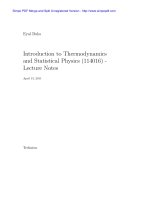
This result is know as Plank’s radiation law. The factor u
ω
represents th e
spectral distribution of the radiation. The peak in u
ω
is obtained at β~ω
0
=
2.82. I n terms of the wavelength λ
0
=2πc/ω
0
one has
λ
0
µm
=5.1
µ
T
1000 K
¶
−1
. (3.50)
0.2
0.4
0.6
0.8
1
1.2
1.4

0246810
x
The function x
3
/ (e
x
− 1).
The total energy is found by integrating Eq. (3.48) and by employing the
variable transformation x = β~ω
U
V
=
τ
4
c
3
π
2
~
3
∞
Z
0
x
3
dx
e
x
− 1
|

{z }
π
4
15
=
π
2
τ
4
15~
3
c
3
.
(3.51)
3.1.5 Stefan-Boltzmann Radiation La w
Consider a small hole having area dA drilled into the conductive wall of an
electromagnetic (EM) cavity. What is the rate of energy radiation emitted
from the hole? We employ below a kinetic approach to answer this question.
Considerradiationemittedinatimeintervaldt in the direction of the unit
vector ˆu.Letθ be th e angle between ˆu and the normal to the surface of the
hole. Photons emitted during that time interval dt in the direction ˆu came
from the region in the cavity that is indicated in Fig. 3.1, which has volume
Eyal Buks Thermodynamics and Statistical Physics 103
Chapter 3. Bosonic and Fermionic Systems
θ
dAcosθ
c
d
t

u
ˆ
θ
dAcosθ
c
d
t
u
ˆ
Fig. 3.1. Radiation emitted through a small hole in the cavity wall.
V
θ
=dA cos θ × cdt. (3.52)
The average energy in that region can be found using Eq. (3.51). Integrating
over all possible directions yields the total rate of energy radiation emitted
fromtheholeperunitarea
J =
1
dAdt
1
4π
π/2
Z
0
dθ sin θ
2π
Z
0
dϕ
U

V
V
θ
=
π
2
τ
4
15~
3
c
2
1
4π
π/2
Z
0
dθ sinθ cos θ
2π
Z
0
dϕ
|
{z }
1/4
=
π
2
τ
4

60~
3
c
2
(3.53)
In terms of the historical definition of temperature T = τ/k
B
[see Eq. (1.92)]
one has
J = σ
B
T
4
, (3.54)
where σ
B
,whichisgivenby
σ
B
=
π
2
k
4
B
60~
3
c
2
=5.67 × 10

−8
W
m
2
K
4
, (3.55)
is the Stefan-Boltzmann constant.
Eyal Buks Thermodynamics and Statistical Physics 104
3.2. Phonons in Solids
mm
ω
2
mm
ω
2
mm
ω
2
mm
ω
2
m
mm
ω
2
mm
ω
2
mm

ω
2
mm
ω
2
m
Fig. 3.2. 1D lattice.
3.2 Phonons in Solids
In this section we s tudy elastic waves in solids. We start w ith a one-
dimensional example, and then generalize some of the results for t he case
of a 3D lattice.
3.2.1 One Dimensional Example
Consider the 1D lattice show n in Fig. 3.2 below, which con tains N ’atoms’
having mass m eac h that are attac hed to each other by springs ha ving spring
constant mω
2
. The lattice spacing is a. The atoms are allowed to move in
one dimension along the array axis. In problem 5 of set 3 one finds that the
normal mode angular eigen-frequencies are given by
ω
n
= ω
p
2(1− cos k
n
a)=2ω
¯
¯
¯
¯

sin
k
n
a
2
¯
¯
¯
¯
, (3.56)
where a is the lattice spacing,
k
n
=
2πn
aN
, (3.57)
and n is in teger ranging from −N/2toN/2.
0
0.2
0.4
0.6
0.8
-1 -0.8 -0.6 -0.4 -0.2 0.2 0.4 0.6 0.8 1
x
The function |sin (πx/2)|.
Eyal Buks Thermodynamics and Statistical Physics 105
Chapter 3. Bosonic and Fermionic Systems
What is the partition function of an eigen-mode having eigen angular fre-
quency ω

n
? The mode amplitude has the dynamics of an harmonic oscillator
having angular frequency ω
n
. Thus, as we had in the previous section, where
we have discussed EM modes, the quantum eigenenergies of the mode are
ε
s
= s~ω
n
, (3 .58)
where s =0, 1, 2, is an integer. Wh en the mode is i n an eigenstate having
energy ε
s
the mode i s said to occupy s phonons. The c anonical partition
function of the m ode is found using Eq. (1.69)
Z
κ
=
∞
X
s=0
exp (−sβ~ω
κ
)
=
1
1 − exp (−β~ω
κ
)

.
(3.59)
Similarly to th e EM case, the average total energy is given by
U =
N/2
X
n=−N/2
}ω
n
exp (β}ω
n
) − 1
, (3.60)
where β =1/τ , and the total heat capacity is giv en by
C
V
=
∂U
∂τ
=
N/2
X
n=−N/2
(β}ω
n
)
2
exp (β}ω
n
)

[exp (β}ω
n
) − 1]
2
. (3 .61)
High Temperature Limit. In the high temperature limit β}ω ¿ 1
(β}ω
n
)
2
exp (β}ω
n
)
[exp (β}ω
n
) − 1]
2
' 1 , (3.62)
therefore
C
V
= N. (3.63)
Low Temperature Limit. In the low temperature limit β}ω À 1the
main contribution to the sum in Eq. (3.61) comes from terms for whic h
|n| . N/β}ω. Thus, to a good appro x imation the dispersion relation can be
approximated by
ω
n
=2ω
¯

¯
¯
¯
sin
k
n
a
2
¯
¯
¯
¯
' 2ω
¯
¯
¯
¯
k
n
a
2
¯
¯
¯
¯
= ω
2π
N
|n| . (3.64)
Moreover, in the limit N À 1thesuminEq.(3.61)canbeapproximated

by an integral, a nd to a good approximation the upper limit N/2canbe
substituted by infinity, thus
Eyal Buks Thermodynamics and Statistical Physics 106
3.2. Phonons in Solids
C
V
=
N/2
X
n=−N/2
(β}ω
n
)
2
exp (β}ω
n
)
[exp (β}ω
n
) − 1]
2
' 2
∞
X
n=0
¡
β}ω
2π
N
n

¢
2
exp
¡
β}ω
2π
N
n
¢
£
exp
¡
β}ω
2π
N
n
¢
− 1
¤
2
' 2
Z
∞
0
dn
¡
β}ω
2π
N
n

¢
2
exp
¡
β}ω
2π
N
n
¢
£
exp
¡
β}ω
2π
N
n
¢
− 1
¤
2
=
N
π
τ
}ω
Z
∞
0
dx
x

2
exp (x)
(exp (x) − 1)
2
| {z }
π
2
/3
=
Nπ
3
τ
}ω
.
(3.65)
3.2.2 The 3D Case
The case of a 3D lattice is similar t o the case of EM cavity that we have
studied in the previous section. Ho wev er, there are 3 importan t distinctions:
1. The number of modes of a lattice containing N atoms that can move in
3D is finite, 3N instead of infinity as in the EM case.
2. For any given v ector k there are 3, instead of only 2, orthogonal modes
(polarizations).
3. Dispersion: contrary to the EM case, the dispersion relation (namely, the
function ω (k)) is in general nonlinea r.
Due to distinctions 1 and 2 , the sum ov er all modes is substituted by an
integral according to
∞
X
n
x

=0
∞
X
n
y
=0
∞
X
n
z
=0
→
3
8
4π
n
D
Z
0
dnn
2
, (3 .66)
where the factor of 3 replaces the factor of 2 we had in the EM case. Moreover,
the upper limit is n
D
instead o f infinity, where n
D
is determined from the
requirement
3

8
4π
n
D
Z
0
dnn
2
=3N, (3.67)
thus
n
D
=
µ
6N
π
¶
1/3
. (3.68)
Eyal Buks Thermodynamics and Statistical Physics 107
Chapter 3. Bosonic and Fermionic Systems
Similarly to th e EM case, the average total energy is given by
U =
X
n
}ω
n
exp (β}ω
n
) − 1

(3.69)
=
3π
2
n
D
Z
0
dnn
2
}ω
n
exp (β}ω
n
) − 1
.
(3.70)
To proceed with the calculation the dispersion relation ω
n
(k
n
) is needed.
Here we assume for simplicity that dispersion can be disregarded to a good
approximation, and consequently the dispersion relation can be assumed to
be linear
ω
n
= vk
n
, (3.71)

where v is the sound velocity. The wave vector k
n
is related to n =
q
n
2
x
+ n
2
y
+ n
2
z
by
k
n
=
πn
L
, (3.72)
where L = V
1/3
and V is the volume. In this approximation one finds using
the variable transformation
x =
β}vπn
L
, (3.73)
that
U =

3π
2
n
D
Z
0
dnn
2
}vπn
L
exp
³
β}vπn
L
´
− 1
=
3Vτ
4
2}
3
v
3
π
2
x
D
Z
0
dx

x
3
exp x − 1
.
(3.74)
where
x
D
=
β}vπn
D
L
=
β}vπ
¡
6N
π
¢
1/3
L
.
Alternatively, in terms of the Debye temperature, which is defined as
Θ = }v
µ
6π
2
N
V
¶
1/3

, (3.75)
one has
Eyal Buks Thermodynamics and Statistical Physics 108
3.2. Phonons in Solids
x
D
=
Θ
τ
, (3.76)
and
U =9Nτ
³
τ
Θ
´
3
x
D
Z
0
dx
x
3
exp x − 1
. (3.77)
As an example Θ/k
B
= 88 K for Pb, while Θ/k
B

= 1860 K f or diamond.
Below we calculate the heat capacity C
V
= ∂U/∂τ in two limits.
High Temperature Limit. In the high tem perature limit x
D
= Θ/τ ¿ 1,
thus
U =9Nτ
³
τ
Θ
´
3
x
D
Z
0
dx
x
3
exp x −1
' 9Nτ
³
τ
Θ
´
3
x
D

Z
0
dxx
2
=9Nτ
³
τ
Θ
´
3
x
3
D
3
=3Nτ ,
(3.78)
and therefore
C
V
=
∂U
∂τ
=3N. (3.79)
Note that in this limit the averag e energy of each mode is τ and consequently
U =3Nτ. This result dem onstrates the equal partition theorem of classical
statistical mechanics that will be discussed in the next c hapter.
Low Temperature Limit. In the low temperature limit x
D
= Θ/τ À 1,
thus

U =9Nτ
³
τ
Θ
´
3
x
D
Z
0
dx
x
3
exp x −1
' 9Nτ
³
τ
Θ
´
3
∞
Z
0
dx
x
3
exp x − 1
|
{z }
π

4
/15
=
3π
4
5
Nτ
³
τ
Θ
´
3
,
(3.80)
Eyal Buks Thermodynamics and Statistical Physics 109
Chapter 3. Bosonic and Fermionic Systems
and therefore
C
V
=
∂U
∂τ
=
12π
4
5
N
³
τ
Θ

´
3
. (3.81)
Note that Eq. (3.80) together w ith Eq. (3.75) yield
U
V
=
3
2
π
2
τ
4
15}
3
v
3
. (3.82)
Note the similarity between this result and Eq. (3.51) for the EM case.
3.3 Fermi Gas
In this section we study an ideal gas of Fermions of mass m. While o n ly the
classical limit was considered in chapter 2, here we consider the more general
case.
3.3.1 Orbital Partition Function
Consider an orbital having energy ε
n
. Disregarding internal degrees of free-
dom, its g randcanonical Fermionic partition function is given by [see Eq.
(2.33)]
ζ

n
=1+λ exp (−βε
n
) , (3.83)
where
λ =exp(βµ)=e
−η
, (3.84)
is the fugacity and β =1/τ . Taking into account internal degrees of freedom
the grandcanonical Fermionic partition function becomes
ζ
n
=
Y
l
(1 + λ exp( −βε
n
)exp(−βE
l
)) , (3.85)
where {E
l
} are the eigenenergies of a particle due to internal degrees of
freedom [see Eq. (2.71)]. As is required by the Pauli exclusion principle, no
more than one Fermion can occupy a given internal eigenstate and a giv en
orbital.
3.3.2 Partition Function of the Gas
The grandcanonical partition function of the gas is given b y
Z
gc

=
Y
n
ζ
n
. (3.86)
Eyal Buks Thermodynamics and Statistical Physics 110
3.3. Fermi Gas
As we have seen in chapter 2, the orbital eigenenergies of a particle of mass
m in a bo x are given b y Eq. (2.5)
ε
n
=
~
2
2m
³
π
L
´
2
n
2
, (3.87)
where
n =(n
x
,n
y
,n

z
) , (3.88)
n =
q
n
2
x
+ n
2
y
+ n
2
z
, (3.89)
n
x
,n
y
,n
z
=1, 2, 3, , (3.90)
and L
3
= V is the volume of the box. Th us, log Z
gc
can be written as
log Z
gc
=
∞

X
n
x
=1
∞
X
n
y
=1
∞
X
n
z
=1
log ζ
n
. (3.91)
Alternatively, using t he notation
α
2
=
β~
2
π
2
2mL
2
, (3.92)
and Eq. (3.85) one has
log Z

gc
=
X
l
∞
X
n
x
=1
∞
X
n
y
=1
∞
X
n
z
=1
log
¡
1+λ exp
¡
−α
2
n
2
¢
exp (−βE
l

)
¢
. (3.93)
For a macroscopic system α ¿ 1, and consequen tly the sum over n can
be appro x imately replaced by an integral
∞
X
n
x
=0
∞
X
n
y
=0
∞
X
n
z
=0
→
1
8
4π
∞
Z
0
dnn
2
, (3.94)

thus, one has
log Z
gc
=
π
2
X
l
∞
Z
0
dnn
2
log
¡
1+λ exp
¡
−α
2
n
2
¢
exp (−βE
l
)
¢
. (3.95)
This can be further simplified by employing the variable transformation
βε = α
2

n
2
. (3.96)
The following holds
Eyal Buks Thermodynamics and Statistical Physics 111