Introduction to Thermodynamics and Statistical Physics phần 8 ppt
Bạn đang xem bản rút gọn của tài liệu. Xem và tải ngay bản đầy đủ của tài liệu tại đây (255.59 KB, 17 trang )
Chapter 3. Boso nic and Fermionic Systems
√
ε
2
µ
β
α
2
3/2
dε = n
2
dn.
Thus, b y introducing the densityofstates
D (ε)=
(
V
2π
2
¡
2m
~
2
¢
3/2
ε
1/2
ε ≥ 0
0 ε<0
, (3.97)
one has
log Z
gc
=
1
2
X
l
∞
Z
−∞
dεD(ε)log(1+λ exp (−β (ε + E
l
))) . (3.98)
3.3.3 Energy and Number of Particles
Using Eqs. (1.80) a nd (1.94) for the energy U and the number of particles
N,namelyusing
U = −
µ
∂ log Z
gc
∂β
η
, (3.99)
N = λ
∂ logZ
gc
∂λ
, (3.100)
one finds that
U =
1
2
X
l
∞
Z
−∞
dεD(ε)(ε + E
l
) f
FD
(ε + E
l
) , (3.101)
N =
1
2
X
l
∞
Z
−∞
dεD(ε) f
FD
(ε + E
l
) , (3.102)
where f
FD
is the Fermi-Dirac distribution function [see Eq. (2.35)]
f
FD
()=
1
exp [β ( − µ)] + 1
. (3.103)
3.3.4 Example: Electrons in Metal
Electrons are Fermions having spin 1/2. The spin degree of freedom gives rise
to two orthogo nal eigenstates having energies E
+
and E
−
respectively. In the
absent of any external magnetic field these states are degenerate, namely
E
+
= E
−
. For simplicity we take E
+
= E
−
= 0. Thus, Eqs. (3.101) and
(3.102) become
Eyal Buks Thermodynamics and Statistical Physics 112
3.3. Fermi Gas
U =
∞
Z
−∞
dεD(ε) εf
FD
(ε) , (3.104)
N =
∞
Z
−∞
dεD(ε) f
FD
(ε) , (3.105)
T ypically f or metals at room temperature or below the following holds τ ¿ µ.
Thus, it is c onvenien t to employ the following theorem ( Sommerfeld expan-
sion) to evaluate these integrals.
Theorem 3.3.1. Let g (ε) be a function that vanishes in the limit ε →−∞,
and that diverges no more rapidly than some p ower of ε as ε →∞.Then,
the following holds
∞
Z
−∞
dεg(ε) f
FD
(ε)
=
µ
Z
−∞
dεg(ε)+
π
2
g
0
(µ)
6β
2
+ O
µ
1
βµ
4
.
Proof. See problem 7 of set 3.
With the help of this theorem the n umber of particles N to second order
in τ is given by
N =
µ
Z
−∞
dεD(ε)+
π
2
τ
2
D
0
(µ)
6
. (3.106)
Moreover, at low temperatures, the chemical potential is expected to be close
the the Fermi energy ε
F
, which is defined by
ε
F
= lim
τ→0
µ. (3.107)
Thus, to lowest order in µ − ε
F
one has
µ
Z
−∞
dεD(ε)=
ε
F
Z
−∞
dεD(ε)+(µ − ε
F
) D (ε
F
)+O (µ − ε
F
)
2
, (3.108)
and therefore
N = N
0
+(µ −ε
F
) D (ε
F
)+
π
2
τ
2
D
0
(ε
F
)
6
, (3.109)
where
Eyal Buks Thermodynamics and Statistical Physics 113
Chapter 3. Boso nic and Fermionic Systems
N
0
=
ε
F
Z
−∞
dεD(ε) , (3.110)
is the number of electrons at zero temperature. The number of electrons N
in metals is expected to be temperature independent, namely N = N
0
and
consequently
µ = ε
F
−
π
2
D
0
(ε
F
)
6β
2
D (ε
F
)
. (3.111)
Similarly, the energy U at low temperatures is given approximat ely by
U =
∞
Z
−∞
dεD(ε) εf
FD
(ε)
=
ε
F
Z
−∞
dεD(ε) ε
|
{z }
U
0
+(µ −ε
F
) D (ε
F
) ε
F
+
π
2
τ
2
6
(D
0
(ε
F
) ε
F
+ D (ε
F
))
= U
0
−
π
2
τ
2
D
0
(ε
F
)
6D (ε
F
)
D (ε
F
) ε
F
+
π
2
τ
2
6
(D
0
(ε
F
) ε
F
+ D (ε
F
))
= U
0
+
π
2
τ
2
6
D (ε
F
) ,
(3.112)
where
U
0
=
ε
F
Z
−∞
dεD(ε) ε. (3.113)
From this result one finds that the e lectronic heat capacity is given by
C
V
=
∂U
∂τ
=
π
2
τ
3
D (ε
F
) . (3.114)
Comparing this result with Eq. (3.81) fo r the phonons heat capacity, which
is proportional to τ
3
at low temperatures, suggests that typically, while the
electronic contribution is the dominant one at very low temperatures, at
higher te mperatures the phonons’ contribution becomes dominant.
3.4 Semiconductor Statistics
To be written
Eyal Buks Thermodynamics and Statistical Physics 114
3.5. Problems Set 3
3.5 Problems Set 3
1. Calculate the average number of photons N in equilibrium at tempera-
ture τ in a cavity of volum e V . Use this result to estimate the number
of photons in the universe assuming it to be a spherical cavity of radius
10
26
m and at temperature τ = k
B
× 3K.
2. Write a relation between the temperature of the surface of a planet and its
distance from the Sun, on the assumption that as a black body in thermal
equilibrium, it rera d iates as much thermal radiation, as it receives from
the Sun. Assume also, that the surface of the planet is at constant temper-
ature over the day-nigh t cycle. Use T
Sun
=5800K;R
Sun
=6.96 × 10
8
m;
and the Mars-Sun distance of D
M−S
=2.28 × 10
11
m and calculate the
temperature of M ars surface.
3. Calculate the Helmholtz free energy F of photon gas having total e nergy
U and volume V and use your result to show that the pressure is given
by
p =
U
3V
. (3.115)
4. Consider a photon gas initially at temperature τ
1
and volume V
1
.Thegas
is adiabatically compressed from volume V
1
to volume V
2
in an isentropic
process. Calculate the final temperature τ
2
and final p ressure p
2
.
5. Consider a one-dimensional lattice of N iden tical point particles of mass
m, int eracting via nearest-neighbor spring-like forces with spring constant
mω
2
(see Fig. 3.2). Denote the lattice spacing by a. Show that the normal
mode eigen-frequencies are given b y
ω
n
= ω
p
2(1− cos k
n
a) , (3.116)
where k
n
=2πn/aN,andn is in teger r anging from −N/2toN/2 (assume
N À 1).
6. Consider an orbital with energy ε in an ideal gas. The system is in thermal
equilibrium at temperature τ and chemical potential µ.
a) Show that the probability t hat the orbital is occupied by n particles
is given by
p
F
(n)=
exp [n (µ − ε) β]
1+exp[(µ − ε) β]
, (3.117)
for the c ase of Fermions, w here n ∈ {0, 1},andby
p
B
(n)={1 − exp [(µ − ε) β]} exp [n (µ − ε) β] , (3.118)
where n ∈ {0, 1, 2, }, for the case of Bosons.
Eyal Buks Thermodynamics and Statistical Physics 115
Chapter 3. Boso nic and Fermionic Systems
b) Sho w that the variance (∆n)
2
=
D
(n − hni)
2
E
is given by
(∆n)
2
F
= hni
F
(1 − hni
F
) , (3.119)
for the c ase of Fermions, and by
(∆n)
2
B
= hni
B
(1 + hni
B
) , (3.120)
for the case of Bosons.
7. Let g (ε) be a function that vanishes in the limit ε →−∞,andthat
diverges no more rapidly than some pow er of ε as ε →∞. Show that the
following holds (Sommerfeld expansion)
I =
∞
Z
−∞
dεg(ε) f
FD
(ε)
=
µ
Z
−∞
dεg(ε)+
π
2
g
0
(µ)
6β
2
+ O
µ
1
βµ
4
.
8. Cons ider a metal at zero temperature having Ferm i e nergy ε
F
,number
of electrons N and v olume V .
a) Calculate the mean en ergy of electrons.
b) Calculate the ratio α of the mean-square- speed of electrons to the
square of the mean s peed
α =
v
2
®
hvi
2
. (3.121)
c) Calculate the pressure exerted by an electr on gas at zero tempera-
ture.
9. For electrons with energy ε À mc
2
(relativistic fermi gas), the energy
is given by ε = pc. Find the fermi energy of this gas and show that the
ground state energy is
E (T =0)=
3
4
Nε
F
(3.122)
10. A gas of two dimensional electrons is free to mo ve in a p lane. The mass
of each electron is m
e
, the density (number of electrons per unit area) is
n,andthetemperatureisτ. Show that the chemical potential µ is given
by
µ = τ log
·
exp
µ
nπ~
2
m
e
τ
− 1
¸
. (3.123)
Eyal Buks Thermodynamics and Statistical Physics 116
3.6. Solutions Set 3
3.6 Solutions Set 3
1. The density of states of the photon gas is giv en b y
dg =
Vε
2
π
2
}
3
c
3
dε. (3.124)
Thus
N =
V
π
2
}
3
c
3
∞
Z
0
ε
2
e
ε/τ
− 1
dε
= V
³
τ
}c
´
3
α, (3.125)
where
α =
1
π
2
∞
Z
0
x
2
e
x
− 1
dx. (3.126)
The number α is calculated numerically
α =0.24359 . (3.127)
For the universe
N =
4π
3
¡
10
26
m
¢
3
µ
1.3806568 × 10
−23
JK
−1
3K
1.05457266 × 10
−34
Js2.99792458 × 10
8
ms
−1
3
× 0.24359
' 2.29 × 10
87
. (3.128)
2. The energy emitted by the Sun is
E
Sun
=4πR
2
Sun
σ
B
T
4
Sun
, (3.129)
and the energy emitte d by a planet is
E
planet
=4πR
2
planet
σ
B
T
4
planet
. (3.130)
The fraction of Sun energy that pla net receives is
πR
2
planet
4πD
2
M−S
E
Sun
, (3.131)
and this e quals to the energy it reradiates. Therefore
πR
2
planet
4πD
2
E
Sun
= E
planet
,
Eyal Buks Thermodynamics and Statistical Physics 117
Chapter 3. Boso nic and Fermionic Systems
thus
T
planet
=
r
R
Sun
2D
T
Sun
,
and for Mars
T
Mars
=
r
6.96 × 10
8
m
2 × 2.28 × 10
11
m
5800 K = 226 K .
3. The partition function is giv en by
Z =
Y
n
∞
X
s=0
exp (sβ}ω
n
)=
Y
n
1
1 − exp (−β}ω
n
)
,
th us the free energy is given by
F = −τ log Z = τ
X
n
log [1 − exp (−β}ω
n
)] .
Transforming the sum over modes into integral yields
F = τπ
Z
∞
0
dnn
2
log [1 − exp (−β}ω
n
)] (3.132)
= τπ
Z
∞
0
dnn
2
log
·
1 − exp
µ
−
β}πcn
L
¶¸
,
or, by integrating by parts
F = −
1
3
}π
2
c
L
Z
∞
0
dn
n
3
exp
³
β}πcn
L
´
− 1
= −
1
3
U,
where
U =
π
2
τ
4
V
15}
3
c
3
. (3.133)
Thus
p = −
µ
∂F
∂V
τ
=
U
3V
. (3.134)
4. Using the expression for Helmholtz free energy, which was derived in the
previous problem,
F = −
U
3
= −
π
2
τ
4
V
45}
3
c
3
,
one finds that the en tropy is given by
Eyal Buks Thermodynamics and Statistical Physics 118
3.6. Solutions Set 3
σ = −
µ
∂F
∂τ
V
=
4π
2
τ
3
V
45}
3
c
3
.
Thus, for an isentropic process, for which σ is a constant, one has
τ
2
= τ
1
µ
V
1
V
2
1/3
.
Using again the previous problem, the pressure p is given by
p =
U
3V
,
thus
p =
π
2
τ
4
45}
3
c
3
,
and
p
2
=
π
2
τ
4
1
45}
3
c
3
| {z }
p
1
µ
V
1
V
2
4/3
.
5. Let u (na) be the displacement of poin t p article number n. The equations
of motion are given by
m¨u (na)=−mω
2
{2u (na) − u [(n − 1) a] − u [(n +1)a]} . (3.135)
Consider a s olution of the form
u (na, t)=e
i(kna−ω
n
t)
. (3.136)
P eriodic boundary condition requires that
e
ikNa
=1, (3.137)
thus
k
n
=
2πn
aN
. (3.138)
Substituting in Eq. 3.135 yields
−mω
2
n
u (na)=−mω
2
£
2u (na) − u (na) e
−ika
− u (na) e
ika
¤
, (3.139)
or
ω
n
= ω
p
2(1− cos k
n
a)=2ω
¯
¯
¯
¯
sin
k
n
a
2
¯
¯
¯
¯
. (3.140)
Eyal Buks Thermodynamics and Statistical Physics 119
Chapter 3. Boso nic and Fermionic Systems
6. In general using Gibbs factor
p (n)=
exp [n (µ − ε) β]
X
n
0
exp [n
0
(µ − ε) β]
, (3.141)
where β =1/τ ,onefinds for Fermions
p
F
(n)=
exp [n (µ − ε) β]
1+exp[(µ − ε) β]
, (3.142)
where n ∈ {0, 1},andforBosons
p
B
(n)=
exp [n (µ − ε) β]
∞
X
n
0
=0
exp [n
0
(µ − ε) β]
= {1 − exp [(µ − ε) β]} exp [ n (µ − ε) β] ,
(3.143)
where n ∈ {0, 1, 2, }. The expectation value of hni in general is given
by
hni =
X
n
0
n
0
p (n
0
)=
X
n
0
n
0
exp [n (µ − ε) β]
X
n
0
exp [n
0
(µ − ε) β]
, (3.144)
thus for Fermions
hni
F
=
1
exp [(ε − µ) β]+1
, (3.145)
and for Bosons
hni
B
= {1 − exp [(µ − ε) β]}
∞
X
n
0
=0
n
0
exp [n
0
(µ − ε) β]
= {1 − exp [(µ − ε) β]}
exp [(µ − ε) β]
(1 − exp [(µ − ε) β])
2
=
1
exp [(ε −µ) β] − 1
.
(3.146)
In general, the following holds
τ
µ
∂ hni
∂µ
τ
=
X
n
00
(n
00
)
2
exp [n (µ − ε) β]
X
n
0
exp [n
0
(µ − ε) β]
−
X
n
0
n
0
exp [n
0
(µ − ε) β]
X
n
0
exp [n
0
(µ − ε) β]
2
=
n
2
®
− hni
2
=
D
(n − hni)
2
E
.
(3.147)
Eyal Buks Thermodynamics and Statistical Physics 120
3.6. Solutions Set 3
Thus
(∆n)
2
F
=
exp [(ε − µ) β]
(exp [( ε − µ) β]+1)
2
= hni
F
(1 − hni
F
) , (3.148)
(∆n)
2
B
=
exp [(ε − µ) β]
(exp [( ε − µ) β] − 1)
2
= hni
B
(1 + hni
B
) . (3.149)
7. Let
G (ε)=
ε
Z
−∞
dε
0
g (ε
0
) . (3.150)
Integration by parts yields
I =
∞
Z
−∞
dεg(ε) f
FD
(ε)
=[G (ε) f
FD
(ε)|
∞
−∞
| {z }
=0
+
∞
Z
−∞
dεG(ε)
µ
−
∂f
FD
∂ε
,
(3.151)
where the fo llowing holds
µ
−
∂f
FD
∂ε
=
βe
β(ε−µ)
¡
e
β(ε−µ)
+1
¢
2
=
β
4cosh
2
³
β
2
(ε − µ)
´
. (3.152)
Using the Taylor expansion of G ( ε)aboutε −µ, which has the form
G (ε)=
∞
X
n=0
G
(n)
(µ)
n!
(ε − µ)
n
, (3.153)
yields
I =
∞
X
n=0
G
(n)
(µ)
n!
∞
Z
−∞
β (ε − µ)
n
dε
4cosh
2
³
β
2
(ε − µ)
´
. (3.154)
Employing the variable transformation
x = β (ε − µ) , (3.155)
and exploiting the fact that (−∂f
FD
/∂ε)isanevenfunctionofε−µ leads
to
Eyal Buks Thermodynamics and Statistical Physics 121
Chapter 3. Boso nic and Fermionic Systems
I =
∞
X
n=0
G
(2n)
(µ)
(2n)!β
2n
∞
Z
−∞
x
2n
dx
4cosh
2
x
2
. (3.156)
With the help of the identities
∞
Z
−∞
dx
4cosh
2
x
2
=1, (3.157)
∞
Z
−∞
x
2
dx
4cosh
2
x
2
=
π
2
3
, (3.158)
one finds
I = G (µ)+
π
2
G
(2)
(µ)
6β
2
+ O
µ
1
βµ
4
=
µ
Z
−∞
dεg(ε)+
π
2
g
0
(µ)
6β
2
+ O
µ
1
βµ
4
.
(3.159)
8. In general, at ze ro temperature the average of the energy ε to the power
n is given by
hε
n
i =
ε
F
R
0
dεD(ε) ε
n
ε
F
R
0
dεD(ε)
, (3.160)
where D (ε) is the density of states
D (ε)=
V
2π
2
µ
2m
~
2
3/2
ε
1/2
, (3.161)
thus
hε
n
i =
ε
n
F
2n
3
+1
. (3.162)
a) Using Eq. (3.162) one finds that
hεi =
3ε
F
5
. (3.163)
b) The speed v is related to the energy by
v =
r
2ε
m
, (3.164)
Eyal Buks Thermodynamics and Statistical Physics 122
3.6. Solutions Set 3
thus
α =
hεi
ε
1/2
®
2
=
ε
F
2
3
+1
¿
ε
−1/2
F
2
3
1
2
+1
À
2
=
16
15
. (3.165)
c) T he number of electrons N is giv en by
N =
ε
F
Z
0
dεD(ε)=
D (ε
F
)
ε
1/2
F
ε
F
Z
0
dεε
1/2
=
D (ε
F
)
ε
1/2
F
2
3
ε
3/2
F
,
thus
ε
F
=
~
2
2m
µ
3π
2
N
V
2/3
, (3.166)
and therefore
U =
3N
5
~
2
2m
µ
3π
2
N
V
2/3
. (3.167)
Moreover, at zero temperature the Helmho ltz free energy F = U −
τσ = U,thusthepressureisgivenby
p = −
µ
∂F
∂V
τ,N
= −
µ
∂U
∂V
τ,N
=
3N
5
~
2
2m
µ
3π
2
N
V
2/3
2
3V
=
2Nε
F
5V
.
(3.168)
9. The energy of the particles are
ε
n,±
= pc (3.169)
where p = ~k, and k =
πn
L
,n=
q
n
2
x
+ n
2
y
+ n
2
z
and n
i
=1, 2,
Therefore
N =2×
1
8
×
4
3
πn
3
F
=
π
3
n
3
F
(3.170)
n
F
=
µ
3N
π
1/3
ε
F
=
~cπ
L
µ
3N
π
1/3
= ~cπ
µ
3N
πV
1/3
Eyal Buks Thermodynamics and Statistical Physics 123
Chapter 3. Boso nic and Fermionic Systems
The energy is given by
E (T =0)=
ε
F
Z
0
εg (ε) dε =
L
3
π
2
~
3
c
3
Z
ε
F
0
ε
3
dε = (3.171)
=
L
3
π
2
~
3
c
3
×
ε
4
F
4
=
1
4
L
3
π
2
~
3
c
3
ε
3
F
× ε
F
=
=
1
4
L
3
π
2
~
3
c
3
3π
2
~
3
c
3
N
L
3
ε
F
=
3
4
Nε
F
10. The energy of an electron having a wave f unction proportional to exp (ik
x
x)exp(ik
y
y)
is
~
2
2m
e
¡
k
2
x
+ k
2
y
¢
. (3.172)
For periodic boundary conditions one has
k
x
=
2πn
x
L
x
, (3.173)
k
y
=
2πn
y
L
y
, (3.174)
where the sample is of area L
x
L
y
,andn
x
and n
y
are both integers. The
number of states having energy smaller th an E
0
is given by (including
both spin directions)
2π
2m
e
E
0
~
2
L
x
L
y
4π
2
, (3.175)
th us, the density of state per unit area is given by
D (E)=
½
m
e
π~
2
E>0
0 E<0
. (3.176)
Using Fermi-Dirac function
f (E)=
1
1+exp[β (E − µ)]
, (3.177)
where β =1/τ , the density n is giv en by
n =
Z
∞
−∞
D (E) f (E)dE
=
m
e
π~
2
Z
∞
0
dE
1+exp[β (E − µ)]
=
m
e
τ
π~
2
log
¡
1+e
βµ
¢
,
(3.178)
Eyal Buks Thermodynamics and Statistical Physics 124
3.6. Solutions Set 3
thus
µ = τ log
·
exp
µ
nπ~
2
m
e
τ
− 1
¸
. (3.179)
Eyal Buks Thermodynamics and Statistical Physics 125
4. Classical Limit of Statistical Mechanics
In this chapter we discuss the classical limit of statistical m echanics. We dis-
cuss Hamilton’s formalism, define the Hamiltonian and present t he Hamilton-
Jacobi equations of motion. The density function in thermal equilibrium is
used to pro ve t he e quipartition theorem. This theorem is then employed to
analyze an electrical circuit in ther mal equilibrium, and to calculate voltage
noise across a resistor (Nyquist noise formula).
4.1 Classical H amiltonian
In this section we briefly review Hamilton’s formalism, which is analogous to
Newton’s laws of classical m echanics . Consider a classical system having d
degrees of freedom. T he system is described using the vector o f coordinates
¯q =(q
1
,q
2
, , q
d
) . (4.1)
Let E be the total energy o f th e system. For simplicity we restrict the dis-
cussion to a special case where E isasumoftwoterms
E = T + V,
where T depends only on velocities, namely T = T
³
·
¯q
´
,andwhereV depends
only on coordinates, namely V = V (¯q). T he notation overdot i s used to
express time derivative, namely
·
¯q =
µ
dq
1
dt
,
dq
2
dt
, ,
dq
d
dt
. (4.2)
We refer to the first term T as kinetic e nergy and to the second one V as
potential energy.
The canonical conjugate momentum p
i
of the coordinate q
i
is defined as
p
i
=
∂T
∂ ˙q
i
. (4.3)
The c lassical Hamiltonian H of the system is expressed as a function of the
vector of coordinates ¯q and as a function of the vector of canonical conjugate
momentum variables
Chapter 4. Classical Limit of Statistical Mechanics
¯p =(p
1
,p
2
, , p
d
) , (4.4)
namely
H = H (¯q, ¯p) , (4.5)
and it is defined by
H =
d
X
i=1
p
i
˙q
i
− T + V. (4.6)
4.1.1 Hamilton-Jacobi Equations
The equations of motion of the system are given by
˙q
i
=
∂H
∂p
i
(4.7)
˙p
i
= −
∂H
∂q
i
, (4.8)
where i =1, 2, d.
4.1.2 Ex ample
q
V(q)
m
q
V(q)
m
Consider a pa rticle having mass m in a one dime nsional potential V (q).
The kinetic energy is given by T = m ˙q
2
/2, thus the canonical conjugate mo-
mentum is given by [see Eq. (4.3)] p = m ˙q. Th u s for this example t he canon-
ical conjugate momentum equals the mechanical momentum. Note, however,
that this is not necessarily always the case. Using the d efinition (4.6) one
finds that the Hamiltonian is giv en by
Eyal Buks Thermodynamics and Statistical Physics 128