Engineering Drawing for Manufacture phần 7 pptx
Bạn đang xem bản rút gọn của tài liệu. Xem và tải ngay bản đầy đủ của tài liệu tại đây (883.23 KB, 17 trang )
96
Engineering drawing for manufacture
Tolerance band width
- 0,021
Tolerance
band f7 = .o,o~,
-o.o2o
f7 =-o.o41
Lower size limit for
f7 (19.959) ] I Go-NoGo
Gauge
r- ~ r" ~ r" r" t- r" ~ r-
J I
tt
test
Figure 5.8
Example of a 20,00f7 go~no-go gauge inspecting 10 shafts from a
production line
5.4.1 Fit systems
Figure 5.9 shows the three basic fit 'systems'. The left-hand sketch
shows a shaft which will always fit in the hole because the shaft
maximum size is always smaller than the hole minimum size. This is
called a
clearance fit.
These have been discussed above with respect
to running and sliding fits as per Figure 5.1. In some functional
performance situations, an
interferencefit
is required. In this case, the
shaft is always larger than the hole. This would be the case for the
piston rings prior to their assembly within an engine bore or for a
hub on a shaft. In some functional performance situations, a
tran-
sition fit
may be required. Should the shaft and hole final diameters
be an interference-clearance fit, the clearances will be very small
and the location would be very accurate. If it were an interference-
transition fit, on assembly the shaft would 'shave' the hole and thus
the location would be very accurate.
5.4.2 The "shaft basis" and the "hole basis' system of fits
In all the examples given above, the discussion has been concerning
'shafts' and 'holes'. It should be remembered that this does not
necessarily apply to shafts and holes. These are just generic terms
that mean anything that fits inside anything else. However,
whatever the case, it is often the case that either the shaft or the hole
is the easier to produce. For example, if they are cylindrical, the
shaft will be the more easily produced in that one turning tool can
produce an infinite number of shaft diameters. This is not the case
with the cylindrical hole in that each hole size will be dependent on
a single drill or reamer.
Limits, fits and geometrical tolerancing
97
p_8
,J
:.:.:;:.:.:.:.:.:.:.:.:.:.:.:.:.:
.:.:-:,:-:.:o:
9 -!
E ~: ~
-r -r
i Clearance Fit I
I[ Transition Fit I
#
#
~ / Interference Fit I
Figure
5.9
Typical clearance, transition and interference fits for a shaft in a hole
DIFFERENT SHAFTS ~-
._o =~
Range of
different
shaft
tolerance
sizes
i Hole basis I
system of fits. I
DIFFERENT HOLES
~|
Range of
different
tolerance
sizes
IL Clearancefi, ~kmnsitionftlt InJterferencef~it I
Shaft
basis
system of fits.
Figure 5.10
Hole basis and shaft basis examples of fits
The right-hand diagram in Figure 5.10 shows the situation in
which the shaft is the more difficult of the two to produce and this is
referred to as the 'shaft basis' system of fits. In this case the system of
fits is used in which the required clearances or interferences are
obtained by associating holes of various tolerance classes with shafts
of a single tolerance class. Alternatively if the shaft is the easier part
to produce then the hole basis system of fits is used. This is a system
of fits in which the required clearances and interferences are
obtained by associating shafts of various tolerance classes with holes
of a single tolerance class. In the case of the shaft basis system the
shaft is kept constant and the interference or clearance functional
situation is achieved by manipulating the hole. If the hole-based
98
Engineering drawing for manufacture
system is used, the opposite is the case. The appropriate use of each
system for functional performance situation is thus made easier for
the manufacturer.
5.4.3 Fit types and categories
Clearance fits can be subdivided into running or sliding fits.
Running applies to a shaft rotating at speed within a journal
whereas sliding can be represented by slow translation, typically of a
spool valve. Running and sliding fits are intended to provide a
similar running performance with suitable lubrication allowance
throughout a range of sizes. Transition fits are used for locational
purposes. Because of the difference in sizes they will either be low
clearance fits or low interference fits. They are intended to provide
only the location of mating parts. They may provide rigid or
accurate location as with interference fits or provide some measure
of freedom in location as in small clearance fits. Interference fits are
normally divided into force or shrink fits. These constitute a special
type of interference. The idea of the interference is to create an
internal stress that is constant through a range of sizes because the
interference varies with diameter. The resulting residual stress
caused by the interference will be dictated by the functional
performance situation.
From the data given above it should be fairly obvious that there is
a massive number of permutations of fits and classes and sizes. This
begs the question, how does a designer select a particular one from
the multitude available? The answer is that designers use a
preferred set of fits. Many examples of preferred fits are available.
Examples of commonly used ones are given in the standards BS
4500A and BS 4500B re British practice. The charts of preferred fits
given in Figures 5.11 and 5.12 are a subset of the BS 4500 selection.
Although these eight classes are just a selection, they represent
archetypal cases. Regarding clearance fits, the loose running fit class
is for wide commercial tolerances or allowances. The free running
fit is not for use where accuracy is essential but is appropriate for
large temperature variations, high running speeds or heavy journal
pressures. The close running fit is for running on accurate machines
or for accurate location at moderate speeds and journal pressures.
The sliding fit is not intended to run freely but to move and turn
freely and locate accurately. The low locational transition fit is
for accurate location and is a compromise between clearance and
Limits, fits and geometrical tolerancing
99
interference. The high locational transition fit is for more accurate
location where greater interference is permissible. The locational
interference fit is for parts requiring rigidity and alignment with the
prime accuracy of location but without any special residual pressure
requirement. The medium drive fit is for ordinary steel parts or
shrink fits on light sections. It is the tightest fit useable with cast
iron. These eight classes provide a useful starting point for most
functional performance situations.
Selected ISO fits for the 'hole basis' system (all values in urn)
+200um
Hll ~
+100um ~
~,z'_
H8 H7 H7 H7 Izzz~ i p~ r77~ 17"~6
,
_ [~
~7~ ~-z~ ~ / ~z-~_o i
~
_ _ _ ~
f7 ~ trr~
g6 k6 I ' " ,,ii
-100um ~ ~
9
l
-20oum ~ ~ ~ Tolerances on diagram to scale for range 18 to 30mm J
-300um - -
-
Nominal i
Clearance fits Transition fits Interference fits
size
I
Free running Close running ! Sliding fit Locational Medium drive
fit fit
From I to & ~ ' ' '
!
incl
H11 cl I H9 dl 0 H8 f7 H7 g6 H7 k6 H7 n6 H7 p6 H7 s6
'0 3 -160 -60 +25 -20 +14 -6 i +10 -2 i +10 +6 +10 +10 +10 +12 +10 +20
0 -120 0 -60 0 -16 0 -8 i 0 0 0 +4 0 +6 0 +14
i 3 6 I
+75 -70 +30 -30 I +18 -10 t +12 -4 +12 +9 +12 +16 +12 +20 +12 +27
0 -145 0 -78 I 0 -22 0 -12 0 +1 0 +8 0 +12 0 +19
'6 10 "
+90 -80 +36 -40 I +22 -13 i +15 -5 i +15 +10 +15 +19 +15 +24 +15 +32
0 -170 0 -98 i 0 -28 0 -14 0 +1 0 +10 0 +15 0 +23
i10 18
u +110
-95 +43 -50 +27 -16 i +18 -6 i +18 +12 +18 +23 +18 +29 +18 +39
0 -205 0 -120 0 -34 0 -17 0 +1 0 +12 0 +18 0 +28
18 30 ' +130 -110 +52 -65 ! +33 -20 i +21 -7 i, +21 +15 +21 +28 +21 +35 +21 +48
0 -240 0 -149 0 -41 0 -20 0 +2 0 +15 0 +22 0 +35
r30 40 ! +160 -120 +62 -80 i +39 -25 i +25
-9 i
+25 +18 +25 +33 +25 +42 +25 +59
0 -280 0 -180 0 -50 0 -25 0 +2 0 +17 0 +26 0 +43
140 50 I +160 -130 +62 -80 I +39 -25 ! +25 -9 I +25 +18 +25 +33 +25 +42 +25 +59
0 -290 0 -180 0 -50 0 -25
I 0 +2 0 +17 0 +26 0
+43
156 65 I +190 -140 +74 -100 I +46 -30 I +30 -10 +30 +21 +30 +39 +30 +51 +30 +72
0 -330 0 -220 O -60 0 -29 I 0 +2 0 +20 0 +32 0 +53
I 65 80 II +190 -150 +74 -100 '-I +46 -30 I +30 -10 +30 +21 +30' +39 +30 +51 +30 +78
0 -340 0 -220 0 -60 0 -29 I 0 +2 0 +20 0 +32 0 +59
r80' 100 R +220 -170 +87 -120 I +54 -36 +35 -12 +35 +25 +35 +45 +35 +59 +35 +93
0 -390 0 -260 0 -71 0 -34
,! 0 +3 0 +23 0 +37 0
+71
i 100 120 ~ +220 -180 +87 -120 I +54 -36 +35 -12 " +35 +25 +35 +45 +35 +59 +35 +101
0 -400 0 -260 0 -71 0 -34 0 +3 0 +23 0 +37 0 +79
120 140 +250 -200 " +100 -145 +63 -43 +40 -14 +40 +28 +40 +52 +40 +68 +40 +117
0 -450 0 -305 0 -63 0 -39 0 i+3 0 +27 0 +43 0 +92
1140 160 ' +250 -210 +100 '-145 ! +63 -43 +40 -14 : +40 +28 +40 +52 +40 +68 +40 +125
0 -460 0 -305 0 -83 0 -39 0 + 3 0 + 27 0 + 43 0 + 100
i160 180 ! +250 -230 +100 -145 I +63 -43 I +40 -14 I +40 +28 +40 +52 +40 +68 +40 +133
0 -480 0 -305 0 -83 I 0 -39 i 0 +3 0 +27 0 +43 0 +108
r'180 200 g +290 -240 +115 -170 ! +72 -50 , +46 -15 +46 +33 +46 +60 +46 +79 +46 +151
0 -530 0
"
-355 0 -96 i 0 ~ i 0 +4 0 +31 0 +50 0 +122
200 2;;5 f
+290 -260 +115 -170 ] +72 -'50 +46 i +46 +33 +46 +60 +46 +79 +46 +159
. 0 -550 0 -355 , 0 -96 J 0 -44 ' 0 +4 0 +31 0 +50 0 +130
+169
+140
Figure 5.11
Eight archetypal fits for the 'hole basis' system of fits
100 Engineering drawing for manufacture
Selected ISO fits for the 'shaft basis' system (all values in um)
,,
~ooum ~
H~ I
C11 _~Z~
+200um
~A= ' <~~
D10 /
I +100urn
~
F8
]
G7
P77~ : 2221 K7
-100um
"~lSha.sl
hll
I Tolerinces on diagram to scalifor range 18 to 30mm [
-200um ~ - "4
Nominalsize Clearance fits Transition fits I Interference fits
Loose Free running Close Sliding fit Locational Locational Locational Medium drive
Up
running fit fit , running fit , transition fit transition fit interference fit
Over to & "
incl hl 1 C11 h9 D10 h7 F8 h6 G7 h6 K7 h6 N7 h6 P7 h6 $7
0 3 0 +120 '0 +60 '0 +20 '0 +12 0 O 0
-4 06 -6 0 -14
-60 +60 -25 +20 i -10 +6 -6 +2 -6 0 -6 -14 - -16 -6 -24
= w i
, o § o +,~ o 1 +~ o +,, 0 +~ o ~ o ~ 0 1~
5 +70 0 +30 i 2 +10
-8 +4 -9 -16 - -20 - -27
90 +80 +40 , 5 +13 -
+5 - -10 - -19 -24 -32
,o ,8 § 0 +,~o o +,~'o +~, o +o o ~ o -1, o
~,
o,,O +,, ~ ~ +,o!,
+,, ,, +~ 1 ,~ , ~ , ~, 1 ~,
18
30 +240 +149 0 +53 0 +28 0 +6 0
-7 0 -14 0 -27
-130 +110 052 +65 021 +20 -13 +7 -13 -15 ;3 -28 -13 -35 -13 -48
30 40 [] 01 +280 ' +180 ' +64 ' 0 +34 0 +7
-6 ' 0 -17 0 -34
60 +120
-62 +80 -25 +25 -16, +9 -16 -18 -16 -33 -16 -42 -16 -59
,0 ,0 .0 +~,0~0 +,~0.0 +~, 0 +34 0 +, 0 ~ 0 .,, 0
34
60 +130
-62 +80 5 +25 6 +9 6 -18 6 -33 6 -42 6 -59
9 , , ,
50 65 O 90 +330
074 + 220
030 + 76 01 +40 019 +9
-9 -21 -42
+30 9 + 10 9
-39 -51
9 +140 +100 , -
,
.
-~1 o o o -,~
,,
,o % +,,o o +~o o +,~ o .4o o
+, .~,
+150 +100
-30 +30 -19 +10 -51
~,
% ~, o o .,,
+ 170 + 120 + 36 022 + 47
-
- -45 - -59
-93
100
120 02
+400 08 +260 03 +90
02 +47 02 +10 022 -10 022 -24 O 2 -66
20 +180 7 +120 5 +36 2 +12 2
-25 - -45 - -59 2 -101
, [] 50 +200 ,
00 +145
,
-40 +43 , 5 +14 5 -28 5 -52 5 -68 5 -117
140 160
0 +460 0 +305 0 +106 0 +54 0 +12 0
-12 0 -28 0 -85
160 180 02
+480 +305 0 +106
+54 +12 -12 -28 -93
50 +
230 -100 + 145 -40 +43 -25 + 14 -25 -28 -25 -52 -25 -68 -25 -133
+355 O46 +122 029 +61 029 +13 -14 -33 -105
,,o ~oo % +~,o+'~~ o +,,o . +,o
+,, .~
o ~o o .,, o
.,,,
~oo ~, o +,,o o +,,, o +,,, o +,, o +,, o _,4 o .,, o
.,,,
90 + 260 15 + 170
0-46 +50 - + 15 9 -33 9 -60 9 -79 9 -159
" 225 250
" 0 +570 ' 0 +355 ! +122 ' 0 +61 0 +13 0
-14 0 -33 0 -123
-290 +280 -115 + 170 -46 +50 -29 + 15 -29 -33 -29 -60 -29 -79 -29 -169
Figure 5.12
Eight archetypal fitsfor the 'shaft basis' system of fits
5.5 Geometry and tolerances
In many instances the geometry associated with tolerances is of
significance and the geometry itself needs to be defined by toler-
ances such that parts fit, locate and align together correctly.
Tolerances must therefore also apply to geometric features. The
table in Figure 5.13 shows the commonly used geometric tolerance
(GT) classes and symbols. These are a selection from ISO
1101:2002. The use of geometric tolerances is shown by three
specific examples that are discussed in detail in the following para-
graph.
Limits, fits and geometrical tolerancing
101
Features and tolerance
Single
features
Single or
related features
Related
features
Form
tolerances
Orientation
tolerances
Location
tolerances
Run-out
tolerances
Toleranced
characteristics
Straightness
Flatness
Circularity
Cylindricity
Profile of any line
Profile of any
surface
Parallelism
Perpendicularity
Angularity
Position
Concentricity & coaxiality
Symmetry
Circular run-out
Total
runout
Symbols
==,===.
/22
O
t~
A_
L
e
o
o
,0r
Figure 5.13
Geometric tolerance classes and symbols
Figure 5.14 shows the method of tolerancing the centre position
of a hole. A 10mm diameter hole is positioned 20mm from a corner.
The dimensions show the hole centre is to be 20,00 _+ 0, lmm (i.e. a
tolerance of + 100um) from each datum face. This means that to
pass inspection, the hole centre must be positioned within a 200um
square tolerance zone. However, it would be perfectly acceptable for
the hole to be at one of the corners of the square tolerance zone,
meaning that the actual centre can be 140urn from the theoretical
centre. This is not what the designer intended and GTs are used to
overcome this problem. The method of overcoming this problem is
shown in the lower diagram in Figure 5.14. In this case the toler-
ances associated with the 20mm dimensions are within a GT box.
Thus, the 20mm dimensions are only nominal and are enclosed in
rectangular squares. The GT box is divided into four compart-
ments. The first compartment contains the GT symbol for position,
the next compartment contains the tolerance, and the next two
boxes give the datum faces (A and B), being the faces of the corner.
Using this GT box, the hole deviation can never be greater than
100urn from the centre position.
Figure 5.15 is another example of hole geometry but in this case,
the axis of the hole. A dowel is screwed into a threaded hole in a
plate. Another plate slides up and down on this dowel. If the axis of
the threaded hole is not perpendicular to the top face of the lower
plate, the resulting dowel inclination could prevent assembly. By
containing the hole axis within a cylinder, the inclination can be
limited. The geometrical tolerance box shows the hole axis limits
102
Engineering drawing for manufacture
#10,00
-
9J10,00
Zones within which
hole-centre can be
Figure 5.14
Two methods of tolerancing the centre position of a hole
r
Hll rcl 1
Case 1 - Dowel perpendicular:
assembly possible.
_, H
r~
Case 2- Dowel inclined:
asse mbly i mpossi ble.
Maximum
I O
I 90 ~
.1o ~1/
Zone for
M 10 /
hole
centre
Lower plate
_Oo,oa_l
Figure 5.15
Method of geometric tolerancing the axis perpendicularity of a hole
which allow assembly. In this case the GT box is divided into three
compartments. The left-hand compartment shows the perpendicu-
larity symbol (an inverted 'T')which is shown to apply to the M10
hole, via the leader line and arrow. The right-hand compartment
gives the perpendicularity datum that in this case is face W. This is
the upper face of the lower plate. This information says that the
inclination angle is limited by a cylindrical zone that is 30um in
diameter over the length of the hole (the 15mm thickness of the
Limits, fits and geometrical tolerancing
103
i~ =
r"
, v I
.Maximum limit of size
.=mum "=.'i.~;'0~ ``-~
At any cros~section
i Drawing } /Interpretation I
Figure 5.16
Method of geometric tolerancing straightness and roundness of a cylinder
lower plate). Thus, the dowel inclination is limited and the upper
plate will always assemble.
Figures 5.14 and 5.15 relate to the hole position and axis
alignment but nothing has been said about the straightness of the
dowel. This situation is considered in the example in Figure 5.16. The
dowel has the dual purpose of screwing into the lower plate and
locating in the upper plate. If the dowel has a non-circular section or
is bent, it may be impossible to assemble. In Figure 5.16, GTs are
applied to the outside diameter of the dowel which limits the devi-
ation from a theoretically perfect cylinder. In this case three things are
specified using two geometric tolerance boxes and one toleranced
feature (the diameter). These are the diametrical deviation, the out-
of-roundness and the curvature. The left-hand drawings show the
theoretical situation with the cylinder dimensioned in terms of the
above three factors. The nominal diameter is 10mm with an h7
tolerance (i.e. 0 and-0,015mm). This means in that whatever
position the two-point diameter is measured, the value must be in the
range 9,985 to 10,000mm. The out-of-roundness permitted is given
in the lower geometric tolerance box. It has two compartments. The
left-hand compartment shows the circle symbol (referring to circu-
larity) and the right-hand compartment contains the value of 20urn.
This means that the out-of-roundness must be contained within two
concentric circles that have a maximum circularity deviation of 20um.
The upper tolerance box gives the information on straightness. It has
two compartments. The left-hand compartment shows the symbol for
straightness (a straight line) and the right-hand compartment
contains the value 60urn. This means that the straightness deviation
of any part of the outside diameter outline must be contained within
two parallel lines which are separated by 60urn.
104
Engineering drawing for manufacture
5.6 Geometric tolerances
GTs apply variability constraints to a particular feature having a
geometrical form. A GT can be applied to any feature that can be
defined by a theoretically exact shape, e.g. a plane, cylinder, cone,
square, circle, sphere or a hexagon. GTs are needed because in the
real world, it is impossible to produce an exact theoretical form. GTs
define the geometric deviation permitted such that the part can
meet the requirements of correct functioning and fit.
Note it is always assumed that if GTs or indeed tolerances in
general are not given on a drawing, it is with the assumption that,
regardless of the actual situation, a part will normally fit and
function satisfactorily.
The chart in Figure 5.13 shows the various geometrical tolerance
classes and their symbols given in ISO 1102:2002.
5.6.1 Tolerance boxes, zones and datums
The tolerance box is connected to the feature by a leader line. It
touches the box at one end and has an arrow at the other. The arrow
touches either the outline of the feature or an extension to the
feature being referred to. A tolerance box has at least two compart-
ments. The left compartment contains the GT symbol and the right
the tolerance value (see Figure 5.16). If datum information is
needed, additional compartments are added to the right. Figure
5.15 shows a three compartment box (one datum) and Figure 5.14
shows a four compartment box (two datums). The method of identi-
fying the datum feature is by a solid triangle which touches the
datum or a line projected from it. This is contained in a square box
that contains a capital letter. Any capital letter can be used. The
datum triangle is placed on the outline of the datum feature
referred to or an extension to it.
5.6.2 Geometric tolerance classes
The table in Figure 5.13 has shown the various classes of geomet-
rical tolerance. These are only a selection of the most commonly
used ones. The full set is given in ISO 1101"2002.
Row 1 in the table in Figure 5.13 refers to 'GTs
of straightness'.
The
symbol for straightness is a small straight line as is seen in the final
column of the table. An example of straightness is seen in Figure
Limits, fits and geometrical tolerancing
105
~
f/1 o,15
IB[ ~>
22
| Drawing [
I o=t= .too,
i t ino~=.~=,
|Interpretation ]
At
the periphery of the
section,
run-out is not to exceed 0,15
measured
normal to
the
toleranced surface over
one revolution
,, =, o, ~2o I[ Interpretation]
= ~ ~ That part
of the axis of the
. partthat
is toleranced
is to lie
in a cylindrical
tolerance zone of r
Figure
5.17
Examples of straightness and runout geometrical tolerancing
I
25
I interpretation ]
_~~ Yi"~" __.~
The median plane of the
"~'-q I-=1 o,03 ' I xl
~'~,, ~ tongue is to
lie between
I
I~[- ~;~ ~."o,~' parallel planes 0,03 apart
_
, . .=.~,,=,~
that are symmetrical
~."~,c*%%o~'= ~='~'~'=~" about the median plane
of the 20
section
20 =[ L{'~176 ~~ |interpretation]
/ Drawing ] ~~___~
The20x 25surface
is to lie
between two
' parallel planes
0,02 apart.
Figure
5.18
Examples of flatness and symmetry geometrical tolerancing
5.16. This refers to the straightness of any part of the outline. A
straight line rotating about a fixed point generates a cylindrical
surface and a GT referring to this is seen in the example of the
headed part in Figure 5.17. This is the straightness of the centre axis
of the 20mm diameter section. This is the straightness of the axis of
a solid of revolution and in this case the tolerance zone is a cylinder
whose diameter is the tolerance value, i.e. in thiscase 100urn.
Row 2 in the table in Figure 5.13 refers to GTs of
'flatness'.
The
symbol for flatness is a parallelogram. This symbol meant to
represent a 3D flat surface viewed at angle. This GT controls the
flatness of a surface. Flatness cannot be related to any other feature
and hence there is no datum. An example of this is shown in the
inverted tee component in Figure 5.18. In this case, the tolerance
zone is the space between two parallel planes, the distance between
which is the tolerance value. In the case of the example in Figure
5.18, it is the 20urn space between the two 20 • 25 mm planes.
106
Engineering drawing for manufacture
Row 3 in the table in Figure 5.13 refers to GTs of
'circularity'.
Circularity can also be called
roundness.
The symbol for circularity is
a circle. Circularity GTs control the deviation of the form of a circle
in the plane in which it lies. Circularity cannot be related to any
other feature and hence there is no need for a datum. For a solid of
revolution (a cylinder, cone or sphere) the circularity GT controls
the roundness of any cross-section. This is the annular space
between two concentric circles lying in the same plane. The
tolerance value is the radial separation between the two circles. In
the case of the example in Figure 5.16, it is the roundness deviation
of the 10mm diameter cylinder given by the 20um annular ring at
any cross section.
Row 4 in the table in Figure 5.13 refers to GTs of'cylindricity'. The
symbol for cylindricity is a circle with two inclined parallel lines
touching it on either side. Cylindricity is a combination of
roundness, straightness and parallelism. Cylindricity cannot be
related to any other feature and hence there is no datum. The cylin-
i Drawin l
Cylindrical
tolerance
zone
~o, o5
Cen~ma~l: ~ ~d!Lo Orm
20d
t f f f#12
t lnterpretation I
~
Possible
form
of if20 surface
\~ ~olerance
zone
0,02 radial width
p \
The axis of the right hand
~12 cylinder is to be contained
in a cylindrical tolerance zone
0,05 diameter that is coaxial
with the datum axi s of the left
hand ~20 cylinder
/Interpretation I
The curved surface of the cylinder
is to lie between two coaxial
surfaces O, 02 apart radially
Figure 5.19
Examples of cylindricity and concentricity geometrical tolerancing
/
awingl
i Interpretation ]
The actual profile is to be contained
within two equidistant lines given by
enveloping circles of diameter O, 05mm,
the centres of which are situated on the
line of the theoretically exact radius.
Interpretation [
The actual surface is to be contained
between two parallel planes 0,05 mm
apart which are parallel to the datum
face C.
Figure 5.20
Examples of paraUelism and line profile geometrical tolerancing
Limits, fits and geometrical tolerancing
107
dricity tolerance zone is the annular space between two coaxial
cylinders and the tolerance value is the radial separation of these
cylinders. In the case of the example in Figure 5.19 it is the 20um x
15mm annular cylinder of the 20mm diameter section.
Rows 5 and 6 in the table in Figure 5.13 refer to
'line profile'
and
'area profile'
GTs. The former applies to a line and the latter to an
area. The symbol for a line profile GT is an open semicircle and the
symbol for an area profile GT is a closed semicircle. These are
similar to the straightness (row 1) and flatness (row 2) GTs
considered above except that the line and area will be curved in
some way or other and defined by some geometric shape. Line or
area profiles cannot be related to any other feature and hence there
is no datum. The two lines that envelop circles define the line
profile tolerance zone. The diameter of these circles is the tolerance
value. The centres of the circles are situated on the line having the
theoretically exact geometry of the feature. This is to be the case for
any section taken parallel to the plane of the projection. An
example of a line profile GT is seen in the cam component in Figure
5.20. In this case, the line profile GT means that the profile of any
section through the 18mm radius face is to be contained within two
equidistant lines given by enveloping circles of 50urn diameter
about the theoretically exact radius. In the case of area profile GTs,
the tolerance zone is limited by two surfaces that envelop spheres.
The diameter of these spheres is the same as the tolerance value.
The centres of the spheres are situated on the surface having the
theoretically exact geometry as the feature referred to.
The remaining rows (7 to 13) in the table in Figure 5.13 are GTs of
orientation, location and runout. All these relate to some other
feature and hence all require a datum.
Row 7 in the table in Figure 5.13 refers to the first of the GTs that
require a datum. These are GTs of'parallelism'. The symbol for paral-
lelism is two inclined short parallel lines. The toleranced feature may
be a line or a surface and the datum feature may be a line or a plane.
In general, the tolerance zone is the area between two parallel lines
or the space between two parallel planes. These lines or planes are to
be parallel to the datum feature. The tolerance value is the distance
between the lines or planes. In the case of the cam in Figure 5.20, the
left-hand cam face is to be contained within two planes 50um apart,
both of which are parallel to the right-hand face.
Row 8 in the table in Figure 5.13 refers to GTs of
'perpendicularity'.
Perpendicularity is sometimes referred to as
squareness.
The symbol
108
Engineering drawing for manufacture
for perpendicularity is an inverted capital 'T'. Note that a perpendic-
ularity GT is a particular case of angularity which is referred to in the
next row in the table (row 9). With respect to angularity or squareness,
the toleranced feature may be a line, a surface or an axis and the
datum feature may be a line or a plane. The tolerance zone is the area
between two parallel lines, the space between two planes or, as in the
case of Figure 5.15, the space within a cylinder perpendicular to the
datum face or plane. In the case of the example in Figure 5.15, the
dowel will not assemble with the upper plate if its axis is not within the
30um diameter • 15mm cylindrical tolerance zone which is perpen-
dicular to the upper surface (A) in the lower plate.
Row 9 in the table of Figure 5.13 refers to GTs of
'angularity'.
The
symbol for angularity is two short lines that make an angle of
approximately 30 ~ with each other. As with perpendicularity, the
toleranced feature may be a line, a surface or an axis and the datum
feature may be a line or a plane. The tolerance zone is the area
between two parallel lines, the space between two planes or the
space within a cylinder that is at some defined angle to the datum
face or plane. There is no example of angularity in the figures since
it is the general case. One could say an example of angularity has
been given in Figure 5.15; it just so happens that the angle referred
to is 90 ~ .
Row 10 in the table in Figure 5.13 refers to GTs of
'position'.
The
symbol for position is a 'target' consisting of a circle with vertical and
horizontal lines. The position tolerance zone limits the deviation of
the position of a feature from a specified true position. The toler-
anced feature may be a circle, sphere, cylinder, area or space. In the
case of Figure 5.14, it is the position of the centre of the hole with
respect to the two datum faces 'A' and 'B' of the corner of the plate.
Row 11 in the table in Figure 5.13 refers to GTs of
'concentricity'.
Concentricity is also referred to as
coaxiality.
The symbol for concen-
tricity is two small concentric circles. This is a particular case of a
positional GT (row 10 in the table) in which both the toleranced
feature and the datum feature are circles or cylinders. The tolerance
zone limits the deviation of the position of the centre axis of a toler-
anced feature from its true position. An example of this is shown in
Figure 5.19. This refers to the concentricity of the smaller 12mm
diameter with respect to the larger
20mm
diameter section. The
centre axis of the 12mm diameter section is to be contained in a
cylinder of 50um diameter that is coaxial with the axis of the 20mm
diameter section.
Limits, fits and geometrical tolerancing
109
Row 12 in the table in Figure 5.13 refers to GTs of
'symmetry'.
The
symbol for symmetry is a three bar 'equals' sign in which the middle
bar is slightly longer than the other two. A symmetry GT is a
particular case of a positional GT in which the position of feature is
specified by the symmetrical relationship to a datum feature. In
general the tolerance zone is the area between two parallel lines or
the space between two parallel planes which are symmetrically
disposed about a datum feature. The tolerance value is the distance
between the lines or planes. In the case of the tee block in the
example in Figure 5.18, the median plane of the 10mm wide tongue
is to lie between two parallel lines, 30um apart, which are symmetri-
cally placed about the 20mm wide section of the tee block.
Row 13 in the table in Figure 5.13 refers to GTs of
'runout'.
The
symbol for runout is a short arrow inclined at approximately 45 ~
Runout GTs are applied to the surface of a solid of revolution.
Runout is defined by a measurement taken during one rotation of
the component about a specified datum axis. A dial test indicator
(DTI) contacting the specified surface typically measures it. The
tolerance value is the maximum deviation of the DTI reading as it
touches the specified surface at any position along its length. An
example of a runout GT is shown in the headed shaft in Figure 5.17.
In this case, the centre axis of the largest diameter (30mm) is the
axis of rotation. The DTI touches the chamfer at any point along its
length and, as the component is rotated, the DTI deviation must be
within the 150um-tolerance value.
5.7 GTs in real life
When it comes to drawing a part to be manufactured for real, it is
not necessary to add GTs to each and every feature. From my expe-
rience, the vast majority of features do not need them since the
common manufacturing processes achieve the accuracy required in
the majority of cases. For example, the dowel perpendicularity in
Figure 5.15 is obviously important but provided a sufficiently
accurate manufacturing process is chosen, a GT is unnecessary. An
understanding of the accuracy that can be achieved by typical
manufacturing processes (Figures 4.11 and 5.6) normally negates
the need for a GT. However, that having been said, there is usually a
need for them to be used where there is a functionally sensitive
feature like a shaft running in a iournal.
110 Engineering drawing for manufacture
References and further reading
BS 4500A: 1985,
Selected ISO Fits, Hole Basis,
1985.
BS 4500B: 1985,
Selected ISO Fits, Shaft Basis,
1985.
Giesecke F E, Mitchell A, Spencer H C, Hill I L, Dygdon J T, Novak J E and
Lockhart S,
Modern Graphics Communications,
Prentice Hall, 1998.
ISO 286-1:2002,
ISO Systems Limits and Fits - Part 1: Basis of Tolerances,
Deviations and Fits,
2002.
ISO 286-2:1988,
ISO Systems of Limits and Fits - Part 2: Tables of Standard
Tolerance Grades and Limit Deviations for Holes and Shafts,
1988.
ISO 1101:2002,
Geometrical Tolerancing- Tolerances of Form, Orientation,
Location and Run Out,
2002.
Mimtoyo,
The Mitutoyo Engineers Reference Book for Measurement & Quality
Control,
Mimtoyo (UK) Ltd, 2002.
Zeus Precision Ltd,
Data Charts and Reference Tables for Drawing Office,
Toolroom and Workshop,
Zeus Precision Charts Ltd, 2002.
6
Surface Finish Specification
6.0 Introduction
Considering the trace of a supposedly flat surface in Figure 4.11, the
'flat' surface is far from a perfect straight line. Things related to the
machine tool, such as vibrations and slide-way inaccuracies cause
the long wavelength deviations where the undulations are of the
order of millimetres. However, the figure also shows wavelengths of
a much smaller magnitude. These deviations are the
surface finish
(SF). They are of the order of tens of microns and they are the
machining marks. They are caused by a combination of the tool
shape and the feed across the workpiece. In many instances the SF
and texture can have a significant influence on functional
performance (Griffiths, 2001).
The SF is normally measured by a stylus, which is drawn across
the surface to be measured. The stylus moves in a straight line over
the surface driven by a traversing unit. This produces a 2D 'line'
trace similar to that in Figure 4.11. A line trace produces an X-Y set
of data points that can be analysed in a variety of statistical ways to
produce parameters. These parameters are descriptors of a surface.
They can be used to describe the SF of a surface in much the same
way as a dimension describes the form of a feature. In the same way
that a dimension can never be exact, the SF, represented by a
parameter, can never be exact. Tolerances also need to added to SF
specifications. To ensure fitness for purpose, the SF needs to be
defined with limits. This chapter is concerned with the specification
of SF and texture.
112 Engineering drawing for manufacture
6.1 Roughness and waviness
A trace across a surface provides a profile of that surface which will
contain short and long wavelengths (see Figure 4.11). In order for a
surface to be correctly inspected, the short and long wavelength
components need to be separated so they can be individually
analysed. The long waves are to do with dimensions and the short
waves are to do with the SE Both can be relevant to function but in
different ways. Consider the block in Figure 6.1. This has been
produced on a shaping machine. The block surface undulates in a
variety of ways. There is a basic roughness, created by the tool feed
marks, which is superimposed on the general plane of the surface.
Thus, one can identify two different wavelengths, one of a small
scale and one of a large scale. These are referred to as the
roughness
and
waviness
components.
Roughness and waviness have different influences on functional
performance. A good example illustrating the differences concerns
automotive bodies. Considering the small-scale amplitudes and
wavelengths called 'roughness', it is the roughness, not waviness,
which influences friction, lubrication, wear and galling, etc. The
next scale up from roughness is 'waviness' and it is known that the
visual appearance of painted car bodies correlates more with
waviness than roughness. The reason for this is the paint depth is
about 100um and it has a significant filtering effect on roughness
but not waviness.
Shaped
Block
P Waviness "~ Wt
~ J + Roughness
2D Profile with Roughness and "~ ~ ~Rt
Waviness
Components
Figure
6.1 A shaped block showing roughness and waviness components