Applied Mathematics for Database Professionals phần 5 pps
Bạn đang xem bản rút gọn của tài liệu. Xem và tải ngay bản đầy đủ của tài liệu tại đây (568.68 KB, 41 trang )
It states that no employee can earn more than a fifth of the departmental salary budget
(
of the department where he or she is employed). Another way of formally specifying this is as
follows:
( ∀t∈EMP1⊗DEP1: t(sal)≤t(salbudget)/5 )
In this proposition, the expression t(sal)≤t(salbudget)/5 represents a tuple predicate
that constrains the tuples in the join. This predicate pattern is commonly found in database
designs and is referred to as a
tuple-in-join predicate. Definition 6-4 formally specifies it.
■Definition 6-4: Tuple-in-Join Predicate Let T1 and T2 be tables and P a tuple predicate. A predi-
cate is a tuple-in-join predicate if it is of the following form:
( ∀t∈T1⊗T2: P(t) )
We say that P constrains tuples in the join of T1 and T2.
In the preceding definition, you will typically find that tables T1 and T2 are related via a
subset requirement that involves the join attributes.
Listing 6-11 demonstrates two more instantiations of a tuple-in-join predicate involving
tables
EMP1 and DEP1.
Listing 6-11. More Tuple-in-Join Predicates Regarding Tables EMP1 and DEP1
P9 := ( ∀e∈EMP1: ( ∀d∈DEP1: e↓{deptno}=d↓{deptno} ⇒
(d(loc)='LOS ANGELES'⇒ e(job)≠'MANAGER') ) )
P10 := (
∀e∈EMP1: ( ∀d∈DEP1: e↓{deptno}=d↓{deptno} ⇒
(d(loc)='SAN FRANCISCO'⇒ e(job)∈{'TRAINER','CLERK'}) ) )
P9
states that managers cannot be employed in Los Angeles. P10 states that employees
working in San Francisco must either be trainers or clerks. Given the sample values
EMP1 and
DEP1 in Figure 6-10 both propositions are TRUE; there are no managers working in Los Angeles
and all employees working in San Francisco—there are none—are either trainers or clerks.
In this section, we’ve defined the tuple-in-join predicate to involve only two tables. How-
ev
er, it is often meaningful to combine thr
ee or even more tables with the join operator. Of
course, tuples in these joins can also be constr
ained by a tuple pr
edicate
. H
ere is the pattern of
a tuple-in-join predicate involving three tables (
T1, T2, and T3):
( ∀t1∈T1: ( ∀t2∈T2: ( ∀t3∈T3: (t1↓A=t2↓A ∧ t2↓B=t3↓B) ⇒ P(t1∪t2∪t3) ) ) )
In this pattern, A represents the set of join attributes for tables T1 and T2, and B represents
the set of join attributes for tables
T2 and T3. Predicate P represents a predicate whose argu-
ment is the tuple in the join. In the next chapter, you’ll see examples of tuple-in-join
predicates involving more than two tables.
CHAPTER 6 ■ TUPLE, TABLE, AND DATABASE PREDICATES136
7451CH06.qxd 5/14/07 10:37 AM Page 136
Chapter Summary
T
his section provides a summary of this chapter, formatted as a bulleted list. You can use it to
check your understanding of the various concepts introduced in this chapter before continu-
ing with the exercises in the next section.
•A
tuple predicate is a predicate with one parameter of type tuple. It can be used to
accept (or reject) tuples based on the combination of attribute values that they hold.
•A
table predicate is a predicate with one parameter of type table. It can be used to
accept (or reject) tables based on the combination of tuples that they hold.
•A
database (multi-table) predicate is a predicate with one parameter of type database
state. It can be used to accept (or reject) database states based on the combination of
tables that they hold.
• Five patterns of table and database predicates are commonly found in database
designs:
unique identification, subset requirement, specialization, generalization, and
tuple-in-join predicates.
•A
unique identification predicate is a table predicate of the following form (T represents
a table):
( ∀t1,t2∈T: t1↓A=t2↓A ⇒ t1=t2 ).
In this expression,
A represents the set of attributes that uniquely identify tuples in
table
T.
•A
subset requirement predicate is a predicate of the following form (T1 and T2 represent
tables):
{ t1↓A| t1∈T1 } ⊆ { t2↓A| t2∈T2 }.
In this expression,
A often represents the set of attributes that uniquely identify tuples
in table
T2.
•A
specialization predicate is a database predicate of the following form (T1 and T2 rep-
resent tables):
{ t1↓A| t1∈T1 ∧ P(t1) } = { t2↓A| t2∈T2 }.
In this expression,
A represents the set of attributes that uniquely identify tuples in both
tables
T1 and T2. Predicate P is a predicate specifying a subset of table T1. We say that
“
T2 is a specialization of T1.” T2 is considered to hold additional information for the
subset of tuples in
T1 specified by predicate P.
• If a given table, say
T, has more than one specialization such that for every tuple in T
there exists exactly one tuple in exactly one of the specialization tables that holds addi-
tional information for that tuple, then table
T is referred to as the generalization of the
specializations.
•
A
tuple-in-join pr
edicate is a predicate of the follo
wing form (
T1 and T2 r
epresent
tables):
( ∀t1∈T1: ( ∀t2∈T2: t1↓A=t2↓A ⇒ P(t1∪t2) ) ).
In this expression,
A represents the set of attributes that is typically involved in a subset
requirement between tables
T1 and T2. Predicate P is a tuple predicate.
CHAPTER 6 ■ TUPLE, TABLE, AND DATABASE PREDICATES 137
7451CH06.qxd 5/14/07 10:37 AM Page 137
Exercises
1. Evaluate the truth value of the following propositions (PAR1 was introduced in
Figure 6-1):
a. ( ∀p∈PAR1: mod(p(partno),2)=0 ⇒ p(price)≤15 )
b. ¬( ∃p∈PAR1: p(price)≠5 ∨ p(instock)=0 )
c. #{ p | p∈PAR1 ∧ ( p(instock)>10 ⇒ p(price)≤10 ) } = 6
2. Let A be a subset of the heading of PAR1. Give all possible values for A such that “A is
uniquely identifying in
PAR1” (only give the smallest possible subsets).
3. Specify a subset requirement predicate from CLK1 and EMP1 stating that the manager of
a clerk must be an employee whose job is
'MANAGER'.
4. Formally specify the fact that table EMP1 is a generalization of tables TRN1, MAN1, and
CLK1.
5. In EMP1 the job attribute is a (redundant) inspection attribute. Formally specify the fact
that
EMP1 is a generalization of TRN1, MAN1, and CLK1 given that EMP1 does not have this
attribute.
6. Using rewrite rules for implication and quantifiers that have been introduced in Part 1,
give at least three alternative formal expressions for proposition
P12.
7. Using the semantics introduced by tables EMP1 and CLK1, give a formal specification for
the database predicate “A manager of a clerk must work in the same department as the
clerk.”
Is this proposition
TRUE for tables EMP1 and CLK1?
8. Using the semantics introduced by tables DEP1, EMP1, and CLK1, give a formal specifica-
tion for the database predicate “A manager of a clerk must work in a department that is
located in Denver.”
I
s this pr
oposition
TRUE for
these tables?
CHAPTER 6 ■ TUPLE, TABLE, AND DATABASE PREDICATES138
7451CH06.qxd 5/14/07 10:37 AM Page 138
Specifying Database Designs
In this chapter, we’ll give a demonstration of how you can formally specify a database design.
Formalizing a database design specification has the advantage of avoiding any ambiguity in
the documentation of not only the database structure but, even more importantly, of all
involved data integrity constraints.
■Note Within the IT industry, the term business rules is often used to denote what this book refers to as
data integrity constraints. However, because a clear definition of what exactly is meant by business rules is
seldom given, we cannot be sure about this. In this book, we prefer not to use the term business rules, but
instead use data integrity constraints. In this chapter, we’ll give a clear definition of the latter term.
We’ll give the formal specification of a database design by defining the data type of a data-
base variable. This data type—essentially a set—holds all admissible database states for the
database variable and is dubbed the
database universe.
You’ll see that a database universe can be constructed in a phased (layered) manner,
which along the way provides us with a clear classification schema for data integrity con-
straints.
First, you define what the vocabulary is. What are the things, and aspects of these things
in the real world, that you want to deal with in your database? Here you specify a name for
each table str
ucture that is deemed necessary, and the names of the attributes that the table
structure will have. We’ll introduce an example database design to demonstrate this. The
vocabulary is formally defined in what is called a
database skeleton. A good way to further
explain the meaning of all attr
ibutes (and their correlation) is to pr
o
vide the
e
xternal predicate
for each table structure; this is a natural language sentence describing the meaning and corre-
lation of the involved attributes.
G
iven the database skeleton, w
e then define for each attribute the set of admissible attrib-
ute values. This is done by introducing a
characterization for each table structure. You were
introduced to the concept of a characterization in Chapter 4.
Y
ou
’
ll then use these characterizations as building blocks to construct the set of admissi-
ble tuples for each table. This is called a
tuple universe, and includes the formal specification
of
tuple constraints.
Then, y
ou
’
ll use the tuple universes to build the set of admissible tables for each table
str
uctur
e
.
This set is called a
table univ
erse
, and can be consider
ed the data type of a table
139
CHAPTER 7
7451CH07.qxd 5/15/07 9:43 AM Page 139
variable. The definition of a table universe will include the formal specification of the relevant
t
able constraints
.
The last section of this chapter shows how you can bring together the table universes in
the definition of the set of admissible database states, which was the goal set out for this chap-
ter: to define a database universe. In this phase you formally specify the
database (multi-table)
constraints
.
Because the example database universe presented in this chapter has ten table structures,
we’ll introduce you to ten characterizations, ten tuple universes, and ten table universes. This,
together with the explanatory material provided, makes this chapter a rather big one. How-
ever, the number of examples should provide you with a solid head start to applying the
formal theory, and thereby enable you to start practicing this methodology in your job as a
database professional. You can find a version of this example database design specification
that includes the design’s bare essentials in Appendix A.
After the “Chapter Summary” section, a section with exercises focuses primarily on
changing or adding constraint specifications in the various layers of the example database
universe introduced in this chapter.
Documenting Databases and Constraints
Because you’re reading this book, you consider yourself a database professional. Therefore, it’s
likely that the activity of specifying database designs is part of your job. You’ll probably agree
that the process of designing a database roughly consists of two major tasks:
1. Discovering the things in the real world for which you need to introduce a table struc-
ture in your database design. This is done by interviewing and communicating with
the users and stakeholders of the information system that you’re trying to design.
2. Discovering the data integrity constraints that will control the data that’s maintained
in the table structures. These constraints add meaning to the table structures intro-
duced in step one, and will ultimately make the database design a satisfactory fit for
the reality that you’re modeling.
The application of the math introduced in Part 1 of this book is primarily geared to the
second task; it enables you to formally specify the data integrity constraints. We’re convinced
that whenever you design a database, you should spend the biggest part of time on designing
the involved data integrity constraints. Accurately—that is, unambiguously—documenting
these data integrity constraints can spell the difference between your success and failure.
Still, today documenting data integrity constraints is most widely done using natural lan-
guage, which often produces a quick dive into ambiguity. If you use plain English to express
data integrity constraints, you’ll inevitably hit the problem of
how the English sentence maps,
unambiguously, into the table structures
. Different programmers (and users alike) will inter-
pr
et such sentences differently, because they all try to convert these into something that will
map into the database design. Programmers then code
their perception of the constraint (not
necessarily the specifier’s).
The sections that follow will demonstrate that the logic and set theory introduced in Part 1
lends itself excellently to capturing database designs with their integrity constraints in a for-
mal manner. Formal specifications of data integrity constraints tell you exactly how they map
into the table structures. You’ll not only avoid the ambiguity mentioned earlier, but moreover
CHAPTER 7 ■ SPECIFYING DATABASE DESIGNS140
7451CH07.qxd 5/15/07 9:43 AM Page 140
you’ll get a clear and expert view of the most important aspect of a database: all involved data
i
ntegrity constraints.
■Note Some of you will be surprised, by the example that follows, of how much of the overall specification
of an information system actually sits in the specification of the database design. A lot of the “business
logic” involved in an information system can often be represented by data integrity constraints that map
into the underlying table structures that support the information system.
The Layers Inside a Database Design
Having set the scene, we’ll now demonstrate how set theory and logic enable you to get a clear
and professional view of a database design and its integrity constraints. The next two sections
introduce you (informally) to a particular way of looking at the quintessence of a database
design. This view is such that it will enable a layered set-theory specification of a database
design.
Top-Down View of a Database
A database (state) at any given point in time is essentially a set of tables. Our database, or
rather our database variable, holds the current database state. In the course of time, transac-
tions occur that assign new database states to the database variable. We need to specify the
set of all
admissible database states for our database variable. This set is called the database
universe
, and in effect defines the data type for the database variable. Viewed top down, within
the database universe for a given database design that involves say
n table structures, you can
observe the following:
• Every database state is an admissible set of
n tables (one per table structure), where
• every table is an admissible set of tuples, where
• every tuple is an admissible set of attribute-value pairs, where
• every value is an admissible value for the given attribute.
Because all preceding layers are sets, you can define them all mathematically using set
theory. Through logic (by adding embedded predicates) you define exactly what is meant by
admissible in each layer; here the data integrity constraints enter the picture.
So how do you specify, in a formal way, this set called the database universe? This is done
in a
bottom-up approach using the same layers introduced earlier. First, you define what your
vocabulary is: what are the things, and aspects of them in the real world, that you want to deal
with in your database? In other words, what table structures do you need, and what attributes
does each table structure have? This is formally defined in what is called a
database skeleton.
For each attribute introduced in the database skeleton, you then define the set of
admissible attribute values. You’ve already been introduced to this; in this phase all
characterizations (one per table structure) are defined.
CHAPTER 7 ■ SPECIFYING DATABASE DESIGNS 141
7451CH07.qxd 5/15/07 9:43 AM Page 141
You then use the characterizations as building blocks to build (define) for each table
s
tructure the
s
et of admissible tuples
.
This involves applying the generalized product operator
(see Definition 4-7) and the introduction of tuple predicates. The set of admissible tuples is
called a
tuple universe.
You can then use the tuple universes to build for each table structure the
set of admissible
tables
, which is called a table universe. You’ll see how this can be done in this chapter; it
involves applying the powerset operator and introducing table predicates.
In the last phase you define the set of admissible database states—the database universe—
using the previously defined table universes.
This methodology of formally defining the data type of a database variable was developed
by the Dutch mathematician Bert De Brock together with Frans Remmen in the 1980s, and is
an elegant method of accurately defining a database design, including all relevant data
integrity constraints. The references
De grondslagen van semantische databases (Academic
Service, 1990, in Dutch) and
Foundations of Semantic Databases (Prentice Hall, 1995) are
books written by Bert De Brock in which he introduces this methodology.
Classification Schema for Constraints
In this bottom-up solid construction of a database universe, you explicitly only allow sets of
admissible values at each of the levels described earlier. This means that at each level these
sets must satisfy certain data integrity constraints. The constraints specify which sets are valid
ones; they condition the contents of the sets. This leads straightforwardly to four classes of
data integrity constraints:
•
Attribute constraints: In fact, these are the attribute value sets that you specify in a
characterization. You can argue whether the term “constraint” is appropriate here. A
characterization simply specifies the attribute value set for every attribute (without
further
constraining the elements in it). However, the attribute value set does constrain
the values allowed for the attribute.
■Note We’ll revisit this matter in Chapter 11 when the attribute value sets are implemented in an SQL
da
tabase management system.
• T
uple constraints
:
These are the
tuple pr
edicates
that y
ou specify inside the definition
of a tuple univ
erse.
The tuple pr
edicates constrain combinations of values of different
attributes within a tuple. Sometimes these constraints are referred to as
inter-attribute
constr
aints
.
Y
ou can specify them without referring to other tuples. For instance, here’s
a constraint betw
een attr
ibutes
Job and Salary of an EMP (employ
ee) table str
uctur
e:
“Employees with job
President earn a monthly salary greater than 10000 dollars.”
•
Table constraints: These are table predicates that you specify inside the definition of a
table universe. The table predicates constrain combinations of different tuples within
the same table
. S
ometimes these constr
aints are referred to as
inter
-tuple constr
aints
.
You can specify them without referring to other tables. For instance: “No employee can
earn a higher monthly salary than his/her manager” (here we assume the presence of a
Manager attr
ibute in the
EMP table str
uctur
e that references the employee’s manager).
CHAPTER 7 ■ SPECIFYING DATABASE DESIGNS142
7451CH07.qxd 5/15/07 9:43 AM Page 142
• Database constraints: These are database predicates that you specify inside the defini-
t
ion of a database universe. The database predicates constrain combinations of tables
for different table structures. Sometimes these constraints are referred to as inter-table
constraints. You can only specify them while referring to different table structures.
For instance, there’s the omnipresent database constraint between the
EMP and DEPT
table structures: each employee must work for a known department.
These four classes of constraints accept or reject a given database state. They condition
database states and are often referred to as
static (or state) constraints; they can be checked
within the context of a (static) database state. In actuality there is one more constraint class.
This is the class of constraints that limit database state
transitions (on grounds other than the
static constraints). Predicates specifically conditioning database state transitions are referred
to as
dynamic (or state transition) constraints. We’ll cover these separately in Chapter 8.
Because the preceding classification scheme is driven by the
scope of data that a con-
straint deals with, it has the advantage of being closely related to implementation issues of
constraints. When you implement a database design in an SQL DBMS, you’ll be confronted
with these issues, given the poor declarative support for data integrity constraints in these
systems. This lack of support puts the burden upon you to develop often complex code that
enforces the constraints. Chapter 11 will investigate these implementation challenges of data
integrity constraints using the classification introduced here.
Specifying the Example Database Design
We’ll demonstrate the application of the theory presented in Part 1 of this book through an
elaborate treatment of a database design that consists of ten table structures.
We comment up front that this database design merely serves as a vehicle to demonstrate
the formal specification methodology; it is explicitly not our intention to discuss
why the
design is as it is.We acknowledge that some of the assumptions on which this design is based
could be questionable. Also we mention up front that this design has two hacks, probably by
some of you considered rather horrible. We’ll indicate these when they are introduced.
Figure 7-1 shows a diagram of the ten table structures (represented by boxes) and their
mutual relationships (represented by arrows). Each of the arrows indicates a subset require-
ment predicate that is applicable between a pair of table structures.
Figure 7-1. Picture of example database
CHAPTER 7 ■ SPECIFYING DATABASE DESIGNS 143
7451CH07.qxd 5/15/07 9:43 AM Page 143
■Note The majority of these arrows represent what is often called many-to-one relationships and will
eventually end up as
foreign keys during the implementation phase in an SQL DBMS. However, this need not
always be the case, as you will see. The exact meaning of each arrow will be given in the database universe
specification where each arrow translates to a database constraint.
Our database holds employees (EMP) and departments (DEPT) of a company. Some of the
arrows indicate the following:
• Every employee works for a department.
• Every department is managed by an employee.
• Every employee is assigned to a salary grade (
GRD).
Employee history (
HIST) records are maintained for all salary and/or “works-for-
department” changes; every history record describes a period during which one employee
was assigned to a department with a specific salary.
We hold additional information for all sales representatives in a separate table structure
(
SREP). We hold additional information for employees who no longer work for the company
(that is, they have been terminated or they resigned) in
TERM. Note that we keep the EMP infor-
mation for terminated employees. We also hold additional information for all managed
employees (
MEMP); that is, employees who have a manager assigned to them.
The database further holds information about courses (
CRS), offerings (OFFR) of those
courses, and registrations (
REG) for those course offerings. Some more arrows show the
following:
• An offering must be taught by a trainer who works for the company.
• An offering is for an existing course.
• A registration records an employee as an attendee for a course offering.
You now have some idea of the information we’re maintaining in this database. In the
next section, you’ll find the
database skeleton. As mentioned before, it introduces the names of
all attributes for every table structure. Together with the table structure names, they form the
vocabulary that we have available in our database design.
Database Skeleton
The names of the things in the real world that we are representing in our database design,
including the names of the attributes of interest, are introduced in what is called a database
skeleton. We sometimes refer to this as the
conceptual skeleton. As you saw in Chapter 5, a
database skeleton is represented as a set-valued function. The domain of the skeleton func-
tion is the set of table structure names. For each name, this function yields the set of attribute
names of that table structure; that is, the heading of that table structure.
Our database skeleton
DB_S for the example database design is defined in Listing 7-1.
Inside the specification of
DB_S you see embedded comments (/* */) to clarify further
the
chosen abbreviations for the table structure and attribute names.
CHAPTER 7 ■ SPECIFYING DATABASE DESIGNS144
7451CH07.qxd 5/15/07 9:43 AM Page 144
Listing 7-1. Database Skeleton Definition
DB_S := { (EMP; Employees
{ EMPNO /* Employee number */
, ENAME /* Employee name */
, JOB /* Employee job */
, BORN /* Date of birth */
, HIRED /* Date hired */
, SGRADE /* Salary grade */
, MSAL /* Monthly salary */
, USERNAME /* Username */
, DEPTNO } ) /* Department number */
, (SREP;
Sales Representatives
{ EMPNO /* Employee number */
, TARGET /* Sales target */
, COMM } ) /* Commission */
, (MEMP;
Managed Employees
{ EMPNO /* Employee number */
, MGR } ) /* Manager: employee number */
, (TERM;
Terminated Employees
{ EMPNO /* Employee number */
, LEFT /* Date of leave */
, COMMENTS } ) /* Termination comments */
, (DEPT;
Departments
{ DEPTNO /* Department number */
, DNAME /* Department name */
, LOC /* Location */
, MGR } ) /* Manager: employee number */
, (GRD;
Salary Grades
{ GRADE /* Grade code */
, LLIMIT /* Lower salary limit */
, ULIMIT /* Upper salary limit */
, BONUS } ) /* Yearly bonus */
, (CRS;
Courses
{ CODE /* Course code */
, DESCR /* Course description */
, CAT /* Course category */
, DUR } ) /* Duration of course in days */
, (OFFR;
Course Offerings
{ COURSE /* Code of course */
, STARTS /* Begin date of this offering */
, STATUS /* Scheduled, confirmed, */
, MAXCAP /* Max participants capacity */
, TRAINER /* Trainer: employee number */
, LOC } ) /* Location */
, (REG; Course Registrations
{ STUD /* Student: employee number */
, COURSE /* Course code */
CHAPTER 7 ■ SPECIFYING DATABASE DESIGNS 145
7451CH07.qxd 5/15/07 9:43 AM Page 145
, STARTS /* Begin date course offering */
, EVAL } ) /* Evaluation */
, (HIST;
Employee History Records
{ EMPNO /* Employee number */
, UNTIL /* History record end date */
, DEPTNO /* Department number */
, MSAL } ) } /* Monthly salary */
Given the database skeleton, you can now write expressions such as DB_S(DEPT), which
represents the set of attribute names of the
DEPT table structure. The expression denotes the
set
{DEPTNO, DNAME, LOC, MGR}.
With this definition of the table headings, you’re now developing some more sense of
what each table structure in our database design is all about—what it intends to represent. A
way to clarify further the meaning of the table structures and their attributes is to provide the
external predicates. An external predicate is an English sentence that involves all attributes of
a table structure and supplies a statement regarding these attributes that explains their inter-
connected meaning. Following is the external predicate for the
EMP table structure:
The employee with employee number
E
E
M
M
P
P
N
N
O
O
has name
E
E
N
N
A
A
M
M
E
E
, job
J
J
O
O
B
B
, was born on
B
B
O
O
R
R
N
N
, is hired on
H
H
I
I
R
R
E
E
D
D
, has a monthly salary of
M
M
S
S
A
A
L
L
dollars within the
S
S
G
G
R
R
A
A
D
D
E
E
salary grade, is assigned to account
U
U
S
S
E
E
R
R
N
N
A
A
M
M
E
E
and works for the department with
department number
D
D
E
E
P
P
T
T
N
N
O
O
.
It is called external because a database management system cannot deal with this English
sentence. It is meant for the (external) users of the system, and supplies an interpretation of
the chosen names for the attributes. It is called a
predicate because you can view this English
sentence as being parameterized, where the parameters are the embedded attribute names.
You can instantiate the external predicate using the tuples in the current
EMP table. You do this
by replacing every occurrence of an attribute name inside the sentence with the correspon-
ding attribute value within a given tuple. The new sentence formed this way can be viewed as
a proposition that can either yield
TRUE or FALSE. Sentences generated in this way by the exter-
nal predicate are statements about the real world represented by the table. By convention, the
propositions that are constructed in this way are assumed to be
TRUE. This is precisely how
external predicates further clarify the meaning of your database design.
Table 7-1 lists the external predicates for all table structures introduced in the skeleton.
T
able 7-1.
E
xternal Predicates
Table External Predicate
EMP The employee with employee number EMPNO has name ENAME, job JOB, was born on BORN,
is hired on
HIRED, has a monthly salary of MSAL dollars within the SGRADE salary grade, is
assigned to account
USERNAME, and works for the department with department number
DEPTNO.
SREP The sales r
epr
esentative with employee number
EMPNO has an annual sales tar
get of
TARGET dollars and a yearly commission of COMM dollars.
MEMP The emplo
y
ee with emplo
y
ee number
EMPNO is managed b
y the emplo
y
ee with
employee number
MGR.
TERM The emplo
y
ee with emplo
y
ee number
EMPNO has r
esigned or was fir
ed on date
LEFT due
to reason
COMMENTS.
CHAPTER 7 ■ SPECIFYING DATABASE DESIGNS146
7451CH07.qxd 5/15/07 9:43 AM Page 146
Table External Predicate
DEPT The department with department number DEPTNO, has name DNAME, is located at LOC,
and is managed by the employee with employee number
MGR.
GRD The salary grade with ID GRADE has a lower monthly salary limit of LLIMIT dollars, an
upper monthly salary limit of
ULIMIT dollars, and a maximum yearly bonus of BONUS
dollars.
CRS The course with code CODE has description DESCR, falls in course category CAT, and has a
duration of
DUR days.
OFFR The course offering for the course with code COURSE that starts on STARTS, has status
STATUS, has a maximum capacity of MAXCAP attendees, is offered at location LOC, and
(unless
TRAINER equals -1) the offering has the employee with employee number
TRAINER assigned as the trainer.
REG The employee whose employee number is STUD has registered for a course with code
COURSE that starts on STARTS, and (unless EVAL equals -1) has rated the course with an
evaluation score of
EVAL.
HIST At date UNTIL, for the employee whose employee number is EMPNO, either the depart-
ment or the monthly salary (or both) have changed. Prior to date
UNTIL, the department
for that emplo
yee was
DEPTNO and the monthly salar
y was
MSAL.
■Note Have you spotted the two hacks? Apparently there are two sorts of offerings: offerings with a trainer
assigned and offerings without one assigned. A similar remark can be made about registrations; some of
them include an evaluation score for the course offering, and some of them don’t. In a properly designed
database, you should have
decomposed the offering and registration table structures into two table struc-
tures each.
These external predicates give you an informal head start with regards to the meaning of
all involved table structures and their attributes that were introduced by the database skele-
ton. The
exact meaning of this example database design will become clear as we progress
through all formal phases of a database universe definition in the sections that follow.
The next section will supply a characterization for each table structure introduced in the
skeleton.
Characterizations
As you saw in Chapter 4, a characterization defines the attribute value sets for the attributes
of a given table structure. For a given table structure, the characterization is a set-valued
function whose domain is the set of attributes of that table structure. For each attribute, the
characterization yields the attribute value set for that attribute. The characterizations form
the base on which the next section will build the tuple universes. You’ll then notice that the
way these characterizations are defined here is very convenient. Take a look at Listing 7-2.
It defines the characterization for the
EMP table.
CHAPTER 7 ■ SPECIFYING DATABASE DESIGNS 147
7451CH07.qxd 5/15/07 9:43 AM Page 147
■Note A few notes:
In defining the attribute value sets for the
EMP table, we are using the shorthand names for sets that
were introduced in Table 2-4.
We use
chr_<table structure name> as a naming convention for the characterization of a table
structure.
In the definition of
chr_EMP (and in various other places) you’ll see a function called upper. This func-
tion accepts a case-sensitive string and returns the uppercase version of that string.
Listing 7-2. Characterization chr_EMP
chr_EMP :=
{ ( EMPNO; [1000 9999] )
, ( ENAME; varchar(9) )
, ( JOB; /* Five JOB values allowed */
{'PRESIDENT','MANAGER','SALESREP',
'TRAINER','ADMIN'} )
, ( BORN; date )
, ( HIRED; date )
, ( SGRADE; [1 99] )
, ( MSAL; { n | n
∈number(7,2) ∧ n > 0 } )
, ( USERNAME; /* Usernames are always in uppercase */
{ s | s
∈varchar(15) ∧
upper(USERNAME) = USERNAME } )
, ( DEPTNO; [1 99] )
}
For every attribute of table structure EMP, function chr_EMP yields the attribute value set
for that attribute. You can now write expressions such as
chr_EMP(EMPNO), which represents the
attribute value set of the
EMPNO attribute of the EMP table structure. The expression denotes set
[1000 9999].
The definition of characterization
chr_EMP tells us the following:
•
EMPNO values are positive integers within the range 1000 to 9999.
•
ENAME v
alues ar
e v
ar
iable length strings with at most nine char
acters.
•
JOB values are restricted to the following five values: 'PRESIDENT', 'MANAGER',
'SALESREP', 'TRAINER','ADMIN'.
•
BORN and HIRED values are date values.
•
SGRADE v
alues are positive integers in the range
1 to 99.
•
MSAL values are positive numbers with precision seven and scale two.
•
USERNAME values are uppercase variable length strings with at most 15 characters.
•
DEPTNO v
alues ar
e positiv
e integers in the r
ange
1 to 99.
CHAPTER 7 ■ SPECIFYING DATABASE DESIGNS148
7451CH07.qxd 5/15/07 9:43 AM Page 148
In the remainder of our database design definition, four sets will occur quite frequently:
e
mployee numbers, department numbers, salary-related amounts, and course codes. We
define shorthand names (symbols for ease of reference in the text) for them here, and use
these in the characterization definitions that follow.
EMPNO_TYP := { n | n∈number(4,0) ∧ n > 999 }
DEPTNO_TYP := { n | n
∈number(2,0) ∧ n > 0 }
SALARY_TYP := { n | n
∈number(7,2) ∧ n > 0 }
CRSCODE_TYP := { s | s
∈varchar(6) ∧ s = upper(s) }
Listings 7-3 through 7-11 introduce the characterization for the remaining table struc-
tures. You might want to revisit Table 7-1 (the external predicates) while going over these
characterizations. Embedded comments clarify attribute constraints where deemed
necessary.
Listing 7-3. Characterization chr_SREP
chr_SREP :=
{ ( EMPNO; EMPNO_TYP )
/* Targets for sales reps are five digit numbers */
, ( TARGET; [10000 99999] )
, ( COMM; SALARY_TYP )
}
Listing 7-4. Characterization chr_MEMP
chr_MEMP :=
{ ( EMPNO; EMPNO_TYP )
, ( MGR; EMPNO_TYP )
}
Listing 7-5. Characterization chr_TERM
chr_TERM :=
{ ( EMPNO; EMPNO_TYP )
, ( LEFT; date )
, ( COMMENTS; varchar(60) )
}
Listing 7-6. Characterization chr_DEPT
chr_DEPT :=
{ ( DEPTNO; DEPTNO_TYP )
, ( DNAME; { s | s
∈varchar(12) ∧ upper(DNAME) = DNAME } )
, ( LOC; { s | s
∈varchar(14) ∧ upper(LOC) = LOC } )
, ( MGR; EMPNO_TYP )
}
CHAPTER 7 ■ SPECIFYING DATABASE DESIGNS 149
7451CH07.qxd 5/15/07 9:43 AM Page 149
Listing 7-7. Characterization chr_GRD
chr_GRD :=
{ ( GRADE; { n | n
∈number(2,0) ∧ n > 0 } )
, ( LLIMIT; SALARY_TYP )
, ( ULIMIT; SALARY_TYP )
, ( BONUS; SALARY_TYP )
}
Listing 7-8. Characterization chr_CRS
chr_CRS :=
{ ( CODE; CRSCODE_TYP )
, ( DESCR; varchar(40) )
/* Course category values: Design, Generate, Build */
, ( CAT; {'DSG','GEN','BLD'} )
/* Course duration must be between 1 and 15 days */
, ( DUR; [1 15] )
}
Listing 7-9. Characterization chr_OFFR
chr_OFFR :=
{ ( COURSE; CRSCODE_TYP )
, ( STARTS; date )
/* Three STATUS values allowed: Scheduled, Confirmed, Canceled */
, ( STATUS; {'SCHD','CONF','CANC'} )
/* Maximum course offering capacity; minimum = 6 */
, ( MAXCAP; [6 100] )
/* TRAINER = -1 means "no trainer assigned" */
, ( TRAINER; EMPNO_TYP ∪ { -1 } )
, ( LOC; varchar(14) )
}
Listing 7-10. Char
acterization chr_REG
chr_REG :=
{ ( STUD; EMPNO_TYP )
, ( COURSE; CRSCODE_TYP )
, ( STARTS; date )
/* -1: too early to evaluate (course is in the future) */
/* 0: not evaluated by attendee */
/* 1-5: regular evaluation values (from 1=bad to 5=excellent) */
, ( EVAL; [-1 5] )
}
CHAPTER 7 ■ SPECIFYING DATABASE DESIGNS150
7451CH07.qxd 5/15/07 9:43 AM Page 150
Listing 7-11. Characterization chr_HIST
chr_HIST :=
{ ( EMPNO; EMPNO_TYP )
, ( UNTIL; date )
, ( DEPTNO; DEPTNO_TYP )
, ( MSAL; SALARY_TYP )
}
Note that in Listing 7-9 the attribute value set for attribute TRAINER includes a special
value
-1 next to valid employee numbers. This value represents the fact that no trainer has
been assigned yet. In our formal database design specification method, there is no such thing
as a
NULL, which is a “value” commonly (mis)used by SQL database management systems to
indicate a missing value. There are no missing values inside tuples; they always have a value
attached to every attribute. Characterizations specify the attribute value sets from which these
values can be chosen. So, to represent a “missing trainer” value, you must explicitly include a
value for this fact inside the corresponding attribute value set. Something similar is specified
in Listing 7-10 in the attribute value set for the
EVAL attribute.
■Note Appendix F will explicitly deal with the phenomenon of NULLs. Chapter 11 will revisit these
-1 values when we sort out the database design implementation issues and provide guidelines.
The specification of our database design started out with a skeleton definition and the
external predicates for the table structures introduced by the skeleton. In this section you
were introduced to the characterizations of the example database design. Through the attrib-
ute value sets, you are steadily gaining more insight into the meaning of this database design.
The following section will advance this insight to the next layer: the tuple universes.
Tuple Universes
A tuple
universe is a (non-empty) set of tuples. It is a very special set of tuples; this set is
meant to hold only tuples that are admissible for a given table structure. You know by now that
tuples are represented as functions. For instance, here is an example function
tdept1 that rep-
r
esents a possible tuple for the
DEPT table str
ucture:
tdept1 := {(DEPTNO;10), (DNAME;'ACCOUNTING'), (LOC;'DALLAS'), (MGR;1240)}
As you can see, the domain of tdept1 represents the set of attributes for table structure
DEPT as intr
oduced by database skeleton
DB_S.
dom(tdept1) = {DEPTNO, DNAME, LOC, MGR} = DB_S(DEPT)
And, for every attribute, tdept1 yields a value from the corresponding attribute value set,
as introduced by the characterization for the
DEPT table structure:
CHAPTER 7 ■ SPECIFYING DATABASE DESIGNS 151
7451CH07.qxd 5/15/07 9:43 AM Page 151
• tdept1(DEPTNO) = 10, which is an element of chr_DEPT(DEPTNO)
• t
dept1(DNAME) = 'ACCOUNTING'
,
which is an element of
c
hr_DEPT(DNAME)
• t
dept1(LOCATION) = 'DALLAS'
,
which is an element of
c
hr_DEPT(LOCATION)
• tdept1(MGR) = 1240, which is an element of chr_DEPT(MGR)
Here’s another possible tuple for the DEPT table structure:
tdept2 := {(DEPTNO;20), (DNAME;'SALES'), (LOC;'HOUSTON'), (MGR;1755)}
Now consider the set {tdept1, tdept2}. This is a set that holds two tuples. Theoretically it
could represent the tuple universe for the
DEPT table structure. However, it is a rather small
tuple universe; it is very unlikely that it represents the tuple universe for the
DEPT table struc-
ture. The tuple universe for a given table structure should hold
every tuple that we allow
(admit) for the table structure.
■Note Tuples tdept1 and tdept2 are functions that share the same domain. This is a requirement for a
tuple universe; all tuples in the tuple universe share the same domain, which in turn is equal to the heading
of the given table structure.
You have already seen how you can generate a set that holds every possible tuple for a
given table structure using the characterization of that table structure (see the section “Table
Construction” in Chapter 5). If you apply the generalized product to a characterization, you’ll
end up with a set of tuples. This set is not just any set of tuples, but it is precisely the set of
all
possible
tuples based on the attribute value sets that the characterization defines.
Let us illustrate this once more with a small example. Suppose you’re designing a table
structure called
RESULT; it holds average scores for courses followed by students that belong to
a certain population. Here’s the external predicate for
RESULT: “The rounded average score
scored by students of population
POPULATION for course COURSE is AVG_SCORE.” Listing 7-12
defines the characterization
chr_RESULT for this table structure.
Listing 7-12. Characterization chr_RESULT
chr_RESULT :=
{ ( POPULATION; {'DP','NON-DP'} )
/* DP = Database Professionals, NON-DP = Non Database Professionals */
, ( COURSE; {'set theory','logic'} )
, ( AVG_SCORE; {'A','B','C','D','E','F'} )
}
The thr
ee attribute value sets represent the attribute constraints for the
RESULT table
str
uctur
e
. I
f y
ou apply the gener
alized product
∏ to chr_RESULT, y
ou get the follo
wing set of
possible tuples for the
RESULT table str
uctur
e:
CHAPTER 7 ■ SPECIFYING DATABASE DESIGNS152
7451CH07.qxd 5/15/07 9:43 AM Page 152
∏(chr_RESULT) =
{ { (POPULATION; 'DP'), (COURSE; 'set theory'), (AVG_SCORE; 'A') }
, { (POPULATION; 'DP'), (COURSE; 'set theory'), (AVG_SCORE; 'B') }
, { (POPULATION; 'DP'), (COURSE; 'set theory'), (AVG_SCORE; 'C') }
, { (POPULATION; 'DP'), (COURSE; 'set theory'), (AVG_SCORE; 'D') }
, { (POPULATION; 'DP'), (COURSE; 'set theory'), (AVG_SCORE; 'E') }
, { (POPULATION; 'DP'), (COURSE; 'set theory'), (AVG_SCORE; 'F') }
, { (POPULATION; 'DP'), (COURSE; 'logic'), (AVG_SCORE; 'A') }
, { (POPULATION; 'DP'), (COURSE; 'logic'), (AVG_SCORE; 'B') }
, { (POPULATION; 'DP'), (COURSE; 'logic'), (AVG_SCORE; 'C') }
, { (POPULATION; 'DP'), (COURSE; 'logic'), (AVG_SCORE; 'D') }
, { (POPULATION; 'DP'), (COURSE; 'logic'), (AVG_SCORE; 'E') }
, { (POPULATION; 'DP'), (COURSE; 'logic'), (AVG_SCORE; 'F') }
, { (POPULATION; 'NON-DP'), (COURSE; 'set theory'), (AVG_SCORE; 'A') }
, { (POPULATION; 'NON-DP'), (COURSE; 'set theory'), (AVG_SCORE; 'B') }
, { (POPULATION; 'NON-DP'), (COURSE; 'set theory'), (AVG_SCORE; 'C') }
, { (POPULATION; 'NON-DP'), (COURSE; 'set theory'), (AVG_SCORE; 'D') }
, { (POPULATION; 'NON-DP'), (COURSE; 'set theory'), (AVG_SCORE; 'E') }
, { (POPULATION; 'NON-DP'), (COURSE; 'set theory'), (AVG_SCORE; 'F') }
, { (POPULATION; 'NON-DP'), (COURSE; 'logic'), (AVG_SCORE; 'A') }
, { (POPULATION; 'NON-DP'), (COURSE; 'logic'), (AVG_SCORE; 'B') }
, { (POPULATION; 'NON-DP'), (COURSE; 'logic'), (AVG_SCORE; 'C') }
, { (POPULATION; 'NON-DP'), (COURSE; 'logic'), (AVG_SCORE; 'D') }
, { (POPULATION; 'NON-DP'), (COURSE; 'logic'), (AVG_SCORE; 'E') }
, { (POPULATION; 'NON-DP'), (COURSE; 'logic'), (AVG_SCORE; 'F') }
}
In this set of 24 tuples, the previously defined attribute constraints will hold. However, no
restrictions exist in this set with regards to
combinations of attribute values of different attrib-
utes inside a tuple. By specifying
inter-attribute—or rather, tuple constraints—you can restrict
the set of possible tuples to the set of
admissible tuples for the given table.
Suppose that you do not allow average scores
D, E, and F for database professionals, nor
average scores
A and B for non-database professionals (regardless of the course). You can spec-
ify this by the follo
wing definition of tuple universe
tup_RESULT; it formally specifies two tuple
predicates
:
tup_RESULT :=
{ r | r
∈Π(chr_RESULT) ∧
/* ============================ */
/* Tuple constraints for RESULT */
/* ============================ */
/* Database professionals never score an average of D, E or F */
r(POPULATION)='DP' ⇒ r(AVG_SCORE)∉{'D','E','F'} ∧
/* Non database professionals never score an average of A or B */
r(POPULATION)='NON-DP' ⇒ r(AVG_SCORE)∉{'A','B'}
}
The tuple predicates introduced by the definition of a tuple universe are referred to as
tuple constr
aints
.
Y
ou can also specify set
tup_RESULT in the enumer
ativ
e way.
CHAPTER 7 ■ SPECIFYING DATABASE DESIGNS 153
7451CH07.qxd 5/15/07 9:43 AM Page 153
■Note The original set of 24 possible tuples has now been reduced to a set of 14 admissible tuples.
Ten tuples did not satisfy the tuple constraints that are specified in tup_RESULT.
{ { (POPULATION; 'DP'), (COURSE; 'set theory'), (AVG_SCORE; 'A') }
, { (POPULATION; 'DP'), (COURSE; 'set theory'), (AVG_SCORE; 'B') }
, { (POPULATION; 'DP'), (COURSE; 'set theory'), (AVG_SCORE; 'C') }
, { (POPULATION; 'DP'), (COURSE; 'logic'), (AVG_SCORE; 'A') }
, { (POPULATION; 'DP'), (COURSE; 'logic'), (AVG_SCORE; 'B') }
, { (POPULATION; 'DP'), (COURSE; 'logic'), (AVG_SCORE; 'C') }
, { (POPULATION; 'NON-DP'), (COURSE; 'set theory'), (AVG_SCORE; 'C') }
, { (POPULATION; 'NON-DP'), (COURSE; 'set theory'), (AVG_SCORE; 'D') }
, { (POPULATION; 'NON-DP'), (COURSE; 'set theory'), (AVG_SCORE; 'E') }
, { (POPULATION; 'NON-DP'), (COURSE; 'set theory'), (AVG_SCORE; 'F') }
, { (POPULATION; 'NON-DP'), (COURSE; 'logic'), (AVG_SCORE; 'C') }
, { (POPULATION; 'NON-DP'), (COURSE; 'logic'), (AVG_SCORE; 'D') }
, { (POPULATION; 'NON-DP'), (COURSE; 'logic'), (AVG_SCORE; 'E') }
, { (POPULATION; 'NON-DP'), (COURSE; 'logic'), (AVG_SCORE; 'F') }
}
Note that the former specification of tup_RESULT, using the predicative method to specify
a set, is highly preferred over the latter enumerative specification, because it explicitly shows
us what the tuple constraints are (and it is a shorter definition too; much shorter in general).
Now let’s continue with our example database design. Take a look at Listing 7-13, which
defines tuple universe
tup_EMP for the EMP table structure of the example database design.
Listing 7-13. Tuple Universe tup_EMP
tup_EMP :=
{ e | e
∈Π(chr_EMP) ∧
/* ========================= */
/* Tuple constraints for EMP */
/* ========================= */
/* We hire adult employees only */
e(BORN) + 18 ≤ e(HIRED) ∧
/* Presidents earn more than 120K */
e(JOB) = 'PRESIDENT' ⇒ 12*e(MSAL) > 120000 ∧
/* Administrators earn less than 5K */
e(JOB) = 'ADMIN' ⇒ e(MSAL) < 5000
}
■Note In this definition,
we assume tha
t addition has been defined for values of type da
te (see
T
able 2-4),
enabling us to add years to such a value.
CHAPTER 7 ■ SPECIFYING DATABASE DESIGNS154
7451CH07.qxd 5/15/07 9:43 AM Page 154
Are you starting to see how this works? Tuple universe tup_EMP is a subset of Π(chr_EMP).
All tuples that do not satisfy the tuple constraints (three in total) specified in the definition of
tup_EMP are left out. You can use any of the logical connectives introduced in Table 1-2 of
Chapter 1 in conjunction with valid attribute expressions to formally specify tuple constraints.
Note that all ambiguity is ruled out by these formal specifications:
• By “adult,” the age of
18 or older is meant. The ≤ symbol implies that the day someone
turns 18 he or she can be hired.
• The “
K” in 120K and 5K (in the comments) represents the integer 1000 and not 1024. The
salaries mentioned (informally by the users and formally inside the specifications) are
actually the monthly salary in the case of a
CLERK and the yearly salary in the case of a
PRESIDENT. This could be a habit in the real world, and it might be wise to reflect this in
the formal specification too. Of course, you can also specify the predicate involving the
PRESIDENT this way: e(JOB) = 'PRESIDENT' ⇒ e(MSAL) > 10000.
Listings 7-14 through 7-22 introduce the tuple universes for the other table structures in
our database design. You’ll find embedded informal comments to clarify the tuple constraints.
Note that tuple constraints are only introduced for table structures
GRD, CRS, and OFFR; the
other table structures happen to have no tuple constraints.
Listing 7-14. Tuple Universe tup_SREP
tup_SREP :=
{ s | s
∈Π(chr_SREP) /*
N
N
o
o
t
t
u
u
p
p
l
l
e
e
c
c
o
o
n
n
s
s
t
t
r
r
a
a
i
i
n
n
t
t
s
s
f
f
o
o
r
r
S
S
R
R
E
E
P
P
*/ }
Listing 7-15. Tuple Universe tup_MEMP
tup_MEMP :=
{ m | m
∈Π(chr_MEMP) }
Listing 7-16. Tuple Universe tup_TERM
tup_TERM :=
{ t | t
∈Π(chr_TERM) }
Listing 7-17. Tuple Universe tup_DEPT
tup_DEPT :=
{ d | d
∈Π(chr_DEPT) }
Listing 7-18. Tuple Universe tup_GRD
tup_GRD :=
{ g | g
∈Π(chr_GRD) ∧
/* Salary grades have a "bandwidth" of at least 500 dollars */
g(LLIMIT)
≤ g(ULIMIT) - 500 ∧
CHAPTER 7 ■ SPECIFYING DATABASE DESIGNS 155
7451CH07.qxd 5/15/07 9:43 AM Page 155
/* Bonus must be less than lower limit */
g(BONUS) < g(LLIMIT)
}
Listing 7-19. Tuple Universe tup_CRS
tup_CRS :=
{ c | c
∈Π(chr_CRS) ∧
/* Build courses never take more than 5 days */
c(CAT) = 'BLD' ⇒ c(DUR) ≤ 5
}
Listing 7-20. Tuple Universe tup_OFFR
tup_OFFR :=
{ o | o
∈Π(chr_OFFR) ∧
/* Unassigned TRAINER allowed only for certain STATUS values */
o(TRAINER) = -1 ⇒ o(STATUS)∈{'CANC','SCHD'}
}
Listing 7-21. Tuple Universe tup_REG
tup_REG :=
{ r | r
∈Π(chr_REG) }
Listing 7-22. Tuple Universe tup_HIST
tup_HIST :=
{ h | h
∈Π(chr_HIST) }
Listing 7-20 defines when the special -1 value is allowed for the TRAINER attribute; con-
firmed offerings (
STATUS = 'CONF') must have an employee number assigned as the trainer.
This concludes the tuple universe layer of our example database design. Through the
specification of the tuple constraints, you’ve gained more insight into the meaning of this
database design.
The next section continues the construction of the database design’s specifi-
cation, by advancing to the
table universe layer. As you’ll see, this involves the application of
more set-theory and logic concepts that were introduced in Part 1 of this book.
Table Universes
Y
ou can
use a tuple univ
erse to build a
set of admissible tables (w
e
’
ll demonstrate this shortly).
Such a set is called a
table universe. Every element in a table universe is an admissible table for
the corresponding table structure.
A tuple univ
erse is a set of tuples
and can be consider
ed a table too
. I
t is a r
ather lar
ge set
of tuples, because it has every tuple that can be built using the characterization and taking
into consideration the tuple constraints. We’ve mentioned before that a tuple universe can be
consider
ed the lar
gest table for a given table structure.
CHAPTER 7 ■ SPECIFYING DATABASE DESIGNS156
7451CH07.qxd 5/15/07 9:43 AM Page 156
Every subset of a tuple universe is a table too. In fact, if you would construct a set that
h
olds every subset of a tuple universe, then this set would contain lots of tables; every
p
ossible
table for a given table structure would be in this set. Do you remember, from Part 1 of this
book, how to construct the set of all subsets of a given set? The powerset operator does just
that. The powerset of a tuple universe can be considered the set of all possible tables for a
given table structure.
■Note You might want to revisit the section “Powersets and Partitions” in Chapter 2, and refresh your
memory regarding the powerset operator.
In a similar way as tuple universes are defined, you can restrict the powerset of a tuple
universe to obtain the set of
admissible tables. You can add table predicates (constraining com-
binations of tuples) to discard possible tables that were generated by the powerset operator,
but that do not reflect a valid representation of the real world. Table predicates that are used to
restrict the powerset of a tuple universe are referred to as table constraints.
Let’s illustrate all this using the
RESULT table structure that was introduced in the previous
section. The powerset of tuple universe
tup_RESULT results in a set that holds every possible
RESULT table. There are lots of tables in this set. To be precise, because the cardinality of
tup_RESULT is 14, there are exactly 16384 (2 to the 14th power) possible tables. These are far too
many to list in the enumerative way. Figure 7-2 displays just one of these tables (an arbitrarily
chosen subset of
tup_RESULT). Let’s name this table R1.
Figure 7-2. A possible table for a RESUL
T named R1
CHAPTER 7 ■ SPECIFYING DATABASE DESIGNS 157
7451CH07.qxd 5/15/07 9:43 AM Page 157
Table R1 is a subset of tup_RESULT. It holds 11 distinct tuples. Because these tuples origi-
nate from the tuple universe, all of them are admissible tuples; they satisfy the tuple
constraints, and every attribute holds an admissible value.
Now assume that the following (informally specified) data integrity constraints play a role
in a table for the
RESULT table structure:
• The combination of attributes
POPULATION and COURSE is uniquely identifying in a RESULT
table (constraint P1).
•A
RESULT table is empty or it holds exactly four tuples: one tuple for every combination
of
POPULATION and COURSE (constraint P2).
• The average score (
AVG_SCORE) of the logic course is always higher than the average
score of the set theory course; score
A is the highest, F the lowest (constraint P3).
• Non-database professionals always have a lower average score than database profes-
sionals (constraint
P4).
■Note Some of these integrity constraints are rather contrived. Their sole purpose in this example is to
bring down the number of tables in the table universe of the
RESULT table structure to such an extent that
it becomes feasible to enumerate all admissible tables.
In Listing 7-23 you can find these four constraints formally specified as table predicates,
using the names
P1 through P4 introduced earlier. To be able to compare average scores in
these specifications, we introduce a function
f, which is defined as follows:
f := { ('A';6), ('B';5), ('C';4), ('D';3), ('E';2), ('F';1) }
This enables us to compare, for instance, scores B and E. Because f(B)=5 and f(E)=2 (and
5>2), we can say that B is a higher score than E.
Listing 7-23. Table Predicates P1, P2, P3, and P4
P1(T) := ( ∀r1,r2∈T: r1↓{POPULATION,COURSE} = r2↓{POPULATION,COURSE} ⇒ r1 = r2 )
P2(T) := ( #T = 0
∨ #T = 4 )
P3(T) := (
∀r1,r2∈T: ( r1(POPULATION) = r2(POPULATION) ∧
r1(COURSE) = 'logic' ∧ r2(COURSE) = 'set theory' )
⇒ f(r1(AVG_SCORE)) > f(r2(AVG_SCORE)) )
P4(T) :=
¬( ∃r1,r2∈T: r1(POPULATION) = 'NON-DP' ∧ r2(POPULATION) = 'DP' ∧
f(r1(AVG_SCORE)) ≥ f(r2(AVG_SCORE)) )
Table predicate P1 is one of the common types of data integrity predicates that were intro-
duced in the section
“
Unique Identification Predicate” in Chapter 6.
T
able pr
edicate
P2 is r
ather simple; the car
dinality of the table should be either z
er
o or
four
. H
er
e is an alter
nativ
e way to specify this:
#T∈{0,4}.
As y
ou can see, table predicate
P3 specifies that the av
erage score for the logic course
should always be higher than the av
er
age scor
e for the set theor
y course
within a population.
CHAPTER 7 ■ SPECIFYING DATABASE DESIGNS158
7451CH07.qxd 5/15/07 9:43 AM Page 158
The first conjunct in the universal quantification—r1(POPULATION) = r2(POPULATION)—speci-
fies this. A user can take for granted that the average scores for logic are always higher than
those for set theory,
within a given population, but fail to mention this explicitly (as was done
in the preceding informal specification) when conveying the requirement informally.
Table predicate
P4 unambiguously specifies that the “lower average score” mentioned in
the informal specification is meant to be irrespective of the course; there is no conjunct
r1(COURSE) = r2(COURSE) inside the existential quantification.
You can instantiate predicates
P1 through P4 using table R1 that was introduced in
Figure 7-2. Check for yourself that table
R1 violates predicates P1, P2, and P3, and that it
satisfies predicate
P4.
P1(R1) = false
P2(R1) = false
P3(R1) = false
P4(R1) = true
With these formal table predicate specifications you can now define the table universe for
the
RESULT table structure. Take a look at Listing 7-24, which formally specifies table universe
tab_RESULT using tuple universe tup_RESULT and table predicates P1, P2, P3, and P4.
Listing 7-24. Specification of Table Universe tab_RESULT
tab_RESULT :=
{ R | R
∈℘(tup_RESULT) ∧ P1(R) ∧ P2(R) ∧ P3(R) ∧ P4(R)
}
tab_RESULT
holds every subset of tup_RESULT that satisfies all four table predicates; obvi-
ously table
R1 is not an element of tab_RESULT. The table predicates restrict the powerset of a
tuple universe and are therefore referred to as
table constraints.
■Note If a unique identifica
tion predicate constitutes a table constraint (as does
P1 in the preceding case),
then the set of uniquely identifying attributes is commonly referred to as a
key for the given table structure.
In this case {POPULATION,COURSE} is a key for the RESULT table structure.
T
able constraints
P1, P2, P3, and P4 ar
e contrived such that they significantly bring down
the total number of tables from the original
16384 possible tables generated by the powerset;
in fact, only 13 admissible tables remain in this table universe. Listing 7-25 displays an enu-
mer
ative specification of table universe
tab_RESULT.
Listing 7-25. E
numer
ativ
e Specification of Table Universe tab_RESULT
tab_RESULT :=
{
∅
, { { (POPULATION;'DP'), (COURSE;'set theory'), (AVG_SCORE;'B') }
, { (POPULATION;'DP'), (COURSE;'logic'), (AVG_SCORE;'A') }
, { (POPULATION;'NON-DP'), (COURSE;'set theory'), (AVG_SCORE;'D') }
CHAPTER 7 ■ SPECIFYING DATABASE DESIGNS 159
7451CH07.qxd 5/15/07 9:43 AM Page 159
, { (POPULATION;'NON-DP'), (COURSE;'logic'), (AVG_SCORE;'C') } }
, { { (POPULATION;'DP'), (COURSE;'set theory'), (AVG_SCORE;'B') }
, { (POPULATION;'DP'), (COURSE;'logic'), (AVG_SCORE;'A') }
, { (POPULATION;'NON-DP'), (COURSE;'set theory'), (AVG_SCORE;'E') }
, { (POPULATION;'NON-DP'), (COURSE;'logic'), (AVG_SCORE;'C') } }
, { { (POPULATION;'DP'), (COURSE;'set theory'), (AVG_SCORE;'B') }
, { (POPULATION;'DP'), (COURSE;'logic'), (AVG_SCORE;'A') }
, { (POPULATION;'NON-DP'), (COURSE;'set theory'), (AVG_SCORE;'F') }
, { (POPULATION;'NON-DP'), (COURSE;'logic'), (AVG_SCORE;'C') } }
, { { (POPULATION;'DP'), (COURSE;'set theory'), (AVG_SCORE;'B') }
, { (POPULATION;'DP'), (COURSE;'logic'), (AVG_SCORE;'A') }
, { (POPULATION;'NON-DP'), (COURSE;'set theory'), (AVG_SCORE;'E') }
, { (POPULATION;'NON-DP'), (COURSE;'logic'), (AVG_SCORE;'D') } }
, { { (POPULATION;'DP'), (COURSE;'set theory'), (AVG_SCORE;'B') }
, { (POPULATION;'DP'), (COURSE;'logic'), (AVG_SCORE;'A') }
, { (POPULATION;'NON-DP'), (COURSE;'set theory'), (AVG_SCORE;'F') }
, { (POPULATION;'NON-DP'), (COURSE;'logic'), (AVG_SCORE;'D') } }
, { { (POPULATION;'DP'), (COURSE;'set theory'), (AVG_SCORE;'B') }
, { (POPULATION;'DP'), (COURSE;'logic'), (AVG_SCORE;'A') }
, { (POPULATION;'NON-DP'), (COURSE;'set theory'), (AVG_SCORE;'F') }
, { (POPULATION;'NON-DP'), (COURSE;'logic'), (AVG_SCORE;'E') } }
, { { (POPULATION;'DP'), (COURSE;'set theory'), (AVG_SCORE;'C') }
, { (POPULATION;'DP'), (COURSE;'logic'), (AVG_SCORE;'A') }
, { (POPULATION;'NON-DP'), (COURSE;'set theory'), (AVG_SCORE;'E') }
, { (POPULATION;'NON-DP'), (COURSE;'logic'), (AVG_SCORE;'D') } }
, { { (POPULATION;'DP'), (COURSE;'set theory'), (AVG_SCORE;'C') }
, { (POPULATION;'DP'), (COURSE;'logic'), (AVG_SCORE;'A') }
, { (POPULATION;'NON-DP'), (COURSE;'set theory'), (AVG_SCORE;'F') }
, { (POPULATION;'NON-DP'), (COURSE;'logic'), (AVG_SCORE;'D') } }
, { { (POPULATION;'DP'), (COURSE;'set theory'), (AVG_SCORE;'C') }
, { (POPULATION;'DP'), (COURSE;'logic'), (AVG_SCORE;'A') }
, { (POPULATION;'NON-DP'), (COURSE;'set theory'), (AVG_SCORE;'F') }
, { (POPULATION;'NON-DP'), (COURSE;'logic'), (AVG_SCORE;'E') } }
, { { (POPULATION;'DP'), (COURSE;'set theory'), (AVG_SCORE;'C') }
, { (POPULATION;'DP'), (COURSE;'logic'), (AVG_SCORE;'B') }
, { (POPULATION;'NON-DP'), (COURSE;'set theory'), (AVG_SCORE;'E') }
, { (POPULATION;'NON-DP'), (COURSE;'logic'), (AVG_SCORE;'D') } }
, { { (POPULATION;'DP'), (COURSE;'set theory'), (AVG_SCORE;'C') }
, { (POPULATION;'DP'), (COURSE;'logic'), (AVG_SCORE;'B') }
, { (POPULATION;'NON-DP'), (COURSE;'set theory'), (AVG_SCORE;'F') }
, { (POPULATION;'NON-DP'), (COURSE;'logic'), (AVG_SCORE;'D') } }
, { { (POPULATION;'DP'), (COURSE;'set theory'), (AVG_SCORE;'C') }
, { (POPULATION;'DP'), (COURSE;'logic'), (AVG_SCORE;'B') }
, { (POPULATION;'NON-DP'), (COURSE;'set theory'), (AVG_SCORE;'F') }
, { (POPULATION;'NON-DP'), (COURSE;'logic'), (AVG_SCORE;'E') } }
}
CHAPTER 7 ■ SPECIFYING DATABASE DESIGNS160
7451CH07.qxd 5/15/07 9:43 AM Page 160