Data Mining Concepts and Techniques phần 8 potx

518 Chapter 8 Mining Stream, Time-Series, and Sequence Data
From the computational point of view, it is more challenging to align multiple
sequences than to perform pairwise alignment of two sequences. This is because mul-
tisequence alignment can be considered as a multidimensional alignment problem, and
there are many more possibilities for approximate alignments of subsequences in multi-
ple dimensions.
There are two major approaches for approximate multiple sequence alignment. The
first method reduces a multiple alignment to a series of pairwise alignments and then
combines the result. The popular Feng-Doolittle alignment method belongs to this
approach. Feng-Doolittle alignment first computes all of the possible pairwise align-
ments by dynamic programming and converts or normalizes alignment scores to dis-
tances. It then constructs a “guide tree” by clustering and performs progressive alignment
based on the guide tree in a bottom-up manner. Following this approach, a multiple
alignment tool, Clustal W, and its variants have been developed as software packages for
multiple sequence alignments. The software handles a variety of input/output formats
and provides displays for visual inspection.
The second multiple sequence alignment method uses hidden Markov models
(HMMs). Due to the extensive use and popularity of hidden Markov models, we devote
an entire section to this approach. It is introduced in Section 8.4.2, which follows.
From the above discussion, we can see that several interesting methods have been
developed for multiple sequence alignment. Due to its computational complexity, the
development of effective and scalable methods for multiple sequence alignment remains
an active research topic in biological data mining.
8.4.2 Hidden Markov Model for Biological Sequence Analysis
Given a biological sequence, such as a DNA sequence or an amino acid (protein),
biologists would like to analyze what that sequence represents. For example, is a given
DNA sequence a gene or not? Or, to which family of proteins does a particular amino
acid sequence belong? In general, given sequences of symbols from some alphabet, we
would like to represent the structure or statistical regularities of classes of sequences. In
this section, we discuss Markov chains and hidden Markov models—probabilistic mod-
els that are well suited for this type of task. Other areas of research, such as speech and

pattern recognition, are faced with similar sequence analysis tasks.
ToillustrateourdiscussionofMarkovchainsandhiddenMarkovmodels,weuseaclassic
problem in biological sequence analysis—that of finding CpG islands in a DNA sequence.
Here, thealphabet consistsof fournucleotides, namely, A (adenine),C(cytosine), G(gua-
nine),andT(thymine).CpGdenotesapair(orsubsequence)ofnucleotides,whereGappears
immediatelyafterCalong aDNA strand. TheCin aCpGpairisoftenmodifiedbyaprocess
knownasmethylation(wheretheCisreplacedbymethyl-C,whichtendstomutatetoT).As
aresult,CpGpairsoccurinfrequentlyinthehumangenome.However,methylationisoften
suppressed around promotors or “start” regions of many genes. These areas contain a rela-
tivelyhighconcentrationofCpGpairs,collectivelyreferredtoalongachromosomeasCpG
islands, which typically vary in length from a few hundred to a few thousand nucleotides
long. CpG islands are very useful in genome mapping projects.
8.4 Mining Sequence Patterns in Biological Data 519
Two important questions that biologists have when studying DNA sequences are
(1) given a short sequence, is it from a CpG island or not? and (2) given a long sequence,
can we find all of the CpG islands within it? We start our exploration of these questions
by introducing Markov chains.
Markov Chain
A Markov chain is a model that generates sequences in which the probability of a sym-
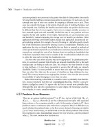
bol depends only on the previous symbol. Figure 8.9 is an example Markov chain model.
A Markov chain model is defined by (a) a set of states, Q, which emit symbols and (b) a
set of transitions between states. States are represented by circles and transitions are rep-
resented by arrows. Each transition has an associated transition probability, a
i j
, which
represents the conditional probability of going to state j in the next step, given that the
current state is i. The sum of all transition probabilities from a given state must equal 1,
that is,
∑
j∈Q

a
i j
= 1 for all j ∈ Q. If an arc is not shown, it is assumed to have a 0 prob-
ability. The transition probabilities can also be written as a transition matrix, A = {a
i j
}.
Example 8.16
Markov chain. The Markov chain in Figure 8.9 is a probabilistic model for CpG islands.
The states are A, C, G, and T. For readability, only some of the transition probabilities
are shown. For example, the transition probability from state G to state T is 0.14, that is,
P(x
i
= T|x
i−1
= G) = 0.14. Here, the emitted symbols are understood. For example, the
symbol C is emitted when transitioning from state C. In speech recognition, the symbols
emitted could represent spoken words or phrases.
Given some sequence x of length L, how probable is x given the model? If x is a DNA
sequence, we could use our Markov chain model to determine how probable it is that x
is from a CpG island. To do so, we look at the probability of x as a path, x
1
x
2
x
L
, in
the chain. This is the probability of starting in the first state, x
1
, and making successive
transitions to x

2
, x
3
, and so on, to x
L
. In a Markov chain model, the probability of x
L
A G
TC
0.14
0.44
0.36
Figure 8.9 A Markov chain model.
520 Chapter 8 Mining Stream, Time-Series, and Sequence Data
depends on the value of only the previous one state, x
L−1
, not on the entire previous
sequence.
9
This characteristic is known as the Markov property, which can be written as
P(x) = P(x
L
|x
L−1
)P(x
L−1
|x
L−2
)···P(x
2

|x
1
)P(x
1
)
(8.7)
= P(x
1
)
L
∏
i=2
P(x
i
|x
i−1
).
That is, the Markov chain can only “remember” the previous one state of its history.
Beyond that, it is “memoryless.”
In Equation (8.7), we need to specify P(x
1
), the probability of the starting state. For
simplicity, we would like to model this as a transition too. This can be done by adding
a begin state, denoted 0, so that the starting state becomes x
0
= 0. Similarly, we can add
an end state, also denoted as 0. Note that P(x
i
|x
i−1

) is the transition probability, a
x
i−1
x
i
.
Therefore, Equation (8.7) can be rewritten as
P(x) =
L
∏
i=1
a
x
i−1
x
i
, (8.8)
which computesthe probability that sequence xbelongs to the given Markov chain model,
that is, P(x|model). Note that the begin and end states are silent in that they do not emit
symbols in the path through the chain.
We can use the Markov chain model for classification. Suppose that we want to distin-
guish CpG islands from other “non-CpG” sequence regions. Given training sequences
from CpG islands (labeled “+”) and from non-CpG islands (labeled “−”), we can con-
struct two Markov chain models—the first, denoted “+”, to represent CpG islands, and
the second, denoted “−”, to represent non-CpG islands. Given a sequence, x, we use the
respective models to compute P(x|+), the probability that x is from a CpG island, and
P(x|−), the probability that it is from a non-CpG island. The log-odds ratio can then be
used to classify x based on these two probabilities.
“But first, how can we estimate the transition probabilities for each model?” Before we
can compute the probability of xbeing from either of the two models, we need to estimate

the transition probabilities for the models. Given the CpG (+) training sequences, we can
estimate the transition probabilities for the CpG island model as
a
+
i j
=
c
+
i j
∑
k
c
+
ik
, (8.9)
where c
+
i j
is the number of times that nucleotide j follows nucleotide i in the given
sequences labeled “+”. For the non-CpG model, we use the non-CpG island sequences
(labeled “−”) in a similar way to estimate a
−
i j
.
9
This is known as a first-order Markov chain model, since x
L
depends only on the previous state, x
L−1
.

In general, for the k-th-order Markov chain model, the probability of x
L
depends on the values of only
the previous k states.
8.4 Mining Sequence Patterns in Biological Data 521
To determine whether x is from a CpG island or not, we compare the models using
the logs-odds ratio, defined as
log
P(x|+)
P(x|−)
=
L
∑
i=1
log
a
+
x
i−1
x
i
a
−
x
i−1
x
i
. (8.10)
If this ratio is greater than 0, then we say that x is from a CpG island.
Example 8.17

Classification using a Markov chain. Our model for CpG islands and our model for
non-CpG islands both have the same structure, as shown in our example Markov chain
of Figure 8.9. Let CpG
+
be the transition matrix for the CpG island model. Similarly,
CpG
−
is the transition matrix for the non-CpG island model. These are (adapted from
Durbin, Eddy, Krogh, and Mitchison [DEKM98]):
CpG
+
=








A C G T
A 0.20 0.26 0.44 0.10
C 0.16 0.36 0.28 0.20
G 0.15 0.35 0.36 0.14
T 0.09 0.37 0.36 0.18









(8.11)
CpG
−
=








A C G T
A 0.27 0.19 0.31 0.23
C 0.33 0.31 0.08 0.28
G 0.26 0.24 0.31 0.19
T 0.19 0.25 0.28 0.28








(8.12)
Notice that the transition probability a

+
CG
= 0.28 is higher than a
−
CG
= 0.08. Suppose we
are given the sequence x = CGCG. The log-odds ratio of x is
log
0.28
0.08
+ log
0.35
0.24
+ log
0.28
0.08
= 1.25 > 0.
Thus, we say that x is from a CpG island.
In summary, we can use a Markov chain model to determine if a DNA sequence, x, is
from a CpG island. This was the first of our two important questions mentioned at the
beginning of this section. To answer the second question, that of finding all of the CpG
islands in a given sequence, we move on to hidden Markov models.
Hidden Markov Model
Given a long DNA sequence, how can we find all CpG islands within it? We could try
the Markov chain method above, using a sliding window. For each window, we could
522 Chapter 8 Mining Stream, Time-Series, and Sequence Data
compute the log-odds ratio. CpG islands within intersecting windows could be merged
to determine CpG islands within the long sequence. This approach has some difficulties:
It is not clear what window size to use, and CpG islands tend to vary in length.
What if, instead, we merge the two Markov chains from above (for CpG islands and

non-CpG islands, respectively) and add transition probabilities between the two chains?
The result is a hidden Markov model, as shown in Figure 8.10. The states are renamed
by adding “+” and “−” labels to distinguish them. For readability, only the transitions
between “+” and “−” states are shown, in addition to those for the begin and end states.
Let π = π
1
π
2
π
L
be a path of states that generates a sequence of symbols, x = x
1
x
2
x
L
.
In a Markov chain, the path through the chain for x is unique. With a hidden Markov
model, however, different paths can generate the same sequence. For example, the states
C
+
and C
−
both emit the symbol C. Therefore, we say the model is “hidden” in that
we do not know for sure which states were visited in generating the sequence. The tran-
sition probabilities between the original two models can be determined using training
sequences containing transitions between CpG islands and non-CpG islands.
A Hidden Markov Model (HMM) is defined by
a set of states, Q
a set of transitions, where transition probability a

kl
= P(π
i
= l|π
i−1
= k) is the prob-
ability of transitioning from state k to state l for k, l ∈ Q
an emission probability, e
k
(b) = P(x
i
= b|π
i
= k), for each state, k, and each symbol,
b, where e
k
(b) is the probability of seeing symbol b in state k. The sum of all emission
probabilities at a given state must equal 1, that is,
∑
b
e
k
= 1 for each state, k.
Example 8.18
A hidden Markov model. The transition matrix for the hidden Markov model of
Figure 8.10 is larger than that of Example 8.16 for our earlier Markov chain example.
G
+
C
+

G
–
C
–
T
+
A
+
T
–
A
–
O O
Figure 8.10 A hidden Markov model.
8.4 Mining Sequence Patterns in Biological Data 523
It contains the states A
+
, C
+
, G
+
, T
+
, A
−
, C
−
, G
−
, T

−
(not shown). The transition
probabilities between the “+” states are as before. Similarly, the transition probabili-
ties between the “−” states are as before. The transition probabilities between “+” and
“−” states can be determined as mentioned above, using training sequences containing
known transitions from CpG islands to non-CpG islands, and vice versa. The emis-
sion probabilities are e
A
+
(A) = 1, e
A
+
(C) = 0, e
A
+
(G) = 0, e
A
+
(T) = 0, e
A
−
(A) = 1,
e
A
−
(C) = 0, e
A
−
(G) = 0, e
A

−
(T) = 0, and so on. Although here the probability of emit-
ting a symbol at a state is either 0 or 1, in general, emission probabilities need not be
zero-one.
Tasks using hidden Markov models include:
Evaluation: Given a sequence, x, determine the probability, P(x), of obtaining x in the
model.
Decoding: Given a sequence, determine the most probable path through the model
that produced the sequence.
Learning: Given a model and a set of training sequences, find the model parameters
(i.e., the transition and emission probabilities) that explain the training sequences
with relatively high probability. The goal is to find a model that generalizes well to
sequences we have not seen before.
Evaluation, decoding, and learning can be handled using the forward algorithm,
Viterbi algorithm, and Baum-Welch algorithm, respectively. These algorithms are dis-
cussed in the following sections.
Forward Algorithm
What is the probability, P(x), that sequence x was generated by a given hidden Markov
model (where, say, the model represents a sequence class)? This problem can be solved
using the forward algorithm.
Let x = x
1
x
2
x
L
be our sequence of symbols. A path is a sequence of states. Many
paths can generate x. Consider one such path, which we denote π = π
1
π

2
π
L
. If we
incorporate the begin and end states, denoted as 0, we can write π as π
0
= 0, π
1
π
2
π
L
,
π
L+1
= 0. The probability that the model generated sequence x using path π is
P(x, π) = a
0π
1
e
π
1
(x
1
) ·a
π
1
π
2
e

π
2
(x
2
) ····a
π
L−1
π
L
e
π
L
(x
L
) ·a
π
L
0
(8.13)
= a
0π
1
L
∏
i=1
e
π
i
(x
i

)a
π
i
π
i+1
where π
L+1
= 0. We must, however, consider all of the paths that can generate x. There-
fore, the probability of x given the model is
P(x) =
∑
π
P(x, π). (8.14)
That is, we add the probabilities of all possible paths for x.
524 Chapter 8 Mining Stream, Time-Series, and Sequence Data
Algorithm: Forward algorithm. Find the probability, P(x), that sequence x was generated by the given hidden
Markov model.
Input:
A hidden Markov model, defined by a set of states, Q, that emit symbols, and by transition and emission
probabilities;
x, a sequence of symbols.
Output: Probability, P(x).
Method:
(1) Initialization (i = 0): f
0
(0) = 1, f
k
(0) = 0 for k > 0
(2) Recursion (i = 1 L): f
l

(i) = e
l
(x
i
)
∑
k
f
k
(i−1)a
kl
(3) Termination: P(x) =
∑
k
f
k
(L)a
k0
Figure 8.11 Forward algorithm.
Unfortunately, the number of paths can be exponential with respect to the length,
L, of x, so brute force evaluation by enumerating all paths is impractical. The forward
algorithm exploits a dynamic programming technique to solve this problem. It defines
forward variables, f
k
(i), to be the probability of being in state k having observed the first
i symbols of sequence x. We want to compute f
π
L+1=0
(L), the probability of being in the
end state having observed all of sequence x.

The forward algorithm is shown in Figure 8.11. It consists of three steps. In step 1,
the forward variables are initialized for all states. Because we have not viewed any part of
the sequence at this point, the probability of being in the start state is 1 (i.e., f
0
(0) = 1),
and the probability of being in any other state is 0. In step 2, the algorithm sums over all
the probabilities of all the paths leading from one state emission to another. It does this
recursively for each move from state to state. Step 3 gives the termination condition. The
whole sequence (of length L) has been viewed, and we enter the end state, 0. We end up
with the summed-over probability of generating the required sequence of symbols.
Viterbi Algorithm
Given a sequence, x, what is the most probable path in the model that generates x? This
problem of decoding can be solved using the Viterbi algorithm.
Many paths can generate x. We want to find the most probable one, π

, that is, the
path that maximizes the probability of having generated x. This is π

= argmax
π
P(π|x).
10
It so happens that this is equal to argmax
π
P(x, π). (The proof is left as an exercise for the
reader.) We saw how to compute P(x, π) in Equation (8.13). For a sequence of length L,
there are |Q|
L
possible paths, where |Q| is the number of states in the model. It is
10

In mathematics, argmax stands for the argument of the maximum. Here, this means that we want the
path, π, for which P(π|x) attains its maximum value.
8.4 Mining Sequence Patterns in Biological Data 525
infeasible to enumerate all of these possible paths! Once again, we resort to a dynamic
programming technique to solve the problem.
At each step along the way, the Viterbi algorithm tries to find the most probable
path leading from one symbol of the sequence to the next. We define v
l
(i) to be the
probability of the most probable path accounting for the first i symbols of x and
ending in state l. To find π

, we need to compute max
k
v
k
(L), the probability of the
most probable path accounting for all of the sequence and ending in the end state.
The probability, v
l
(i), is
v
l
(i) = e
l
(x
i
) ·max
k
(v

l
(k)a
kl
), (8.15)
which states that the most probable path that generates x
1
x
i
and ends in state l has to
emit x
i
in state x
l
(hence, the emission probability, e
l
(x
i
)) and has to contain the most
probable path that generates x
1
x
i−1
and ends in state k, followed by a transition from
state k to state l (hence, the transition probability, a
kl
). Thus, we can compute v
k
(L) for
any state, k, recursively to obtain the probability of the most probable path.
The Viterbi algorithm is shown in Figure 8.12. Step 1 performs initialization. Every

path starts at the begin state (0) with probability 1. Thus, for i = 0, we have v
0
(0) = 1, and
the probability of starting at any other state is 0. Step 2 applies the recurrence formula for
i = 1 to L. At each iteration, we assume that we know the most likely path for x
1
x
i−1
that ends in state k, for all k ∈Q. To find the most likely path to the i-th state from there,
we maximize v
k
(i−1)a
kl
over all predecessors k ∈Q of l. To obtain v
l
(i), we multiply by
e
l
(x
i
) since we have to emit x
i
from l. This gives us the first formula in step 2. The values
v
k
(i) are stored in a Q×L dynamic programming matrix. We keep pointers (ptr) in this
matrix so that we can obtain the path itself. The algorithm terminates in step 3, where
finally, we have max
k
v

k
(L). We enter the end state of 0 (hence, the transition probability,
a
k0
) but do not emit a symbol. The Viterbi algorithm runs in O(|Q|
2
|L|) time. It is more
efficient than the forward algorithm because it investigates only the most probable path
and avoids summing over all possible paths.
Algorithm: Viterbi algorithm. Find the most probable path that emits the sequence of symbols, x.
Input:
A hidden Markov model, defined by a set of states, Q, that emit symbols, and by transition and emission
probabilities;
x, a sequence of symbols.
Output: The most probable path, π
∗
.
Method:
(1) Initialization (i = 0): v
0
(0) = 1, v
k
(0) = 0 for k > 0
(2) Recursion (i = 1 L): v
l
(i) = e
l
(x
i
)max

k
(v
k
(i−1)a
kl
)
ptr
i
(l) = argmax
k
(v
k
(i−1)a
kl
)
(3) Termination: P(x,π
∗
) = max
k
(v
k
(L)a
k0
)
π
∗
L
= argmax
k
(v

k
(L)a
k0
)
Figure 8.12 Viterbi (decoding) algorithm.
526 Chapter 8 Mining Stream, Time-Series, and Sequence Data
Baum-Welch Algorithm
Given a training set of sequences, how can we determine the parameters of a hidden
Markov model that will best explain the sequences? In other words, we want to learn or
adjust the transition and emission probabilities of the model so that it can predict the
path of future sequences of symbols. If we know the state path for each training sequence,
learning the model parameters is simple. We can compute the percentage of times each
particular transition or emission is used in the set of training sequences to determine a
kl
,
the transition probabilities, and e
k
(b), the emission probabilities.
When the paths for the training sequences are unknown, there is no longer a direct
closed-form equation for the estimated parameter values. An iterative procedure must be
used, like the Baum-Welch algorithm. The Baum-Welch algorithm is a special case of the
EM algorithm (Section 7.8.1), which is a family of algorithms for learning probabilistic
models in problems that involve hidden states.
The Baum-Welch algorithm is shown in Figure 8.13. The problem of finding the
optimal transition and emission probabilities is intractable. Instead, the Baum-Welch
algorithm finds a locally optimal solution. In step 1, it initializes the probabilities to
an arbitrary estimate. It then continuously re-estimates the probabilities (step 2) until
convergence (i.e., when there is very little change in the probability values between iter-
ations). The re-estimation first calculates the expected transmission and emission prob-
abilities. The transition and emission probabilities are then updated to maximize the

likelihood of the expected values.
In summary, Markov chains and hidden Markov models are probabilistic models in
which the probability of a state depends only on that of the previous state. They are par-
ticularly useful for the analysis of biological sequence data, whose tasks include evalua-
tion, decoding, and learning. We have studied the forward, Viterbi, and Baum-Welch
algorithms. The algorithms require multiplying many probabilities, resulting in very
Algorithm: Baum-Welch algorithm. Find the model parameters (transition and emission probabilities) that
best explain the training set of sequences.
Input:
A training set of sequences.
Output:
Transition probabilities, a
kl
;
Emission probabilities, e
k
(b);
Method:
(1) initialize the transmission and emission probabilities;
(2) iterate until convergence
(2.1) calculate the expected number of times each transition or emission is used
(2.2) adjust the parameters to maximize the likelihood of these expected values
Figure 8.13 Baum-Welch (learning) algorithm.
8.5 Summary 527
small numbers that can cause underflow arithmetic errors. A way around this is to use
the logarithms of the probabilities.
8.5
Summary
Stream data flow in and out of a computer system continuously and with varying
update rates. They are temporally ordered, fast changing, massive (e.g., gigabytes to ter-

abytes in volume), and potentially infinite. Applications involving stream data include
telecommunications, financial markets, and satellite data processing.
Synopses provide summaries of stream data, which typically can be used to return
approximate answers to queries. Random sampling, slidingwindows,histograms, mul-
tiresolution methods (e.g., for data reduction), sketches (which operate in a single
pass), and randomized algorithms are all forms of synopses.
The tilted time frame model allows data to be stored at multiple granularities of time.
The most recent time is registered at the finest granularity. The most distant time is
at the coarsest granularity.
A stream data cube can store compressed data by (1) using thetilted time frame model
on the time dimension, (2) storing data at only some critical layers, which reflect
the levels of data that are of most interest to the analyst, and (3) performing partial
materialization based on “popular paths” through the critical layers.
Traditional methods of frequent itemset mining, classification, and clustering tend to
scan the data multiple times, making them infeasible for stream data. Stream-based
versionsofsuchmininginsteadtry tofindapproximateanswerswithinauser-specified
error bound. Examples include the Lossy Counting algorithm for frequent itemset
stream mining; the Hoeffding tree, VFDT, and CVFDT algorithms for stream data
classification; and the STREAM and CluStream algorithms for stream data clustering.
A time-series database consists of sequences of values or events changing with time,
typically measured at equal time intervals. Applications include stock market analysis,
economic and sales forecasting, cardiogram analysis, and the observation of weather
phenomena.
Trend analysis decomposes time-series data into the following: trend (long-term)
movements, cyclic movements, seasonal movements (which are systematic or calendar
related), and irregular movements (due to random or chance events).
Subsequence matching is a form of similarity search that finds subsequences that
are similar to a given query sequence. Such methods match subsequences that have
the same shape, while accounting for gaps (missing values) and differences in base-
line/offset and scale.

A sequence database consists of sequences of ordered elements or events, recorded
with or without a concrete notion of time. Examples of sequence data include cus-
tomer shopping sequences, Web clickstreams, and biological sequences.
528 Chapter 8 Mining Stream, Time-Series, and Sequence Data
Sequential pattern mining is the mining of frequently occurring ordered events or
subsequences as patterns. Given a sequence database, any sequence that satisfies min-
imum support is frequent and is called a sequential pattern. An example of a sequen-
tial pattern is “Customers who buy a Canon digital camera are likely to buy an HP
color printer within a month.” Algorithms for sequential pattern mining include GSP,
SPADE, and PrefixSpan, as well as CloSpan (which mines closed sequential patterns).
Constraint-based mining of sequential patterns incorporates user-specified
constraints to reduce the search space and derive only patterns that are of interest
to the user. Constraints may relate to the duration of a sequence, to an event fold-
ing window (where events occurring within such a window of time can be viewed as
occurring together), and to gaps between events. Pattern templates may also be spec-
ified as a form of constraint using regular expressions.
Periodicity analysis is the mining of periodic patterns, that is, the search for recurring
patterns in time-related sequence databases. Full periodic and partial periodic patterns
can be mined, as well as periodic association rules.
Biological sequence analysis compares, aligns, indexes, and analyzes biological
sequences, which can be either sequences of nucleotides or of amino acids. Biose-
quenceanalysisplaysacrucialroleinbioinformaticsandmodernbiology.Suchanalysis
can be partitioned into two essential tasks: pairwise sequence alignment and multi-
ple sequence alignment. The dynamic programming approach is commonly used for
sequence alignments. Among many available analysis packages, BLAST (Basic Local
Alignment Search Tool) is one of the most popular tools in biosequence analysis.
Markov chains and hidden Markov models are probabilistic models in which the
probability of a state depends only on that of the previous state. They are particu-
larly useful for the analysis of biological sequence data. Given a sequence of symbols,
x, the forward algorithm finds the probability of obtaining x in the model, whereas

the Viterbi algorithm finds the most probable path (corresponding to x) through the
model. The Baum-Welch algorithm learns or adjusts the model parameters (transition
and emission probabilities) so as to best explain a set of training sequences.
Exercises
8.1 A stream data cube should be relatively stable in size with respect to infinite data streams.
Moreover, it should be incrementally updateable with respect to infinite data streams.
Show that the stream cube proposed in Section 8.1.2 satisfies these two requirements.
8.2 In stream data analysis, we are often interested in only the nontrivial or exceptionally
large cube cells. These can be formulated as iceberg conditions. Thus, it may seem that
the iceberg cube [BR99] is a likely model for stream cube architecture. Unfortunately,
this is not the case because iceberg cubes cannot accommodate the incremental updates
required due to the constant arrival of new data. Explain why.
Exercises 529
8.3 An important task in stream data analysis is to detect outliers in a multidimensional
environment. An example is the detection of unusual power surges, where the dimen-
sions include time (i.e., comparing with the normal duration), region (i.e., comparing
with surrounding regions), sector (i.e., university, residence, government), and so on.
Outline an efficient stream OLAP method that can detect outliers in data streams. Pro-
vide reasons as to why your design can ensure such quality.
8.4 Frequent itemset mining in data streams is a challenging task. It is too costly to keep the
frequency count for every itemset. However, because a currently infrequent itemset may
become frequent, and a currently frequent one may become infrequent in the future,
it is important to keep as much frequency count information as possible. Given a fixed
amount of memory,can you work out a good mechanism that may maintain high-quality
approximation of itemset counting?
8.5 For the above approximate frequent itemset counting problem, it is interesting to incor-
porate the notion of tilted time frame. That is, we can put less weight on more remote
itemsets when counting frequent itemsets. Design an efficient method that may obtain
high-quality approximation of itemset frequency in data streams in this case.
8.6 A classification model may change dynamically along with the changes of training data

streams. This is known as concept drift. Explain why decision tree induction may not
be a suitable method for such dynamically changing data sets. Is naïve Bayesian a better
method on such data sets? Comparing with the naïve Bayesian approach, is lazy evalua-
tion (such as the k-nearest-neighbor approach) even better? Explain your reasoning.
8.7 The concept of microclustering has been popular for on-line maintenance of cluster-
ing information for data streams. By exploring the power of microclustering, design an
effective density-based clustering method for clustering evolving data streams.
8.8 Suppose that a power station stores data regarding power consumption levels by time and
by region, in addition to power usage information per customer in each region. Discuss
how to solve the following problems in such a time-series database:
(a) Find similar power consumption curve fragments for a given region on Fridays.
(b) Every time a power consumption curve rises sharply, what may happen within the
next 20 minutes?
(c) How can we find the most influential features that distinguish a stable power con-
sumption region from an unstable one?
8.9 Regression is commonly used in trend analysis for time-series data sets. An item in a
time-series database is usually associated with properties in multidimensional space.
For example, an electric power consumer may be associated with consumer location,
category, and time of usage (weekdays vs. weekends). In such a multidimensional
space, it is often necessary to perform regression analysis in an OLAP manner (i.e.,
drilling and rolling along any dimension combinations that a user desires). Design
an efficient mechanism so that regression analysis can be performed efficiently in
multidimensional space.
530 Chapter 8 Mining Stream, Time-Series, and Sequence Data
8.10 Suppose that a restaurant chain would like to mine customers’ consumption behavior
relating to major sport events, such as “Every time there is a major sport event on TV, the
sales of Kentucky Fried Chicken will go up 20% one hour before the match.”
(a) For this problem, there are multiple sequences (each corresponding to one restau-
rant in the chain). However, each sequence is long and contains multiple occurrences
of a (sequential) pattern. Thus this problem is different from the setting of sequential

pattern mining problem discussed in this chapter. Analyze what are the differences
in the two problem definitions and how such differences may influence the develop-
ment of mining algorithms.
(b) Develop a method for finding such patterns efficiently.
8.11 (Implementation project) The sequential pattern mining algorithm introduced by
Srikant and Agrawal [SA96] finds sequential patterns among a set of sequences. Although
there have been interesting follow-up studies, such as the development of the algorithms
SPADE (Zaki [Zak01]), PrefixSpan (Pei, Han, Mortazavi-Asl, et al. [PHMA
+
01]), and
CloSpan (Yan, Han, and Afshar [YHA03]), the basic definition of “sequential pattern”
has not changed. However, suppose we would like to find frequently occurring subse-
quences (i.e., sequential patterns) within one given sequence, where, say, gaps are not
allowed. (That is, we do not consider AG to be a subsequence of the sequence ATG.)
For example, the string ATGCTCGAGCT contains a substring GCT with a support of
2. Derive an efficient algorithm that finds the complete set of subsequences satisfying a
minimum support threshold. Explain how your algorithm works using a small example,
and show some performance results for your implementation.
8.12 Suppose frequent subsequences have been mined from a sequence database, with a given
(relative) minimum support, min
sup. The database can be updated in two cases:
(i) adding new sequences (e.g., new customers buying items), and (ii) appending new
subsequences to some existing sequences (e.g., existing customers buying new items). For
each case, work out an efficient incremental mining method that derives the complete sub-
sequences satisfying min
sup, without mining the whole sequence database from scratch.
8.13 Closed sequential patterns can be viewed as a lossless compression of a large set of sequen-
tial patterns. However, the set of closed sequential patterns may still be too large for effec-
tive analysis. There should be some mechanism for lossy compression that may further
reduce the set of sequential patterns derived from a sequence database.

(a) Provide a good definition of lossy compression of sequential patterns, and reason
why such a definition may lead to effective compression with minimal information
loss (i.e., high compression quality).
(b) Develop an efficient method for such pattern compression.
(c) Develop an efficient method that mines such compressed patterns directly from a
sequence database.
8.14 As discussed in Section 8.3.4, mining partial periodic patterns will require a user to spec-
ify the length of the period. This may burden the user and reduces the effectiveness of
Bibliographic Notes 531
mining. Propose a method that will automatically mine the minimal period of a pattern
without requiring a predefined period. Moreover, extend the method to find approximate
periodicity where the period will not need to be precise (i.e., it can fluctuate within a
specified small range).
8.15 There are several major differences between biological sequential patterns and transac-
tional sequential patterns. First, in transactional sequential patterns, the gaps between
two events are usually nonessential. For example, the pattern “purchasing a digital camera
two months after purchasing a PC” does not imply that the two purchases are consecutive.
However, for biological sequences, gaps play an important role in patterns. Second, pat-
terns in a transactional sequence are usually precise. However, a biological pattern can be
quite imprecise, allowing insertions, deletions, and mutations. Discuss how the mining
methodologies in these two domains are influenced by such differences.
8.16 BLAST is a typical heuristic alignment method for pairwise sequence alignment. It first
locates high-scoring short stretches and then extends them to achieve suboptimal align-
ments. When the sequences to be aligned are really long, BLAST may run quite slowly.
Propose and discuss some enhancements to improve the scalability of such a method.
8.17 The Viterbi algorithm uses the equality, argmax
π
P(π|x) = argmax
π
P(x, π), in its search

for the most probable path, π
∗
, through a hidden Markov model for a given sequence of
symbols, x. Prove the equality.
8.18 (Implementation project) A dishonest casino uses a fair die most of the time. However, it
switches to a loaded die with a probability of 0.05, and switches back to the fair die with
a probability 0.10. The fair die has a probability of
1
6
of rolling any number. The loaded
die has P(1) = P(2) = P(3) = P(4) = P(5) = 0.10 and P(6) = 0.50.
(a) Draw a hidden Markov model for the dishonest casino problem using two states,
Fair (F) and Loaded (L). Show all transition and emission probabilities.
(b) Suppose you pick up a die at random and roll a 6. What is the probability that the
die is loaded, that is, find P(6|D
L
)? What is the probability that it is fair, that is, find
P(6|D
F
)? What is the probability of rolling a 6 from the die you picked up? If you
roll a sequence of 666, what is the probability that the die is loaded?
(c) Write a program that, given a sequence of rolls (e.g., x = 5114362366. ), predicts
when the fair die was used and when the loaded die was used. (Hint: This is similar
to detecting CpG islands and non-CPG islands in a given long sequence.) Use the
Viterbi algorithm to get the most probable path through the model. Describe your
implementation in report form, showing your code and some examples.
Bibliographic Notes
Stream data mining research has been active in recent years. Popular surveys on stream
data systems and stream data processing include Babu and Widom [BW01], Babcock,
Babu, Datar, et al. [BBD

+
02], Muthukrishnan [Mut03], and the tutorial by Garofalakis,
Gehrke, and Rastogi [GGR02].
532 Chapter 8 Mining Stream, Time-Series, and Sequence Data
There have been extensive studies on stream data management and the processing
of continuous queries in stream data. For a description of synopsis data structures for
stream data, see Gibbons and Matias [GM98]. Vitter introduced the notion of reservoir
sampling as a way to select an unbiased random sample of n elements without replace-
ment from a larger ordered set of size N, where N is unknown [Vit85]. Stream query
or aggregate processing methods have been proposed by Chandrasekaran and Franklin
[CF02], Gehrke, Korn, and Srivastava [GKS01], Dobra, Garofalakis, Gehrke, and Ras-
togi [DGGR02], and Madden, Shah, Hellerstein, and Raman [MSHR02]. A one-pass
summary method for processing approximate aggregate queries using wavelets was pro-
posed by Gilbert, Kotidis, Muthukrishnan, and Strauss [GKMS01]. Statstream, a statisti-
cal method for the monitoring of thousands of data streams in real time, was developed
by Zhu and Shasha [ZS02, SZ04].
There are also many stream data projects. Examples include Aurora by Zdonik,
Cetintemel, Cherniack, et al. [ZCC
+
02], which is targeted toward stream monitoring
applications; STREAM, developed at Stanford University by Babcock, Babu, Datar,
et al., aims at developing a general-purpose Data Stream Management System (DSMS)
[BBD
+
02]; and an early system called Tapestry by Terry, Goldberg, Nichols, and Oki
[TGNO92], which used continuous queries for content-based filtering over an append-
only database of email and bulletin board messages. A restricted subset of SQL was
used as the query language in order to provide guarantees about efficient evaluation
and append-only query results.
A multidimensional stream cube model was proposed by Chen, Dong, Han, et al.

[CDH
+
02] in their study of multidimensional regression analysis of time-series data
streams. MAIDS (Mining Alarming Incidents from Data Streams), a stream data mining
system built on top of such a stream data cube, was developed by Cai, Clutter, Pape, et al.
[CCP
+
04].
For mining frequent items and itemsets on stream data, Manku and Motwani pro-
posed sticky sampling and lossy counting algorithms for approximate frequency counts
over data streams [MM02]. Karp, Papadimitriou, and Shenker proposed a counting algo-
rithm for finding frequent elements in data streams [KPS03]. Giannella, Han, Pei, et al.
proposed a method for mining frequent patterns in data streams at multiple time gran-
ularities [GHP
+
04]. Metwally, Agrawal, and El Abbadi proposed a memory-efficient
method for computing frequent and top-k elements in data streams [MAA05].
For stream data classification, Domingos and Hulten proposed the VFDT algorithm,
based on their Hoeffding tree algorithm [DH00]. CVFDT, a later version of VFDT, was
developed by Hulten, Spencer, and Domingos [HSD01] to handle concept drift in time-
changing data streams. Wang, Fan, Yu, and Han proposed an ensemble classifier to mine
concept-drifting data streams [WFYH03]. Aggarwal, Han, Wang, and Yu developed a
k-nearest-neighbor-based method for classify evolving data streams [AHWY04b].
Several methods have been proposed for clustering data streams. The k-median-
based STREAM algorithm was proposed by Guha, Mishra, Motwani, and O’Callaghan
[GMMO00] and by O’Callaghan, Mishra, Meyerson, et al. [OMM
+
02]. Aggarwal, Han,
Wang, and Yu proposed CluStream, a framework for clustering evolving data streams
Bibliographic Notes 533

[AHWY03], and HPStream, a framework for projected clustering of high-dimensional
data streams [AHWY04a].
Statistical methods fortime-series analysishavebeen proposedandstudied extensively
in statistics, suchasinChatfield [Cha03], Brockwell and Davis [BD02],andShumway and
Stoffer[SS05].StatSoft’s ElectronicTextbook(www.statsoft.com/textbook/stathome.html)
is a useful online resource that includes a discussion on time-series data analysis. The
ARIMA forecasting method is described in Box, Jenkins, and Reinsel [BJR94]. Efficient
similarity search in sequence databases was studied by Agrawal, Faloutsos, and Swami
[AFS93]. A fast subsequence matching method in time-series databases was presented by
Faloutsos, Ranganathan, and Manolopoulos [FRM94]. Agrawal, Lin, Sawhney, and Shim
[ALSS95] developed a method for fast similarity search in the presence of noise, scaling,
and translation in time-series databases. Language primitives for querying shapes of his-
tories were proposed by Agrawal, Psaila, Wimmers, and Zait [APWZ95]. Other work on
similarity-based search of time-series data includes Rafiei and Mendelzon [RM97], and
Yi, Jagadish, and Faloutsos [YJF98]. Yi, Sidiropoulos, Johnson, Jagadish, et al. [YSJ
+
00]
introduced a method for on-line mining for co-evolving time sequences. Chen, Dong,
Han, et al. [CDH
+
02] proposed a multidimensional regression method for analysis of
multidimensional time-series data. Shasha and Zhu present a state-of-the-art overview of
the methods for high-performance discovery in time series [SZ04].
The problem of mining sequential patterns was first proposed by Agrawal and Srikant
[AS95]. In the Apriori-based GSP algorithm, Srikant and Agrawal [SA96] generalized
their earlier notion to include time constraints, a sliding time window, and user-defined
taxonomies. Zaki [Zak01] developed a vertical-format-based sequential pattern mining
method called SPADE, which is an extension of vertical-format-based frequent itemset
mining methods, like Eclat and Charm [Zak98, ZH02]. PrefixSpan, a pattern growth
approach to sequential pattern mining, and its predecessor, FreeSpan, were developed

by Pei, Han, Mortazavi-Asl, et al. [HPMA
+
00, PHMA
+
01, PHMA
+
04]. The CloSpan
algorithm for mining closed sequential patterns was proposed by Yan, Han, and Afshar
[YHA03]. BIDE, a bidirectional search for mining frequent closed sequences, was devel-
oped by Wang and Han [WH04].
The studies of sequential pattern mining have been extended in several different
ways. Mannila, Toivonen, and Verkamo [MTV97] consider frequent episodes in se-
quences, where episodes are essentially acyclic graphs of events whose edges specify
the temporal before-and-after relationship but without timing-interval restrictions.
Sequence pattern mining for plan failures was proposed in Zaki, Lesh, and Ogihara
[ZLO98]. Garofalakis, Rastogi, and Shim [GRS99a] proposed the use of regular expres-
sions as a flexible constraint specification tool that enables user-controlled focus to be
incorporated into the sequential pattern mining process. The embedding of multidi-
mensional, multilevel information into a transformed sequence database for sequen-
tial pattern mining was proposed by Pinto, Han, Pei, et al. [PHP
+
01]. Pei, Han, and
Wang studied issues regarding constraint-based sequential pattern mining [PHW02].
CLUSEQ is a sequence clustering algorithm, developed by Yang and Wang [YW03].
An incremental sequential pattern mining algorithm, IncSpan, was proposed by
Cheng, Yan, and Han [CYH04]. SeqIndex, efficient sequence indexing by frequent and
534 Chapter 8 Mining Stream, Time-Series, and Sequence Data
discriminative analysis of sequential patterns, was studied by Cheng, Yan, and Han
[CYH05]. A method for parallel mining of closed sequential patterns was proposed
by Cong, Han, and Padua [CHP05].

Data mining for periodicity analysis has been an interesting theme in data mining.
Özden, Ramaswamy, and Silberschatz [ORS98] studied methods for mining periodic
or cyclic association rules. Lu, Han, and Feng [LHF98] proposed intertransaction asso-
ciation rules, which are implication rules whose two sides are totally ordered episodes
with timing-interval restrictions (on the events in the episodes and on the two sides).
Bettini, Wang, and Jajodia [BWJ98] consider a generalization of intertransaction associ-
ation rules. The notion of mining partial periodicity was first proposed by Han, Dong,
and Yin, together with a max-subpattern hit set method [HDY99]. Ma and Hellerstein
[MH01a] proposed a method for mining partially periodic event patterns with unknown
periods. Yang, Wang, and Yu studied mining asynchronous periodic patterns in time-
series data [YWY03].
Methods for the analysis of biological sequences have been introduced in many text-
books, such as Waterman [Wat95], Setubal and Meidanis [SM97], Durbin, Eddy, Krogh,
and Mitchison [DEKM98], Baldi and Brunak [BB01], Krane and Raymer [KR03], Jones
and Pevzner [JP04], and Baxevanis and Ouellette [BO04]. BLAST was developed by
Altschul, Gish, Miller, et al. [AGM
+
90]. Information about BLAST can be found
at the NCBI Web site www.ncbi.nlm.nih.gov/BLAST/. For a systematic introduction of
the BLAST algorithms and usages, see the book “BLAST” by Korf, Yandell, and
Bedell [KYB03].
For an introduction to Markov chains and hidden Markov models from a biological
sequence perspective, see Durbin, Eddy, Krogh, and Mitchison [DEKM98] and Jones and
Pevzner [JP04]. A generalintroduction can be found inRabiner [Rab89]. EddyandKrogh
have each respectively headed the development of software packages for hidden Markov
modelsforproteinsequenceanalysis,namelyHMMER(pronounced“hammer,”available
at and SAM (www.cse.ucsc.edu/research/ compbio/sam.html).
9
Graph Mining, Social Network
Analysis, and Multirelational

Data Mining
We have studied frequent-itemset mining in Chapter 5 and sequential-pattern mining in Section
3 of Chapter 8. Many scientific and commercial applications need patterns that are more
complicated than frequent itemsets and sequential patterns and require extra effort to
discover. Such sophisticated patterns go beyond sets and sequences, toward trees, lattices,
graphs, networks, and other complex structures.
As a general data structure, graphs have become increasingly important in modeling
sophisticated structures and their interactions, with broad applications including chemi-
cal informatics, bioinformatics, computer vision, video indexing, text retrieval, and Web
analysis. Mining frequent subgraph patterns for further characterization, discrimination,
classification, and cluster analysis becomes an important task. Moreover, graphs that link
many nodes together may form different kinds of networks, such as telecommunication
networks, computer networks, biological networks, and Web and social community net-
works. Because such networks have been studied extensively in the context of social net-
works, their analysis has often been referred to as social network analysis. Furthermore,
in a relational database, objects are semantically linked across multiple relations. Mining
in a relational database often requires mining across multiple interconnected relations,
which is similar to mining in connected graphs or networks. Such kind of mining across
data relations is considered multirelational data mining.
In this chapter, we study knowledge discovery in such interconnected and complex
structured data. Section 9.1 introduces graph mining, where the core of the problem is
mining frequent subgraph patterns over a collection of graphs. Section 9.2 presents con-
cepts and methods for social network analysis. Section 9.3 examines methods for mul-
tirelational data mining, including both cross-relational classification and user-guided
multirelational cluster analysis.
9.1
Graph Mining
Graphs become increasingly important in modeling complicated structures, such as
circuits, images, chemical compounds, protein structures, biological networks, social
535

536 Chapter 9 Graph Mining, Social Network Analysis, and Multirelational Data Mining
networks, the Web, workflows, and XML documents. Many graph search algorithms
have been developed in chemical informatics, computer vision, video indexing, and text
retrieval. With the increasing demand on the analysis of large amounts of structured
data, graph mining has become an active and important theme in data mining.
Among the various kinds of graph patterns, frequent substructures are the very basic
patterns that can be discovered in a collection of graphs. They are useful for charac-
terizing graph sets, discriminating different groups of graphs, classifying and cluster-
ing graphs, building graph indices, and facilitating similarity search in graph databases.
Recent studies have developed several graph mining methods and applied them to the
discovery of interesting patterns in various applications. For example, there have been
reports on the discovery of active chemical structures in HIV-screening datasets by con-
trasting the support of frequent graphs between different classes. There have been stud-
ies on the use of frequent structures as features to classify chemical compounds, on the
frequent graph mining technique to study protein structural families, on the detection
of considerably large frequent subpathways in metabolic networks, and on the use of
frequent graph patterns for graph indexing and similarity search in graph databases.
Although graph mining may include mining frequent subgraph patterns, graph classifi-
cation, clustering, and other analysis tasks, in this section we focus on mining frequent
subgraphs. We look at various methods, their extensions, and applications.
9.1.1 Methods for Mining Frequent Subgraphs
Before presenting graph mining methods, it is necessary to first introduce some prelim-
inary concepts relating to frequent graph mining.
We denote the vertex set of a graph g by V(g) and the edge set by E(g). A label func-
tion, L, maps a vertex or an edge to a label. A graph g is a subgraph of another graph
g

if there exists a subgraph isomorphism from g to g

. Given a labeled graph data set,

D = {G
1
,G
2
, ,G
n
}, we define support(g) (or f requency(g)) as the percentage (or
number) of graphs in D where g is a subgraph. A frequent graph is a graph whose sup-
port is no less than a minimum support threshold, min
sup.
Example 9.1
Frequent subgraph. Figure 9.1 shows a sample set of chemical structures. Figure 9.2
depicts two of the frequent subgraphs in this data set, given a minimum support of
66.6%.
“How can we discover frequent substructures?” The discovery of frequent substructures
usually consists of two steps. In the first step, we generate frequent substructure candi-
dates. The frequency of each candidate is checked in the second step. Most studies on
frequent substructure discovery focus on the optimization of the first step, because the
second step involves a subgraph isomorphism test whose computational complexity is
excessively high (i.e., NP-complete).
In this section, we look at various methods for frequent substructure mining. In gen-
eral, there are two basic approaches to this problem: an Apriori-based approach and a
pattern-growth approach.
9.1 Graph Mining 537
S C C N
O
C C C
O
N
S

C S C
N O
C
(g
3
)(g
2
)(g
1
)
Figure 9.1 A sample graph data set.
C C O C C N
N
S
frequency: 2 frequency: 3
Figure 9.2 Frequent graphs.
Apriori-based Approach
Apriori-based frequent substructure mining algorithms share similar characteristics with
Apriori-based frequent itemset mining algorithms (Chapter 5). The search for frequent
graphs starts with graphs of small “size,” and proceeds in a bottom-up manner by gen-
erating candidates having an extra vertex, edge, or path. The definition of graph size
depends on the algorithm used.
The general framework of Apriori-based methods for frequent substructure mining is
outlined in Figure 9.3. We refer to this algorithm as AprioriGraph. S
k
is the frequent sub-
structure set of size k. We will clarify the definition of graph size when we describe specific
Apriori-based methods further below. AprioriGraph adopts a level-wise mining method-
ology. At each iteration, the size of newly discovered frequent substructures is increased
by one. These new substructures are first generated by joining two similar but slightly

different frequent subgraphs that were discovered in the previous call to AprioriGraph.
This candidate generation procedure is outlined on line 4. The frequency of the newly
formed graphs is then checked. Those found to be frequent are used to generate larger
candidates in the next round.
The main design complexity of Apriori-based substructure mining algorithms is
the candidate generation step. The candidate generation in frequent itemset mining is
straightforward. For example, suppose we have two frequent itemsets of size-3: (abc) and
(bcd). The frequent itemset candidate of size-4 generated from them is simply (abcd),
derived from a join. However, the candidate generation problem in frequent substruc-
ture mining is harder than that in frequent itemset mining, because there are many ways
to join two substructures.
538 Chapter 9 Graph Mining, Social Network Analysis, and Multirelational Data Mining
Algorithm: AprioriGraph. Apriori-based frequent substructure mining.
Input:
D, a graph data set;
min sup, the minimum support threshold.
Output:
S
k
, the frequent substructure set.
Method:
S
1
← frequent single-elements in the data set;
Call AprioriGraph(D, min sup, S
1
);
procedure AprioriGraph(D, min
sup, S
k

)
(1) S
k+1
← ?;
(2) for each frequent g
i
∈ S
k
do
(3) for each frequent g
j
∈ S
k
do
(4) for each size (k+1) graph g formed by the merge of g
i
and g
j
do
(5) if g is frequent in D and g ∈S
k+1
then
(6) insert g into S
k+1
;
(7) if s
k+1
= ? then
(8) AprioriGraph(D, min
sup, S

k+1
);
(9) return;
Figure 9.3 AprioriGraph.
Recent Apriori-based algorithms for frequent substructure mining include AGM,
FSG, and a path-join method. AGM shares similar characteristics with Apriori-based
itemset mining. FSG and the path-join method explore edges and connections in an
Apriori-based fashion. Each of these methods explores various candidate generation
strategies.
The AGM algorithm uses a vertex-based candidate generation method that increases
the substructure size by one vertex at each iteration of AprioriGraph. Two size-k fre-
quent graphs are joined only if they have the same size-(k−1) subgraph. Here, graph
size is the number of vertices in the graph. The newly formed candidate includes the
size-(k−1) subgraph in common and the additional two vertices from the two size-k
patterns. Because it is undetermined whether there is an edge connecting the addi-
tional two vertices, we actually can form two substructures. Figure 9.4 depicts the two
substructures joined by two chains (where a chain is a sequence of connected edges).
The FSG algorithm adopts an edge-based candidate generation strategy that increases
the substructure size by one edge in each call of AprioriGraph. Two size-k patterns are
9.1 Graph Mining 539
+
Figure 9.4 AGM: Two substructures joined by two chains.
+
Figure 9.5 FSG: Two substructure patterns and their potential candidates.
merged if and only if they share the same subgraph having k −1 edges, which is called
the core. Here, graph size is taken to be the number of edges in the graph. The newly
formed candidate includes the core and the additional two edges from the size-k patterns.
Figure 9.5 shows potential candidates formed by two structure patterns. Each candidate
has one more edge than these two patterns. This example illustrates the complexity of
joining two structures to form a large pattern candidate.

In the third Apriori-based approach, an edge-disjoint path method was proposed,
where graphs are classified by the number of disjoint paths they have, and two paths
are edge-disjoint if they do not share any common edge. A substructure pattern with
k + 1 disjoint paths is generated by joining substructures with k disjoint paths.
Apriori-based algorithms have considerable overhead when joining two size-k fre-
quent substructures to generate size-(k + 1) graph candidates. In order to avoid such
overhead, non-Apriori-based algorithms have recently been developed, most of which
adopt the pattern-growth methodology. This methodology tries to extend patterns
directly from a single pattern. In the following, we introduce the pattern-growth
approach for frequent subgraph mining.
Pattern-Growth Approach
The Apriori-based approach has to use the breadth-first search (BFS) strategy because of
its level-wise candidate generation. In order to determine whether a size-(k + 1) graph
is frequent, it must check all of its corresponding size-k subgraphs to obtain an upper
bound of its frequency. Thus, before mining any size-(k + 1) subgraph, the Apriori-like
540 Chapter 9 Graph Mining, Social Network Analysis, and Multirelational Data Mining
Algorithm: PatternGrowthGraph. Simplistic pattern growth-based frequent substructure
mining.
Input:
g, a frequent graph;
D, a graph data set;
min sup, minimum support threshold.
Output:
The frequent graph set, S.
Method:
S ←?;
Call PatternGrowthGraph(g, D, min
sup, S);
procedure PatternGrowthGraph(g, D, min sup, S)
(1) if g ∈ S then return;

(2) else insert g into S;
(3) scan D once, find all the edges e such that g can be extended to g
x
e;
(4) for each frequent g
x
e do
(5) PatternGrowthGraph(g 
x
e, D, min
sup, S);
(6) return;
Figure 9.6 PatternGrowthGraph.
approach usually has to complete the mining of size-k subgraphs. Therefore, BFS is
necessary in the Apriori-like approach. In contrast, the pattern-growth approach is more
flexible regarding its search method. It can use breadth-first search as well as depth-first
search (DFS), the latter of which consumes less memory.
A graph g can be extended by adding a new edge e. The newly formed graph is denoted
by g
x
e. Edge e may or may not introduce a new vertex to g. If e introduces a new vertex,
we denote the new graph by g 
x f
e, otherwise, g 
xb
e, where f or b indicates that the
extension is in a forward or backward direction.
Figure 9.6 illustrates a general framework for pattern growth–based frequent sub-
structure mining. We refer to the algorithm as PatternGrowthGraph. For each discov-
ered graph g, it performs extensions recursively until all the frequent graphs with g

embedded are discovered. The recursion stops once no frequent graph can be generated.
PatternGrowthGraph is simple, but not efficient. The bottleneck is at the ineffi-
ciency of extending a graph. The same graph can be discovered many times. For
example, there may exist n different (n −1)-edge graphs that can be extended to
the same n-edge graph. The repeated discovery of the same graph is computation-
ally inefficient. We call a graph that is discovered a second time a duplicate graph.
Although line 1 of PatternGrowthGraph gets rid of duplicate graphs, the generation
and detection of duplicate graphs may increase the workload. In order to reduce the
9.1 Graph Mining 541
a a a
a
(a) (b)
b
b
X
Z Y
X
v
0
v
1
v
2
v
3
a b
b
X
Z Y
X

(c)
v
0
v
1
v
2
v
3
b a
b
X
Y Z
X
(d)
b
v
0
v
1
v
2
v
3
a
b
a
Y
X Z
X

Figure 9.7 DFS subscripting.
generation of duplicate graphs, each frequent graph should be extended as conser-
vatively as possible. This principle leads to the design of several new algorithms. A
typical such example is the gSpan algorithm, as described below.
The gSpan algorithm is designed to reduce the generation of duplicate graphs. It need
not search previously discovered frequent graphs for duplicate detection. It does not
extend any duplicate graph, yet still guarantees the discovery of the complete set of fre-
quent graphs.
Let’s see how the gSpan algorithm works. To traverse graphs, it adopts a depth-first
search. Initially, a starting vertex is randomly chosen and the vertices in a graph are
marked so that we can tell which vertices have been visited. The visited vertex set is
expanded repeatedly until a full depth-first search (DFS) tree is built. One graph may
have various DFS trees depending on how the depth-first search is performed (i.e., the
vertex visiting order). The darkened edges in Figure 9.7(b) to 9.7(d) show three DFS
trees for the same graph of Figure 9.7(a). The vertex labels are x, y, and z; the edge labels
are a and b. Alphabetic order is taken as the default order in the labels. When building
a DFS tree, the visiting sequence of vertices forms a linear order. We use subscripts to
record this order, where i < j means v
i
is visited before v
j
when the depth-first search is
performed. A graph G subscripted with a DFS tree T is written as G
T
. T is called a DFS
subscripting of G.
Given a DFS tree T, we call the starting vertex in T, v
0
, the root. The last visited vertex,
v

n
, is called the right-most vertex. The straight path from v
0
to v
n
is called the right-most
path. In Figure 9.7(b) to 9.7(d), three different subscriptings are generated based on the
corresponding DFS trees. The right-most path is (v
0
,v
1
,v
3
) in Figure 9.7(b) and 9.7(c),
and (v
0
,v
1
,v
2
,v
3
) in Figure 9.7(d).
PatternGrowth extends a frequent graph in every possible position, which may gener-
ate a large number of duplicate graphs. The gSpan algorithm introduces a more sophis-
ticated extension method. The new method restricts the extension as follows: Given a
graph G and a DFS tree T in G, a new edge e can be added between the right-most vertex
and another vertex on the right-most path (backward extension); or it can introduce a
new vertex and connect to a vertex on the right-most path (forward extension). Because
both kinds of extensions take place on the right-most path, we call them right-most exten-

sion, denoted by G
r
e (for brevity, T is omitted here).
542 Chapter 9 Graph Mining, Social Network Analysis, and Multirelational Data Mining
Example 9.2
Backward extension and forward extension. If we want to extend the graph in
Figure 9.7(b), the backward extension candidates can be (v
3
,v
0
). The forward exten-
sion candidates can be edges extending from v
3
, v
1
, or v
0
with a new vertex introduced.
Figure 9.8(b) to 9.8(g) shows all the potential right-most extensions of Figure 9.8(a).
The darkened vertices show the right-most path. Among these, Figure 9.8(b) to 9.8(d)
grows from the right-most vertex while Figure 9.8(e) to 9.8(g) grows from other vertices
on the right-most path. Figure 9.8(b.0) to 9.8(b.4) are children of Figure 9.8(b), and
Figure 9.8(f.0) to 9.8(f.3) are children of Figure 9.8(f). In summary, backward extension
only takes place on the right-most vertex, while forward extension introduces a new edge
from vertices on the right-most path.
Because many DFS trees/subscriptings may exist for the same graph, we choose one
of them as the base subscripting and only conduct right-most extension on that DFS
tree/subscripting. Otherwise, right-most extensioncannotreducethegenerationofdupli-
cate graphs because we would have to extend the same graph for every DFS subscripting.
We transform each subscripted graph to an edge sequence, called a DFS code, so that

we can build an order among these sequences. The goal is to select the subscripting that
generates the minimum sequence as its base subscripting. There are two kinds of orders
in this transformation process: (1) edge order, which maps edges in a subscripted graph
into a sequence; and (2) sequence order, which builds an order among edge sequences
(i.e., graphs).
(a) (b) (c) (d) (e) (f) (g)
(b.0) (b.1) (b.2) (b.3) (b.4) (f.0) (f.1) (f.2) (f.3)
Figure 9.8 Right-most extension.