Data Warehousing Fundamentals A Comprehensive Guide for IT Professionals phần 9 pdf
Bạn đang xem bản rút gọn của tài liệu. Xem và tải ngay bản đầy đủ của tài liệu tại đây (610.09 KB, 53 trang )
and mining techniques. Using the figure, try to understand the connections. Please study
the following statements:
ț Data mining algorithms are part of data mining techniques.
ț Data mining techniques are used to carry out data mining functions. While perform-
ing specific data mining functions, you are applying data mining processes.
ț A specific data mining function is generally suitable to a given application area.
ț Each application area is a major area in business where data mining is actively used
now.
We will devote the rest of this section to discussing the highlights of the major functions,
the processes used to carry out the functions, and the data mining techniques themselves.
Data mining covers a broad range of techniques. This is not a textbook on data mining
and a detailed discussion of the data mining algorithms is not within its scope. There are a
number of well-written books in the field and you may refer to them to pursue your interest.
Let us explore the basics here. We will select six of the major techniques for our dis-
cussion. Our intention is to understand these techniques broadly without getting down to
technical details. The main goal is for you to get an overall appreciation of data mining
techniques.
Cluster Detection
Clustering means forming groups. Take the very ordinary example of how you do your
laundry. You group the clothes into whites, dark-colored clothes, light-colored clothes,
MAJOR DATA MINING TECHNIQUES
409
Mining
Techniques
Mining
Processes
Examples of
Mining Functions
Application
Area
Fraud
Detection
Risk
Assessment
Market Analysis
Credit card frauds
Internal audits
Warehouse pilferage
Credit card upgrades
Mortgage Loans
Customer Retention
Credit Ratings
Market basket analysis
Target marketing
Cross selling
Customer Relationship
Marketing
Determination of
variations from norms
Detection and analysis
of links
Predictive Modeling
Database segmentation
Cluster Detection
Decision Trees
Link Analysis
Genetic Algorithms
Decision Trees
Memory-based
Reasoning
Data Visualization
Memory-based
Reasoning
Figure 17-9 Data mining functions and application areas.
permanent press, and the ones to be dry-cleaned. You have five distinct clusters. Each
cluster has a meaning and you can use the meaning to get that cluster cleaned properly.
The clustering helps you take specific and proper action for the individual pieces that
make up the cluster. Now think of a specialty store owner in a resort community who
wants to cater to the neighborhood by stocking the right type of products. If he has data
about the age group and income level of each of the people who frequent the store, using
these two variables, the store owner can probably put the customers into four clusters.
These clusters may be formed as follows: wealthy retirees staying in resorts, middle-aged
weekend golfers, wealthy young people with club memberships, and low-income clients
who happen to stay in the community. The information about the clusters helps the store
owner in his marketing.
Clustering or cluster detection is one of the earliest data mining techniques. This tech-
nique is designated as undirected knowledge discovery or unsupervised learning. What do
we mean by this statement? In the cluster detection technique, you do not search preclas-
sified data. No distinction is made between independent and dependent variables. For ex-
ample, in the case of the store’s customers, there are two variables: age group and income
level. Both variables participate equally in the functioning of the data mining algorithm.
The cluster detection algorithm searches for groups or clusters of data elements that
are similar to one another. What is the purpose of this? You expect similar customers or
similar products to behave in the same way. Then you can take a cluster and do something
useful with it. Again, in the example of the specialty store, the store owner can take the
members of the cluster of wealthy retirees and target products specially interesting to
them.
Notice one important aspect of clustering. When the mining algorithm produces a clus-
ter, you must understand what that cluster means exactly. Only then you will be able to do
something useful with that cluster. The store owner has to understand that one of the clus-
ters represents wealthy retirees residing in resorts. Only then can the store owner do some-
thing useful with that cluster. It is not always easy to discern the meaning of every cluster
the data mining algorithm forms. A bank may get as many as twenty clusters but be able
to interpret the meanings of only two. But the return for the bank from the use of just
these two clusters may be enormous enough so that they may simply ignore the other
eighteen clusters.
If there are only two or three variables or dimensions, it is fairly easy to spot the clus-
ters, even when dealing with many records. But if you are dealing with 500 variables from
100,000 records, you need a special tool. How does the data mining tool perform the clus-
tering function? Without getting bogged down in too much technical detail, let us study
the process. First, some basics. If you have two variables, then points in a two-dimension-
al graph represent the values of sets of these two variables. Please refer to Figure 17-10,
which shows the distribution of these points.
Let us consider an example. Suppose you want the data mining algorithm to form clus-
ters of your customers, but you want the algorithm to use 50 different variables for each
customer, not just two. Now we are discussing a 50-dimensional space. Imagine each cus-
tomer record with different values for the 50 dimensions. Each record is then a vector
defining a “point” in the 50-dimensional space.
Let us say you want to market to the customers and you are prepared to run marketing
campaigns for 15 different groups. So you set the number of clusters as 15. This number is
K in the K-means clustering algorithm, a very effective one for cluster detection. Fifteen
initial records (called “seeds”) are chosen as the first set of centroids based on best guess-
410
DATA MINING BASICS
es. One seed represents one set of values for the 50 variables chosen from the customer
record. In the next step, the algorithm assigns each customer record in the database to a
cluster based on the seed to which it is closest. Closeness is based on the nearness of the
values of the set of 50 variables in a record to the values in the seed record. The first set of
15 clusters is now formed. Then the algorithm calculates the centroid or mean for each of
the first set of 15 clusters. The values of the 50 variables in each centroid are taken to rep-
resent that cluster.
The next iteration then starts. Each customer record is rematched with the new set of
centroids and cluster boundaries are redrawn. After a few iterations the final clusters
emerge. Now please refer to Figure 17-11 illustrating how centroids are determined and
cluster boundaries redrawn.
How does the algorithm redraw the cluster boundaries? What factors determine that
one customer record is near one centroid and not the other? Each implementation of the
cluster detection algorithm adopts a method of comparing the values of the variables in in-
dividual records with those in the centroids. The algorithm uses these comparisons to cal-
culate the distances of individual customer records from the centroids. After calculating
the distances, the algorithm redraws the cluster boundaries.
Decision Trees
This technique applies to classification and prediction. The major attraction of decision
trees is their simplicity. By following the tree, you can decipher the rules and understand
why a record is classified in a certain way. Decision trees represent rules. You can use
these rules to retrieve records falling into a certain category. Please examine Figure 17-12
showing a decision tree representing the profiles of men and women buying a notebook
computer.
MAJOR DATA MINING TECHNIQUES
411
Number of years as customer
Total Value to the enterprise
25 years
$ 1 million
Figure 17-10 Clusters with two variables.
412
DATA MINING BASICS
1
3
2
1
Initial cluster boundaries
based on initial seeds
3
Cluster boundaries redrawn
at each iteration
2
Centroids of new clusters
calculated
Initial seed Calculated centroid
Figure 17-11 Centroids and cluster boundaries.
Portability
Light
Medium
Speed Speed
Storage
Cost
Pentium III
Slower
Pentium III
Slower
Comfortable
Keyboard Keyboard Keyboard
W
W M
M
M
W M
M
Cost
Cost Cost
StorageStorageStorageStorage
<$2,500
More
<$2,500
<$2,500
<$2,500
More
More
More
10GB
Less
10GB
10GB
10GB
10GB
Less
Less
Less
Less
Average
Comfortable
Comfortable
Comfortable
Average
Average
Average
W
M
Keyboard
M
Figure 17-12 Decision tree for notebook computer buyers.
In some data mining processes, you really do not care how the algorithm selected a cer-
tain record. For example, when you are selecting prospects to be targeted in a marketing
campaign, you do not need the reasons for targeting them. You only need the ability to
predict which members are likely to respond to the mailing. But in some other cases, the
reasons for the prediction are important. If your company is a mortgage company and
wants to evaluate an application, you need to know why an application must be rejected.
Your company must be able to protect itself from any lawsuits of discrimination. Wherev-
er the reasons are necessary and you must be able to trace the decision paths, decision
trees are suitable.
As you have seen from Figure 17-12, a decision tree represents a series of questions.
Each question determines what follow-up question is best to be asked next. Good ques-
tions produce a short series. Trees are drawn with the root at the top and the leaves at the
bottom, an unnatural convention. The question at the root must be the one that best differ-
entiates among the target classes. A database record enters the tree at the root node. The
record works its way down until it reaches a leaf. The leaf node determines the classifica-
tion of the record.
How can you measure the effectiveness of a tree? In the example of the profiles of
buyers of notebook computers, you can pass the records whose classifications are al-
ready known. Then you can calculate the percentage of correctness for the known
records. A tree showing a high level of correctness is more effective. Also, you must pay
attention to the branches. Some paths are better than others because the rules are better.
By pruning the incompetent branches, you can enhance the predictive effectiveness of
the whole tree.
How do the decision tree algorithms build the trees? First, the algorithm attempts to
find the test that will split the records in the best possible manner among the wanted clas-
sifications. At each lower level node from the root, whatever rule works best to split the
subsets is applied. This process of finding each additional level of the tree continues. The
tree is allowed to grow until you cannot find better ways to split the input records.
Memory-Based Reasoning
Would you rather go to an experienced doctor or to a novice? Of course, the answer is ob-
vious. Why? Because the experienced doctor treats you and cures you based on his or her
experience. The doctor knows what worked in the past in several cases when the symp-
toms were similar to yours. We are all good at making decisions on the basis of our expe-
riences. We depend on the similarities of the current situation to what we know from past
experience. How do we use the experience to solve the current problem? First, we identify
similar instances in the past, then we use the past instances and apply the information
about those instances to the present. The same principles apply to the memory-based rea-
soning (MBR) algorithm.
MBR uses known instances of a model to predict unknown instances. This data mining
technique maintains a dataset of known records. The algorithm knows the characteristics
of the records in this training dataset. When a new record arrives for evaluation, the algo-
rithm finds neighbors similar to the new record, then uses the characteristics of the neigh-
bors for prediction and classification.
When a new record arrives at the data mining tool, first the tool calculates the “dis-
tance” between this record and the records in the training dataset. The distance function of
MAJOR DATA MINING TECHNIQUES
413
the data mining tool does the calculation. The results determine which data records in the
training dataset qualify to be considered as neighbors to the incoming data record. Next,
the algorithm uses a combination function to combine the results of the various distance
functions to obtain the final answer. The distance function and the combination function
are key components of the memory-based reasoning technique.
Let us consider a simple example to observe how MBR works. This example is about
predicting the last book read by new respondents based on a dataset of known responses.
For the sake of keeping the example quite simple, assume there are four recent bestsellers.
The students surveyed have read these books and have also mentioned which they had
read last. The results of four surveys are shown in Figure 17-13. Look at the first part of
the figure. Here you see the scatterplot of known respondents. The second part of the fig-
ure contains the unknown respondents falling in place on the scatterplot. From where each
unknown respondent falls on the scatterplot, you can determine the distance to the known
respondents and then find the nearest neighbor. The nearest neighbor predicts the last
book read by each unknown respondent.
For solving a data mining problem using MBR, you are concerned with three critical
issues:
1. Selecting the most suitable historical records to form the training or base dataset
2. Establishing the best way to compose the historical record
3. Determining the two essential functions, namely, the distance function and the com-
bination function
414
DATA MINING BASICS
15 35302520
Age of students
Four groups of respondents
Best Sellers
Age of students
Four groups of respondents
?
?
?
?
15 35302520
nearest
neighbor
nearest
neighbor
nearest
neighbor
nearest
neighbor
Timeline
The Greatest Generation
The Last Precinct
The O’Reilly Factor
Figure 17-13 Memory-based reasoning.
Link Analysis
This algorithm is extremely useful for finding patterns from relationships. If you look at
the business world closely, you clearly notice all types of relationships. Airlines link cities
together. Telephone calls connect people and establish relationships. Fax machines con-
nect with one another. Physicians prescribing treatments have links to the patients. In a
sale transaction at a supermarket, many items bought together in one trip are all linked to-
gether. You notice relationships everywhere.
The link analysis technique mines relationships and discovers knowledge. For exam-
ple, if you look at the supermarket sale transactions for one day, why are skim milk and
brown bread found in the same transaction about 80% of the time? Is there a strong rela-
tionship between the two products in the supermarket basket? If so, can these two prod-
ucts be promoted together? Are there more such combinations? How can we find such
links or affinities?
Pursue another example, casually mentioned above. For a telephone company, finding
out if residential customers have fax machines is a useful proposition. Why? If a residen-
tial customer uses a fax machine, then that customer may either want a second line or
want to have some kind of upgrade. By analyzing the relationships between two phone
numbers established by the calls along with other stipulations, the desired information can
be discovered. Link analysis algorithms discover such combinations. Depending upon the
types of knowledge discovery, link analysis techniques have three types of applications:
associations discovery, sequential pattern discovery, and similar time sequence discovery.
Let us briefly discuss each of these applications.
Associations Discovery. Associations are affinities between items. Association dis-
covery algorithms find combinations where the presence of one item suggests the pres-
ence of another. When you apply these algorithms to the shopping transactions at a super-
market, they will uncover affinities among products that are likely to be purchased
together. Association rules represent such affinities. The algorithms derive the association
rules systematically and efficiently. Please see Figure 17-14 presenting an association rule
and the annotated parts of the rule. The two parts—support factor and the confidence fac-
tor—indicate the strength of the association. Rules with high support and confidence fac-
tor values are more valid, relevant, and useful. Simplicity makes association discovery a
popular data mining algorithm. There are only two factors to be interpreted and even these
tend to be intuitive for interpretation. Because the technique essentially involves counting
the combinations as the dataset is read repeatedly each time new dimensions are added,
scaling does pose a major problem.
Sequential Pattern Discovery. As the name implies, these algorithms discover pat-
terns where one set of items follows another specific set. Time plays a role in these pat-
terns. When you select records for analysis, you must have date and time as data items to
enable discovery of sequential patterns.
Let us say you want the algorithm to discover the buying sequence of products. The
sale transactions form the dataset for the data mining operation. The data elements in the
sale transaction may consist of date and time of transaction, products bought during the
transaction, and the identification of the customer who bought the items. A sample set of
these transactions and the results of applying the algorithm are shown in Figure 17-15.
Notice the discovery of the sequential pattern. Also notice the support factor that gives an
indication of the relevance of the association.
MAJOR DATA MINING TECHNIQUES
415
416
DATA MINING BASICS
A customer in a super-
market also buys milk in
65%
of the cases
whenever the customer
buys bread, this
happening for
20%
of all purchases.
Association rule head
Association rule body
Confidence
Factor
Support
Factor
Figure 17-14 An association rule.
Figure 17-15 Sequential pattern discovery.
NAME OF CUSTOMER PRODUCT SEQUENCE FOR CUSTOMER
John Brown Desktop PC, MP3 Player, Digital Camera
Cindy Silverman Desktop PC, MP3 Player, Digital Camera, Tape Backup Drive
Robert Stone Laptop PC, Digital Camera
Terry Goldsmith Laptop PC, Digital Camera
Richard McKeown Desktop PC, MP3 Player
SEQUENTIAL PATTERNS (Support Factor > 60%) SUPPORTING CUSTOMERS
Desktop PC, MP3 Player John Brown, Cindy Silverman, Richard McKeown
Sequential
Pattern
Discovery with
Support
Factors
SEQUENTIAL PATTERNS (Support Factor > 40%) SUPPORTING CUSTOMERS
Desktop PC, MP3 Player, Digital Camera John Brown, Cindy Silverman
Laptop PC, Digital Camera Robert Stone, Terry Goldsmith
SALE DATE NAME OF CUSTOMER PRODUCTS PURCHASED
Nov. 15, 2000 John Brown Desktop PC, MP3 Player
Nov. 15, 2000 Cindy Silverman Desktop PC, MP3 Player, Digital Camera
Nov. 15, 2000 Robert Stone Laptop PC
Dec. 19, 2000 Terry Goldsmith Laptop PC
Dec. 19, 2000 John Brown Digital Camera
Dec. 19, 2000 Terry Goldsmith Digital Camera
Dec. 19, 2000 Robert Stone Digital Camera
Dec. 20, 2000 Cindy Silverman Tape Backup Drive
Dec. 20, 2000 Richard McKeown Desktop PC, MP3 Player
Transaction
Data File
Sequential Patterns
Customer Sequence
Typical discoveries include associations of the following types:
ț Purchase of a digital camera is followed by purchase of a color printer 60% of the
time
ț Purchase of a desktop is followed by purchase of a tape backup drive 65% of the time
ț Purchase of window curtains is followed by purchase of living room furniture 50%
of the time
Similar Time Sequence Discovery. This technique depends on the availability of
time sequences. In the previous technique, the results indicate sequential events over time.
This technique, however, finds a sequence of events and then comes up with other similar
sequences of events. For example, in retail department stores, this data mining technique
comes up with a second department that has a sales stream similar to the first. Finding
similar sequential price movements of stock is another application of this technique.
Neural Networks
Neural networks mimic the human brain by learning from a training dataset and applying
the learning to generalize patterns for classification and prediction. These algorithms are
effective when the data is shapeless and lacks any apparent pattern. The basic unit of an
artificial neural network is modeled after the neurons in the brain. This unit is known as a
node and is one of the two main structures of the neural network model. The other struc-
ture is the link that corresponds to the connection between neurons in the brain. Please see
Figure 17-16 illustrating the neural network model.
Let us consider a simple example to understand how a neural network makes a predic-
MAJOR DATA MINING TECHNIQUES
417
VALUES FOR INPUT VARIABLES
DISCOVERED VALUE FOR
OUTPUT VARIABLE
Nodes
Links
Output
from node
Input to
next node
Input
values
weighted
INPUT OUTPUT
Figure 17-16 Neural network model.
tion. The neural network receives values of the variables or predictors at the input nodes.
If there are 15 different predictors, then there are 15 input nodes. Weights may be applied
to the predictors to condition them properly. Now please look at Figure 17-17 indicating
the working of a neural network. There may be several inner layers operating on the pre-
dictors and they move from node to node until the discovered result is presented at the
output node. The inner layers are also known as hidden layers because as the input dataset
is running through many iterations, the inner layers rehash the predictors over and over
again.
Genetic Algorithms
In a way, genetic algorithms have something in common with neural networks. This tech-
nique also has its basis in biology. It is said that evolution and natural selection promote
the survival of the fittest. Over generations, the process propagates the genetic material in
the fittest individuals from one generation to the next. Genetic algorithms apply the same
principles to data mining. This technique uses a highly iterative process of selection,
cross-over, and mutation operators to evolve successive generations of models. At each it-
eration, every model competes with everyone other by inheriting traits from previous ones
until only the most predictive model survives.
Let us try to understand the evolution of successive generations in genetic algorithms
by using a very popular example used by many authors. This is the problem to be solved:
Your company is doing a promotional mailing and wants to include free coupons in the
mailing. Remember, this is a promotional mailing with the goal of increasing profits. At
the same time, the promotional mailing must not produce the opposite result of lost rev-
enue. This is the question: What is the optimum number of coupons to be placed in each
mailer to maximize profits?
At first blush, it looks like mailing out as many coupons as possible might be the solu-
tion. Will this not enable the customers to use all the available coupons and maximize
profits? However, some other factors seem to complicate the problem. First, the more
coupons in the mailer, the higher the postal costs are going to be. The increased mailing
418
DATA MINING BASICS
Age
35
Income
$75,000
Upgrade to
Gold Credit
Card Pre-
approved
0.35
0.75
Weight = 0.9
Weight = 1.0
1.065
Neural Network for pre-
approval of Gold Credit Card
[Upgrade pre-
approved if output
value >1.0]
Figure 17-17 How a neural network works.
costs will eat into the profits. Second, if you do not send enough coupons, every coupon
not in the mailer is a coupon that is not used. This is lost opportunity and potential loss in
revenue. Finally, too many coupons in a mailer may turn the customer off and he or she
may not use any at all. All these factors reinforce the need to arrive at an optimum number
of coupons in each mailer. Now look at Figure 17-18 showing the first three generations
of the evolution represented by the genetic algorithm applied to the problem.
Let us examine the figure. Each simulated organism has a gene that indicates the or-
ganism’s best guess at the number of coupons per mailer. Notice the four organisms in the
first generation. For two of the organisms, the gene or the estimated number of coupons is
abnormal. Therefore, these two organisms do not survive. Remember, only the fittest sur-
vive. Note how these two instances are crossed out. Now the remaining two surviving or-
ganisms reproduce similar replicas of themselves with distinct genes. Again, remember
that genes represent the numbers of potential coupons in a mailer. The norm is reset at
every generation and the process of evolution continues. In every generation, the fittest
organisms survive and the evolution continues until there is only one final survivor. That
has the gene representing the optimal number of coupons per mailer.
Of course, the above example is too simplistic. We have not explained how the num-
bers are generated in each generation. Also, we have not indicated how the norms are set
and how you eliminate the abnormal organisms. There are complex calculations for per-
forming these functions. Nevertheless, the example gives you a fairly good overview of
the technique.
Moving into Data Mining
You now have sufficient knowledge to look in the right direction and help your company
get into data mining and reap the benefits. What are the initial steps? How should your
MAJOR DATA MINING TECHNIQUES
419
1500
coupons
13
coupons
36
coupons
3
coupons
Third GenerationSecond GenerationFirst Generation
31
coupons
11
coupons
16
coupons
39
coupons
19
coupons
15
coupons
10
coupons
13
coupons
Figure 17-18 Genetic algorithm generations.
company get started in this attractive technology? First of all, remember that your data
warehouse is going to feed the data mining processes. Whatever your company plans to
use data mining technology for, the data source is your data warehouse. Before getting
into data mining, a sound and solid data warehouse will put the data mining operation on
a strong foundation.
As mentioned earlier, data mining techniques produce good results when large vol-
umes of data are available. Almost all the algorithms need data at the lowest grain. Con-
sider having data at the detailed level in your data warehouse. Another important point
refers to the quality of the data. Data mining is about discovering patterns and relation-
ships from data. Mining dirty data leads to inaccurate discoveries. Actions taken based on
dubious discoveries will produce seriously wrong consequences. Data mining projects can
run up the project costs. You cannot afford to launch into the technology if the data is not
clean enough. Ensure that the data warehouse holds high-quality data.
When you apply a data mining technique, it is nice to discover a few interesting pat-
terns and relationships. But what is your company going to do with the discoveries? If the
discovered patterns and relationships are not actionable, it is a wasted effort. Before em-
barking on a data mining project, have clear ideas of the types of problems you expect to
solve and the types of benefits you expect to obtain. After firming up the objectives, what
next? You need a way of comparing the data mining algorithms and selecting the tool most
appropriate for your specific requirements.
In the previous section, we covered the major data mining techniques. You learnt about
each individual technique, how it works, and how it discovers knowledge. But the discus-
sion dealt with one technique at a time. Is there a framework to compare the techniques?
Is there a comparison method to help you in the selection of your data mining tool? Please
look at Figure 17-19.
The model structure refers to how the technique is perceived, not how it is actually im-
plemented. For example, a decision tree model may actually be implemented through
SQL statements. In the framework, the basic process is the process performed by the par-
ticular data mining technique. For example, decision trees perform the process of splitting
at decision points. How a technique validates the model is important. In the case of neural
networks, the technique does not contain a validation method to determine termination.
The model calls for processing the input records through the different layers of nodes and
terminate the discovery at the output node.
When you are looking for a tool, a data mining tool supporting more than one technique
is worth consideration. Your organization may not presently need a composite tool with
many techniques. A multitask tool opens up more possibilities. Moreover, many data min-
ing analysts desire to cross-validate discovered patterns using several techniques. The most
available techniques supported by vendor tools in the market today include the following:
ț Cluster detection
ț Decision trees
ț Link analysis
ț Data visualization
Before we get into a detailed list of criteria for selecting data mining tools, let us make
a few general but important observations about tool selection. Please consider these tips
carefully:
420
DATA MINING BASICS
ț The tool must be able to integrate well with your data warehouse environment by
accepting data from the warehouse and be compatible with the overall metadata
framework.
ț The patterns and relationships discovered must be as accurate as possible. Discover-
ing erratic patterns is more dangerous than not discovering any patterns at all.
ț In most cases, you would need an explanation for the working of the model and
know how the results were produced. The tool must be able to explain the rules and
how the patterns were discovered.
Let us complete this section with a list of criteria for evaluating data mining tools. The
list is by no means exhaustive, but it covers the essential points.
Data Access. The data mining tool must be able to access data sources such as the data
warehouse and quickly bring over the required datasets to its environment. On many
occasions you may need data from other sources to augment the data extracted from
the data warehouse. The tool must be capable of reading other data sources and in-
put formats.
Data Selection. While selecting and extracting data for mining, the tool must be able
to perform its operations according to a variety of criteria. Selection abilities must
include filtering out of unwanted data and deriving new data items from existing
ones.
MAJOR DATA MINING TECHNIQUES
421
Data Mining
Technique
Underlying
Structure
Basic
Process
Validation
Method
Cross validation to
verify accuracy
Grouping of values
in the same
neighborhood
Distance calculations
in n-vector space
Cluster
Detection
Cross validation
Splits at decision
points based on
entropy
Binary Tree
Cross validation
Association of
unknown instances
with known instances
Predictive structure
based on distance and
combination functions
Not applicable
Discover links
among variables by
their values
Based on linking of
variables
Not applicable
Weighted inputs of
predictors at each
node
Forward propagation
network
Mostly cross
validation
Survival of the fittest
on mutation of
derived values
Not applicable
Decision Trees
Memory-based
Reasoning
Link Analysis
Neural
Networks
Genetic
Algorithms
Figure 17-19 Framework for comparing techniques.
Sensitivity to Data Quality. Because of its importance, data quality is worth mention-
ing again. The data mining tool must be sensitive to the quality of the data it mines.
The tool must be able to recognize missing or incomplete data and compensate for
the problem. The tool must also be able to produce error reports.
Data Visualization. Data mining techniques process substantial data volumes and pro-
duce a wide range of results. Inability to display results graphically and diagram-
matically diminishes the value of the tool severely. Select tools with good data visu-
alization capabilities.
Extensibility. The tool architecture must be able to integrate with the data warehouse
administration and other functions such as data extraction and metadata manage-
ment.
Performance. The tool must provide consistent performance irrespective of the
amount of data to be mined, the specific algorithm applied, the number of variables
specified, and the level of accuracy demanded.
Scalability. Data mining needs to work with large volumes of data to discover mean-
ingful and useful patterns and relationships. Therefore, ensure that the tool scales up
to handle huge data volumes.
Openness. This is a desirable feature. Openness refers to being able to integrate with
the environment and other types of tools. Look for the ability of the tool to con-
nect to external applications where users could gain access to data mining algo-
rithms from other applications. The tool must be able to share the output with
desktop tools such as graphical displays, spreadsheets, and database utilities. The
feature of openness must also include availability of the tool on leading server
platforms.
Suite of Algorithms. Select a tool that provides a few different algorithms rather than
one that supports only a single data mining algorithm.
DATA MINING APPLICATIONS
You will find a wide variety of applications benefiting from data mining. The technology
encompasses a rich collection of proven techniques that cover a wide range of applica-
tions in both the commercial and noncommercial realms. In some cases, multiple tech-
niques are used, back to back, to greater advantage. You may apply a cluster detection
technique to identify clusters of customers. Then you may follow with a predictive algo-
rithm applied to some of the identified clusters and discover the expected behavior of the
customers in those clusters.
Noncommercial use of data mining is strong and pervasive in the research area. In oil
exploration and research, data mining techniques discover locations suitable for drilling
because of potential mineral and oil deposits. Pattern discovery and matching techniques
have military applications in assisting to identify targets. Medical research is a field ripe
for data mining. The technology helps researchers with discoveries of correlations be-
tween diseases and patient characteristics. Crime investigation agencies use the technolo-
gy to connect criminal profiles to crimes. In astronomy and cosmology, data mining helps
predict cosmic events.
The scientific community makes use of data mining to a moderate extent, but the tech-
nology has widespread applications in the commercial arena. Most of the tools target the
422
DATA MINING BASICS
commercial sector. Please review the following list of a few major applications of data
mining in the business area:
Customer Segmentation. This is one of the most widespread applications. Businesses
use data mining to understand their customers. Cluster detection algorithms discov-
er clusters of customers sharing the same characteristics.
Market Basket Analysis. This is a very useful application for retail. Link analysis al-
gorithms uncover affinities between products that are bought together. Other busi-
nesses such as upscale auction houses use these algorithms to find customers to
whom they can sell higher-value items.
Risk Management. Insurance companies and mortgage businesses use data mining to
uncover risks associated with potential customers.
Fraud Detection. Credit card companies use data mining to discover abnormal spend-
ing patterns of customers. Such patterns can expose fraudulent use of the cards.
Delinquency Tracking. Loan companies use the technology to track customers who
are likely to default on repayments.
Demand Prediction. Retail and other businesses use data mining to match demand
and supply trends to forecast demand for specific products.
Benefits of Data Mining
By now you are convinced of the strengths and usefulness of data mining technology.
Without data mining, useful knowledge lying buried in the mountains of data in many or-
ganizations would never be discovered and the benefits from using the discovered patterns
and relationships would not be realized. What are the types of such benefits? We have al-
ready touched upon the applications of data mining and you have grasped the implied
benefits.
Just to appreciate the enormous utility of data mining, let us enumerate the types of
benefits. Please go through the following list indicating the types of benefits actually real-
izable in real-world situations:
ț In a large company manufacturing consumer goods, the shipping department regu-
larly short-ships orders and hides the variations between the purchase orders and the
freight bills. Data mining detects the criminal behavior by uncovering patterns of
orders and premature inventory reductions.
ț A mail order company improves direct mail promotions to prospects through more
targeted campaigns.
ț A supermarket chain improves earnings by rearranging the shelves based on discov-
ery of affinities of products that sell together.
ț An airlines company increases sales to business travelers by discovering traveling
patterns of frequent flyers.
ț A department store hikes the sales in specialty departments by anticipating sudden
surges in demand.
ț A national health insurance provider saves large amounts of money by detecting
fraudulent claims.
ț A major banking corporation with investment and financial services increases the
DATA MINING APPLICATIONS
423
leverage of direct marketing campaigns. Predictive modeling algorithms uncover
clusters of customers with high lifetime values.
ț A manufacturer of diesel engines increases sales by forecasting sales of engines
based on patterns discovered from historical data of truck registrations.
ț A major bank prevents loss by detecting early warning signs for attrition in its
checking account business.
ț A catalog sales company doubles its holiday sales from the previous year by predict-
ing which customers would use the holiday catalog.
Applications in the Retail Industry
Let us very briefly discuss how the retail industry makes use of data mining and benefits
from it. Fierce competition and narrow profit margins have plagued the retail industry.
Forced by these factors, the retail industry adopted data warehousing earlier than most
other industries. Over the years, these data warehouses have accumulated huge volumes
of data. The data warehouses in many retail businesses are mature and ripe. Also, through
the use of scanners and cash registers, the retail industry has been able to capture detailed
point of sale data.
The combination of the two features—huge volumes of data and low-granularity
data—is ideal for data mining. The retail industry was able to begin using data mining
while others were just making plans. All types of businesses in the retail industry, includ-
ing grocery chains, consumer retail chains, and catalog sales companies, use direct mar-
keting campaigns and promotions extensively. Direct marketing happens to be quite criti-
cal in the industry. All companies depend heavily on direct marketing.
Direct marketing involves targeting campaigns and promotions to specific customer
segments. Cluster detection and other predictive data mining algorithms provide customer
segmentation. As this is a crucial area for the retail industry, many vendors offer data min-
ing tools for customer segmentation. These tools can be integrated with the data ware-
house at the back end for data selection and extraction. At the front end, these tools work
well with standard presentation software. Customer segmentation tools discover clusters
and predict success rates for direct marketing campaigns.
Retail industry promotions necessarily require knowledge of which products to pro-
mote and in what combinations. Retailers use link analysis algorithms to find affinities
among products that usually sell together. As you already know, this is market basket
analysis. Based on the affinity grouping, retailers can plan their special sale items and
also the arrangement of products on the shelves.
Apart from customer segmentation and market basket analysis, retailers use data min-
ing for inventory management. Inventory for a retailer encompasses thousands of prod-
ucts. Inventory turnover and management are significant concerns for these businesses.
Another area of use for data mining in the retail industry relates to sales forecasting. Re-
tail sales are subject to strong seasonal fluctuations. Holidays and weekends also make a
difference. Therefore, sales forecasting is critical for the industry. The retailers turn to the
predictive algorithms of data mining technology for sales forecasting.
What are the other types of data mining uses in the retail industry? What are the ques-
tions and concerns the industry is interested in? Here is a short list:
ț Customer long-term spending patterns
424
DATA MINING BASICS
ț Customer purchasing frequency
ț Best types of promotions
ț Store plan and arrangement of promotional displays
ț Planning mailers with coupons
ț Customer types buying special offerings
ț Sale trends, seasonal and regular
ț Manpower planning based on busy times
ț Most profitable segments in the customer base
Applications in the Telecommunications Industry
The next industry we want to look at for data mining applications is telecommunications.
This industry was deregulated in the 1990s. In the United States, the cellular alternative
changed the landscape dramatically, although the wave had already hit Europe and few
pockets in Asia earlier. Against this background of an extremely competitive marketplace,
the companies scrambled to find methods to understand their customers. Customer reten-
tion and customer acquisition have become top priorities in their marketing. Telecommu-
nications companies compete with one another to design the best offerings and entice cus-
tomers. No wonder this climate of competitive pressures has driven telecommunication
companies to data mining. All the leading companies have already adopted the technology
and are reaping many benefits. Several data mining vendors and consulting companies
specialize in the problems of this industry.
Customer churn is of serious concern. How many times a week do you get cold calls
from telemarketing representatives in this industry? Many data mining vendors offer
products to contain customer churn. The newer cellular phone market experiences the
highest churn rate. Some experts estimate the total cost of acquiring a single new cus-
tomer is as high as $500.
Problem areas in the communications network are potential disasters. In today’s com-
petitive market, customers are tempted to switch at the slightest problem. Customer reten-
tion under such circumstances becomes very fragile. A few data mining vendors special-
ize in data visualization products for the industry. These products flash alert signs on the
network maps to indicate potential problem areas, enabling the responsible employees to
take preventive action.
Below is a general list of questions and concerns of the industry where data mining ap-
plications are helping:
ț Retention of customers in the face of enticing competition
ț Customer behavior indicating increased line usage in the future
ț Discovery of profitable service packages
ț Customers most likely to churn
ț Prediction of cellular fraud
ț Promotion of additional products and services to existing customers
ț Factors that increase the customer’s propensity to use the phone
ț Product evaluation compared to the competition
DATA MINING APPLICATIONS
425
Applications in Banking and Finance
This is another industry where you will find heavy usage of data mining. Banking has
been reshaped by regulations in the past few years. Mergers and acquisitions are more
pronounced in banking and banks have been expanding the scope of their services. Fi-
nance is an area of fluctuation and uncertainty. The banking and finance industry is fertile
ground for data mining. Banks and financial institutions generate large volumes of de-
tailed transaction data. Such data is suitable for data mining.
Data mining applications at banks are quite varied. Fraud detection, risk assessment of
potential customers, trend analysis, and direct marketing are the primary data mining ap-
plications at banks.
In the financial area, requirements for forecasting dominate. Forecasting of stock
prices and commodity prices with a high level of approximation can mean large profits.
Forecasting of potential financial disaster can prove to be very valuable. Neural network
algorithms are used in forecasting, options and bond trading, portfolio management, and
in mergers and acquisitions.
CHAPTER SUMMARY
ț Decision support systems have progressed to data mining.
ț Data mining, which is knowledge discovery, is data-driven, whereas other analysis
techniques such as OLAP are user-driven.
ț The knowledge discovery process in data mining uncovers relationships and pat-
terns not readily known to exist.
ț Six distinct steps comprise the knowledge discovery process.
ț In information retrieval and discovery, OLAP and data mining can be considered to
be complementary as well as different.
ț The data warehouse is the best source of data for a data mining operation.
ț Major common data mining techniques are cluster detection, decision trees, memo-
ry-based reasoning, link analysis, neural networks, and genetic algorithms.
REVIEW QUESTIONS
1. Give three broad reasons why you think data mining is being used in today’s busi-
nesses.
2. Define data mining in two or three sentences.
3. Name the major phases of a data mining operation. Out of these phases, pick two
and describe the types of activities in these two phases.
4. How is data mining different from OLAP? Explain briefly.
5. Is the data warehouse a prerequisite for data mining? Does the data warehouse
help data mining? If so, in what ways?
6. Briefly describe the cluster detection technique.
7. How does the memory-based reasoning (MBR) technique work? What is the un-
derlying principle?
8. Name the three common applications of the link analysis technique.
426
DATA MINING BASICS
9. Do neural networks and genetic algorithms have anything in common? Point out a
few differences.
10. What is market basket analysis? Give two examples of this application in business.
EXERCISES
1. Match the columns:
1. knowledge discovery process A. reveals reasons for the discovery
2. OLAP B. neural networks
3. cluster detection C. distance function
4. decision trees D. feeds data for mining
5. link analysis E. data-driven
6. hidden layers F. fraud detection
7. genetic algorithms G. user-driven
8. data warehouse H. forms groups
9. MBR I. highly iterative
10. banking application J. associations discovery
2. As a data mining consultant, you are hired by a large commercial bank that provides
many financial services. The bank already has a data warehouse that it rolled out
two years ago. The management wants to find the existing customers who are most
likely to respond to a marketing campaign offering new services. Outline the
knowledge discovery process, list the phases, and indicate the activities in each
phase.
3. Describe how decision trees work. Choose an example and explain how this knowl-
edge discovery process works.
4. What are the basic principles of genetic algorithms? Give an example. Use the ex-
ample to describe how this technique works.
5. In your project you are responsible for analyzing the requirements and selecting a
toolset for data mining. Make a list of the criteria you will use for the toolset selec-
tion. Briefly explain why each criterion is necessary.
EXERCISES
427
CHAPTER 18
THE PHYSICAL DESIGN PROCESS
CHAPTER OBJECTIVES
ț Distinguish between physical design and logical design as applicable to the data
warehouse
ț Study the steps in the physical design process in detail
ț Understand physical design considerations and know the implications
ț Grasp the role of storage considerations in physical design
ț Examine indexing techniques for the data warehouse environment
ț Review and summarize all performance enhancement options
As an IT professional, you are familiar with logical and physical models. You have
probably worked with the transformation of a logical model into a physical model. You
also know that completing the physical model has to be tied to the details of the platform,
the database software, hardware, and any third-party tools.
As you know, in an OLTP system you have to perform a number of tasks for complet-
ing the physical model. The logical model forms the primary basis for the physical model.
But, in addition, a number of factors must be considered before you can get to the physi-
cal model. You must determine where to place the database objects in physical storage.
What is the storage medium and what are its features? This information helps you define
the storage parameters. Then you have to plan for indexing, an important consideration.
On which columns in each table must the indexes be built? You need to look into other
methods for improving performance. You have to examine the initialization parameters in
the DBMS and decide how to set them. Similarly, in the data warehouse environment, you
need to consider many different factors to complete the physical model.
We have considered the logical model for the data warehouse in sufficient detail. You
have mastered the dimensional modeling technique that helps you design the logical mod-
el. In this chapter, we will use the logical model of a data warehouse to develop and com-
429
Data Warehousing Fundamentals: A Comprehensive Guide for IT Professionals. Paulraj Ponniah
Copyright © 2001 John Wiley & Sons, Inc.
ISBNs: 0-471-41254-6 (Hardback); 0-471-22162-7 (Electronic)
plete the physical model. Physical design gets the work of the project team closer to im-
plementation and deployment. Every task so far has brought the project to the grand logi-
cal model. Now, physical design moves it to the next significant phase.
PHYSICAL DESIGN STEPS
Figure 18-1 is a pictorial representation of the steps in the physical design process for a
data warehouse. Note the steps indicated in the figure. In the following subsections, we
will broadly describe the activities within these steps. You will understand how at the end
of the process you arrive at the completed physical model. After the end of this section,
the rest of the chapter elaborates on all the crucial aspects of the physical design.
Develop Standards
Many companies invest a lot of time and money to prescribe standards for information sys-
tems. The standards range from how to name the fields in the database to how to conduct
interviews with the user departments for requirements definition. A group in IT is desig-
nated to keep the standards up-to-date. In some companies, every revision must be updated
and authorized by the CIO. Through the standards group, the CIO ensures that the standards
are followed correctly and strictly. Now the practice is to publish the standards on the com-
pany’s intranet. If your IT department is one of the progressive ones giving due attention to
standards, then be happy to embrace and adapt the standards for the data warehouse.
In the data warehouse environment, the scope of the standards expands to include addi-
tional areas. Standards ensure consistency across the various areas. If you have the same
way of indicating names of the database objects, then you are leaving less room for ambi-
430
THE PHYSICAL DESIGN PROCESS
Develop
Standards
Create
Aggregates
Plan
Determine
Data
Partitioning
Establish
Clustering
Options
Prepare
Indexing
Strategy
Assign Storage
Structures
Complete
Physical
Model
Figure 18-1 The physical design process.
guity. Let us say the standards in your company require the name of an object to be a con-
catenation of multiple words separated by dashes and that the first word in the group indi-
cates the business subject. With these standards, as soon as someone reads an object
name, that person can know the business subject.
Standards take on greater importance in the data warehouse environment. This is be-
cause the usage of the object names is not confined to the IT department. The users will
also be referring to the objects by names when they formulate and run their own queries.
As standards are quite significant, we will come back to them a little later in this chapter.
Now let us move on to the next step in the physical design.
Create Aggregates Plan
Let us say that in your environment more than 80% of the queries ask for summary infor-
mation. If your data warehouse stores data only at the lowest level of granularity, every
such query has to read through all the detailed records and sum them up. Consider a query
looking for total sales for the year, by product, for all the stores. If you have detailed
records keeping sales by individual calendar dates, by product, and by store, then this
query needs to read a large number of detailed records. So what is the best method to im-
prove performance in cases like this? If you have higher levels of summary tables of prod-
ucts by store, the query could run faster. But how many such summary tables must you
create? What is the limit?
In this step, review the possibilities for building aggregate tables. You get clues from
the requirements definition. Look at each dimension table and examine the hierarchical
levels. Which of these levels are more important for aggregation? Clearly assess the trade-
off. What you need is a comprehensive plan for aggregation. The plan must spell out the
exact types of aggregates you must build for each level of summarization. It is possible
that many of the aggregates will be present in the OLAP system. If OLAP instances are
not for universal use by all users, then the necessary aggregates must be present in the
main warehouse. The aggregate database tables must be laid out and included in the phys-
ical model. We will have some more to say about summary levels in a later section.
Determine the Data Partitioning Scheme
Consider the data volumes in the warehouse. What about the number of rows in a fact
table? Let us make some rough calculations. Assume there are four dimension tables with
50 rows each on average. Even with this limited number of dimension table rows, the po-
tential number of fact table rows exceeds six million. Fact tables are generally very large.
Large tables are not easy to manage. During the load process, the entire table must be
closed to the users. Again, back up and recovery of large tables pose difficulties because
of their sheer sizes. Partitioning divides large database tables into manageable parts.
Always consider partitioning options for fact tables. It is not just the decision to parti-
tion that counts. Based on your environment, the real decision is about how exactly to par-
tition the fact tables. Your data warehouse may be a conglomerate of conformed data
marts. You must consider partitioning options for each fact table. Should some be parti-
tioned vertically and the others horizontally? You may find that some of your dimension
tables are also candidates for partitioning. Product dimension tables are especially large.
Examine each of your dimension tables and determine which of these must be partitioned.
In this step, come up with a definite partitioning scheme. The scheme must include:
PHYSICAL DESIGN STEPS
431
ț The fact tables and the dimension tables selected for partitioning
ț The type of partitioning for each table—horizontal or vertical
ț The number of partitions for each table
ț The criteria for dividing each table (for example, by product groups)
ț Description of how to make queries aware of partitions
Establish Clustering Options
In the data warehouse, many of the data access patterns rely on sequential access of large
quantities of data. Whenever you have this type of access and processing, you will realize
much performance improvement from clustering. This technique involves placing and
managing related units of data in the same physical block of storage. This arrangement
causes the related units of data to be retrieved together in a single input operation.
You need to establish the proper clustering options before completing the physical
model. Examine the tables, table by table, and find pairs that are related. This means that
rows from the related tables are usually accessed together for processing in many cases.
Then make plans to store the related tables close together in the same file on the medium.
For two related tables, you may want to store the records from both files interleaved. A
record from one table is followed by all the related records in the other table while storing
in the same file.
Prepare an Indexing Strategy
This is a crucial step in the physical design. Unlike OLTP systems, the data warehouse is
query-centric. As you know, indexing is perhaps the most effective mechanism for im-
proving performance. A solid indexing strategy results in enormous benefits. The strategy
must lay down the index plan for each table, indicating the columns selected for indexing.
The sequence of the attributes in each index also plays a critical role in performance.
Scrutinize the attributes in each table to determine which attributes qualify for bit-mapped
indexes.
Prepare a comprehensive indexing plan. The plan must indicate the indexes for each
table. Further, for each table, present the sequence in which the indexes will be created.
Describe the indexes that are expected to be built in the very first instance of the database.
Many indexes can wait until you have monitored the data warehouse for some time. Spend
enough time on the indexing plan.
Assign Storage Structures
Where do you want to place the data on the physical storage medium? What are the phys-
ical files? What is the plan for assigning each table to specific files? How do you want to
divide each physical file into blocks of data? Answers to questions like these go into the
data storage plan.
In an OLTP system, all data resides in the operational database. When you assign the
storage structures in an OLTP system, your effort is confined to the operational tables ac-
cessed by the user applications. In a data warehouse, you are not just concerned with the
physical files for the data warehouse tables. Your storage assignment plan must include
other types of storage such as the temporary data extract files, the staging area, and any
432
THE PHYSICAL DESIGN PROCESS
storage needed for front-end applications. Let the plan include all the types of storage
structures in the various storage areas.
Complete Physical Model
This final step reviews and confirms the completion of the prior activities and tasks. By
the time you reach this step, you have the standards for naming the database objects. You
have determined which aggregate tables are necessary and how you are going to partition
the large tables. You have completed the indexing strategy and have planned for other per-
formance options. You also know where to put the physical files.
All the information from the prior steps enables you to complete the physical model.
The result is the creation of the physical schema. You can code the data definition lan-
guage statements (DDL) in the chosen RDBMS and create the physical structure in the
data dictionary.
PHYSICAL DESIGN CONSIDERATIONS
We have traced the steps for the physical design of the data warehouse. Each step consists
of specific activities that finally lead to the physical model. When you look back at the
steps, one step relates to the physical storage structure and several others deal with the
performance of the data warehouse. Physical storage and performance are significant fac-
tors. We will cover these two in sufficient depth later in the chapter.
In this section, we will firm up our understanding of the physical model itself. Let us re-
view the components and track down what it takes to move from the logical model to the
physical model. First, let us begin with the overall objectives of the physical design process.
Physical Design Objectives
When you perform the logical design of the database, your goal is to produce a conceptu-
al model that reflects the information content of the real-world situation. The logical mod-
el represents the overall data components and the relationships. The objectives of the
physical design process do not center on the structure. In physical design, you are getting
closer to the operating systems, the database software, the hardware, and the platform.
You are now more concerned about how the model is going to work than on how the mod-
el is going to look.
If you want to summarize, the major objectives of the physical design process are im-
proving performance on the one hand, and improving the management of the stored data
on the other. You base your physical design decisions on the usage of data. The frequency
of access, the data volumes, the specific features supported by the chosen RDBMS, and
the configuration of the storage medium influence the physical design decisions. You need
to pay special attention to these factors and analyze each to produce an efficient physical
model. Now let us present the significant objectives of physical design.
Improve Performance. Performance in an OLTP environment differs from that of a
data warehouse in the online response times. Whereas a response time of less than three
seconds is almost mandatory in an OLTP system, the expectation in a data warehouse is
less stringent. Depending on the volume of data processed during a query, response times
PHYSICAL DESIGN CONSIDERATIONS
433
varying from a few seconds to a few minutes are reasonable. Let the users be aware of the
difference in expectations. However, in today’s data warehouse and OLAP environments,
response time beyond a few minutes is not acceptable. Strive to improve performance to
keep the response time at this level. Ensure that performance is monitored regularly and
the data warehouse is kept fine-tuned.
Monitoring performance and improving performance must happen at different levels.
At the foundational level, make sure attention is paid by appropriate staff to performance
of the operating system. At the next level lies the performance of the DBMS. Monitoring
and performance improvement at this level rests on the data warehouse administrator. The
higher levels of logical database design, application design, and query formatting also
contribute to the overall performance.
Ensure Scalability. This is a key objective. As we have seen, the usage of the data
warehouse escalates over time with a sharper increase during the initial period. We have
discussed this supergrowth in some detail. During the supergrowth period, it is almost im-
possible to keep up with the steep rise in usage.
As you have already observed, the usage increases on two counts. The number of users
increases rapidly and the complexity of the queries intensifies. As the number of users in-
creases, the number of concurrent users of the data warehouse also increases proportion-
ately. Adopt methods to address the escalation in the usage of the data warehouse on both
counts.
Manage Storage. Why is managing storage a major objective of physical design?
Proper management of stored data will boost performance. You can improve performance
by storing related tables in the same file. You can manage large tables more easily by stor-
ing parts of the tables at different places in storage. You can set the space management pa-
rameters in the DBMS to optimize the use of file blocks.
Provide Ease of Administration. This objective covers the activities that make ad-
ministration easy. For instance, ease of administration includes methods for proper
arrangement of table rows in storage so that frequent reorganization is avoided. Another
area for ease of administration is in the back up and recovery of database tables. Review
the various data warehouse administration tasks. Make it easy for administration whenev-
er it comes to working with storage or the DBMS.
Design for Flexibility. In terms of physical design, flexibility implies keeping the de-
sign open. As changes to the data model take place, it must be easy to propagate the
changes to the physical model. Your physical design must have built-in flexibility to satis-
fy future requirements.
From Logical Model to Physical Model
In the logical model you have the tables, attributes, primary keys, and relationships. The
physical model contains the structures and relationships represented in the database
schema coded with the data definition language (DDL) of the DBMS. What are the activ-
ities that transform a logical model into a physical model? Please refer to Figure 18-2. In
the figure, you see the activities marked alongside the arrow that follows the transforma-
tion process. At the end on the right side, notice the box indicated as the physical model.
434
THE PHYSICAL DESIGN PROCESS