Databases Demystified a self teaching guide phần 4 ppsx

CHAPTER 4 Introduction to SQL
91
Demystified / Databases Demystified / Oppel/ 225364-9 / Chapter 4
marketplace with the first commercial relational database products: Relational Soft
-
ware’s Oracle and Relational Technology’s INGRES. IBM released SQL/DS in
1982, with the query language now named SQL (System Query Language). When
IBM released its next generation RDBMS, called DB2, the SQL acronym remained,
but the language name had morphed into Structured Query Language. The name
change was likely the result of marketing spin—
structured programming was the
mantra of the day, and although SQL has nothing to do with programming, struc
-
tured or otherwise, anything with the word structured in its title got more attention in
the marketplace.
SQL standards committees were formed by ANSI (American National Standards
Institute) in 1986 and ISO (International Organization for Standardization) in 1987.
Two years later, the first standard specification, known as SQL-89, was published. The
standard was expanded three years later into SQL-92, which weighed in at roughly
600 pages. The third generation was called SQL-99, or SQL3. Most RDBMS products
are built to the SQL-92 (now called SQL2) standard. SQL3 includes many of the ob-
ject features required for SQL to operate on an object-relational database, as well as
language extensions to make SQL computationally complete (adding looping,
branching, and case constructs). Only a few vendors have implemented significant
components of the SQL3 standard—Oracle being one of them.
Nearly every vendor has added extensions to SQL, partly because they wanted to
differentiate their products, and partly because market demands pressed them into
implementing features before there were standards for them. One case in point is
support for the DATE and TIMESTAMP data types. Dates are highly important in
business data processing, but the developers of the original RDBMS products were
computer scientists and academics, not business computing specialists, so such a

need was unanticipated. As a result, the early SQL dialects did not have any special
support for dates. As commercial products emerged, vendors responded to pressure
from their biggest customers by hurriedly adding support for dates. Unfortunately,
this led to each doing so in their own way. Whenever you migrate SQL statements
from one vendor to another, beware of the SQL dialect differences. SQL is highly
compatible and portable across vendor products, but complete database systems can
seldom be moved without some adjustments.
Getting Started with Oracle SQL
Oracle provides two different client tools for managing the formation and execution
of SQL statements and the presentation of results: SQL Plus and the SQL Plus
Worksheet. We call these client tools because they normally run on the database
user’s workstation and are capable of connecting remotely to databases that run on
P:\010Comp\DeMYST\364-9\ch04.vp
Monday, February 09, 2004 9:03:16 AM
Color profile: Generic CMYK printer profile
Composite Default screen
92
Databases Demystified
Demystified / Databases Demystified / Oppel/ 225364-9 / Chapter 4
other computer systems, which are often shared servers. It is not unusual for the cli
-
ent tools to also be installed on the server alongside the database for easy administra
-
tion, allowing the DBA logged in to the server to access the database without the
need for a client workstation. Also available are the Personal and Lite editions of
Oracle, where the database itself, along with the client tools, is installed on an
individual user’s workstation or handheld device.
The examples in this chapter focus on Oracle. However, if you are using a differ
-
ent RDBMS, there will be client tools for it as well, usually provided by the RDBMS

vendor. For example, Sybase has a tool called iSQL, whereas Microsoft SQL Server
has the GUI tools Enterprise Manager and Query Analyzer as well as a similar im
-
plementation of iSQL. Regardless of the RDBMS you are using, you may require
the assistance of a DBA or system administrator in properly setting up a database ac
-
count so you may access a database and run the various SQL statements demon
-
strated in this chapter. If you have no commercial RDBMS products available to
you, several notable freeware products, such as MySQL and PostgreSQL (a deriva-
tive of INGRES), are also available. These provide reasonable implementations of
many features of the SQL language.
Oracle’s SQL Plus has a GUI version, which runs on Windows platforms, and a
command-line version, which runs on all the platforms Oracle supports. You may
start the GUI version of SQL Plus from the Windows Start menu by choosing Start |
Programs | Oracle - OraHome92 | Application Development | SQL Plus. In this ex-
ample, OraHome92 is the name of the Oracle Home on the client workstation. This
value will vary from one workstation to another.
Once started, SQL Plus provides a Log On window that prompts for the
username, password, and host string to be used to connect to the database. For the
Oracle HR sample schema, enter HR into the Username field and then supply the
password and host string you obtained from your DBA. The host string helps SQL
Plus find the database if it is running on a remote computer system; it is normally not
needed if you are running SQL Plus on the same computer that is running the data
-
base. After SQL Plus has connected to the database, a window similar to the one
shown here is displayed.
P:\010Comp\DeMYST\364-9\ch04.vp
Monday, February 09, 2004 9:03:16 AM
Color profile: Generic CMYK printer profile

Composite Default screen
Note that if you installed Oracle yourself, the demonstration accounts, such as
HR, are usually locked during the installation as a security precaution. You will have
to connect to the database as the SYSTEM user and do the following:
1. Unlock the HR database user account with this SQL command:
ALTER USER HR ACCOUNT UNLOCK;
2. Change the HR database user password with this SQL command (the password
has been set to HRPASS here, but you may use any password you wish):
ALTER USER HR IDENTIFIED BY HRPASS;
SQL statements and SQL Plus commands may be entered at the SQL> prompt.
Results display after each command, and the screen scrolls as needed. SQL Plus
commands help configure SQL Plus, such as setting the width of lines on the screen
and the number of lines displayed per page of output. Other SQL Plus commands
control the format of the output of SQL statements, such as setting page titles, for-
matting columns, and adding subtotals to reports. SQL Plus commands are beyond
the scope of this book, but they may be found in the SQL Plus User’s Guide and Ref-
erence manual available (along with most other Oracle manuals) on the Oracle
Technology Network website ().
One very useful SQL Plus command we will look at, however, is the DESCRIBE
command (abbreviated DESCR or DESC). This command lists all the columns in a
table or view along with the data type for each. Figure 4-1 shows the output of the
DESCRIBE command for the EMPLOYEES table.
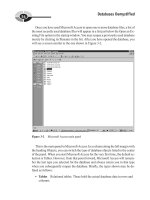
One of the common difficulties database users have with SQL Plus is that lines
that are too long to display wrap to new lines. Another is that the SQL statements
scroll off the screen when the results are displayed. Figure 4-2 provides an example
of these issues.
SQL Plus may be run from the Windows Command Shell using the following
command:
C:\>sqlplus hr/hrpass
When run this way, SQL Plus has all the same capabilities as the Windows GUI

version of SQL Plus, but is perhaps not as visually pleasing. In fact, it is exactly the
same utility program with only the user interface changed. An example of a com
-
mand run from the Windows Command Shell version of SQL Plus is shown in Fig
-
ure 4-3. This screen is quite similar to the one used when SQL Plus is run on other
platforms such as VMS VAX, Unix, and Linux.
Recognizing the need for a better user interface, Oracle developed SQL Plus
Worksheet as part of Oracle Enterprise Manager and started shipping it with
CHAPTER 4 Introduction to SQL
93
P:\010Comp\DeMYST\364-9\ch04.vp
Monday, February 09, 2004 9:03:16 AM
Color profile: Generic CMYK printer profile
Composite Default screen
94
Databases Demystified
Figure 4-1 DESCRIBE command output for the EMPLOYEES table
Figure 4-2 SQL Plus window with wrapped lines
P:\010Comp\DeMYST\364-9\ch04.vp
Monday, February 09, 2004 9:03:17 AM
Color profile: Generic CMYK printer profile
Composite Default screen
Oracle8i. When SQL Plus Worksheet is started from the Windows Start menu, the
login window appears, as shown here:
The Username and Password fields should be familiar from the SQL Plus discus
-
sion, and the Connect String field from SQL Plus is now called Service instead. The
Connect As field is for use by DBAs who require a special role (a named set of privi
-

leges) when they connect.
Once connected, the SQL Plus Worksheet panel appears, as shown in Figure 4-4.
SQL statements may be typed in the upper window, and the results are shown in the
lower window. The icons in the toolbar at the top of the left margin provide various
control functions, including disconnecting from the database, executing the current
SQL statement, scrolling back and forth through a history of recent statements, and
accessing the help facility.
CHAPTER 4 Introduction to SQL
95
Figure 4-3 SQL Plus window, command-line version
P:\010Comp\DeMYST\364-9\ch04.vp
Monday, February 09, 2004 9:03:17 AM
Color profile: Generic CMYK printer profile
Composite Default screen
The SQL Plus Worksheet panel is used for the presentation of the examples that
follow because of its superior formatting of query results.
Where’s the Data?
You probably noticed that although SQL Plus and SQL Plus Worksheet help you for
-
mat and run SQL statements, they don’t provide an easy way for you to see the names
and definitions of the database objects available to you. This is a typical arrangement
for an RDBMS. If you are not familiar with the database schema you are using, you
can obtain some basic information in one of two ways: through catalog views or a tool
such as the Oracle Enterprise Manager. Catalog views are special views provided by
the RDBMS that present database metadata that documents the database contents.
96
Databases Demystified
Figure 4-4 SQL Plus Worksheet panel
P:\010Comp\DeMYST\364-9\ch04.vp
Monday, February 09, 2004 9:03:17 AM

Color profile: Generic CMYK printer profile
Composite Default screen
Finding Database Objects Using Catalog Views
Oracle provides a comprehensive set of catalog views that may be queried to show
the names and definitions of all database objects available to a database user. Most
other RDBMSs have a similar capability, but of course the names of the views vary.
By issuing a SELECT statement against any of these views, you may display infor
-
mation about your database objects. Consult the Oracle Server Reference manual
(available from Oracle Technology Network website) for complete information on
the available catalog views. Here are two of the most useful ones:
•
USER_TABLES Contains one row of information for each table in the
user schema. This view contains a lot of columns, but the one of most interest,
TABLE_NAME, is the first column in the view. Once you know the table
names, the DESCRIBE command (already introduced) can be used on each
to show more information about the table definitions. Figure 4-5 shows an
example of selecting everything from the USER_TABLES view.
The SQL SELECT statement, shown in Figure 4-5, is described in more
detail a little further along in this chapter.
•
USER_VIEWS Contains one row of information for each view in the
user schema, containing, among other things, the name of the view and
the text of the SQL statement that forms the view.
CHAPTER 4 Introduction to SQL
97
Figure 4-5 Selecting from the USER_TABLES view
P:\010Comp\DeMYST\364-9\ch04.vp
Monday, February 09, 2004 9:03:17 AM
Color profile: Generic CMYK printer profile

Composite Default screen
98
Databases Demystified
Demystified / Databases Demystified / Oppel/ 225364-9 / Chapter 4
Viewing Database Objects Using
Oracle Enterprise Manager
For those less inclined to type SQL commands, Oracle provides a GUI tool known as
Oracle Enterprise Manager (OEM). Other RDBMS vendors provide similar tools, such
as the Enterprise Manager tool that comes with Sybase and Microsoft SQL Server.
The Oracle Enterprise Manager Console can be started from the Windows Start
menu, by choosing Start | Programs | Oracle - OraHome92 | Enterprise Manager
Console.
Once started, OEM presents a window asking whether it should be launched in
standalone mode or if instead you wish to log in to the Oracle management server.
Unless directed otherwise by your DBA, you should always launch OEM in
standalone mode. Next, the Oracle Enterprise Manager login window will be dis
-
played, as already shown in a previous illustration. For OEM to work perfectly, you
should connect to the database as the SYSTEM user. However, if you are working on
an employer’s database system, your DBA may not be very interested in handing
over the keys to the database to a beginner, so you may have to settle for signing in
with the Oracle database username provided by the DBA. If you do so, some error
messages related to privileges may appear, and some features may not work. Once
connected to OEM, you will see a panel similar to the one in Figure 4-6.
Here are the exact steps to follow to get to the EMPLOYEES table as shown in
Figure 4-6:
1. Start the OEM Console from the Start menu, as described earlier.
2. Select Launch Standalone on the Oracle Enterprise Manager Console login
window and then click OK.
3. Click the plus sign (+) next to Databases in the left column to expand the

list of databases.
4. Click the plus sign (+) next to the name of your Oracle database (ORA9I in
this example) to expand the list of database object types.
5. The Database Connect Information window will appear. In this window, type
SYSTEM in the Username field and type the password for the SYSTEM user
in the Password field. Click OK.
6. Click the plus sign (+) next to Schema to expand the list of schemas in the
database.
7. Click the plus sign (+) next to HR to expand the list of objects belonging to
the HR schema.
P:\010Comp\DeMYST\364-9\ch04.vp
Monday, February 09, 2004 9:03:18 AM
Color profile: Generic CMYK printer profile
Composite Default screen
8. Click the plus sign (+) next to Tables to expand the list of tables in the
HR schema.
9. Click the EMPLOYEES table to display its description in the right panel.
OEM is so full of features that describing them in detail would take an entire book
of at least this size. The feature you will be most interested in is the hierarchical tree
of databases and database objects that appears in the column along the left margin of
the panel. Expanding the Schema item shows all the schemas in the database (each
Oracle database user gets their own schema). Expanding any schema shows the ob
-
ject types available in that schema. Expanding any object type (as we did with the
Tables type) shows a list of objects of that type in the selected schema, and clicking
or expanding any individual object shows more information about that object (as we
did by clicking the EMPLOYEES table object).
You’ve seen a little bit of the SQL SELECT statement so far. In the next section
we take a detailed look at SQL.
CHAPTER 4 Introduction to SQL

99
Figure 4-6 Oracle Enterprise Manager Console
P:\010Comp\DeMYST\364-9\ch04.vp
Monday, February 09, 2004 9:03:18 AM
Color profile: Generic CMYK printer profile
Composite Default screen
100
Databases Demystified
Demystified / Databases Demystified / Oppel/ 225364-9 / Chapter 4
Data Query Language (DQL):
The SELECT Statement
The SELECT statement retrieves data from the database. The clauses of the state
-
ment, as demonstrated in the following sections, are as follows:
•
SELECT Lists the columns that are to be returned in the results
•
FROM Lists the tables or views from which data is to be selected
•
WHERE Provides conditions for the selection of rows in the results
•
ORDER BY Specifies the order in which rows are to be returned
•
GROUP BY Groups rows for various aggregate functions
Although it is customary in SQL to write keywords in upper case, this is not nec-
essary in most implementations. The RDBMS SQL interpreter will usually recog-
nize keywords written in upper, lower or mixed case. In Oracle SQL, all database
object names (tables, views, synonyms, etc.) may be written in any case, but Oracle
automatically changes them to upper case during processing because all Oracle da-
tabase object names are stored in upper case in Oracle’s metadata. Be careful with

other versions of SQL, however. For example, both Sybase and MS SQL Server can
be set to a case-sensitive mode where object names written in different cases are
treated as different objects. In case-sensitive mode, the following names would be
considered different tables: EMPLOYEES, Employees, employees.
Example 4-1: Listing All Employees
The asterisk (*) symbol may be used in place of a column list in order to select all
columns in a table or view. This is a useful feature for quickly listing data, but it
should be avoided in statements that will be reused because it compromises logical
data independence because any new column will be automatically selected the next
time the statement is run. Note also that in SQL syntax, tables, views, and synonyms
(an alias for a table or view) are all referenced in the same way. It should follow that
the names of these come for the same namespace, meaning that a name of a table, for
example, must be unique among all tables, views, and synonyms defined in particu
-
lar schema. Figure 4-7 shows the Example 4-1 SQL statement and its results.
Example 4-2: Limiting Columns to Display
To specify the columns to be selected, provide a comma-separated list following the
SELECT keyword. Keep in mind that the list actually provides expressions that
P:\010Comp\DeMYST\364-9\ch04.vp
Monday, February 09, 2004 9:03:18 AM
Color profile: Generic CMYK printer profile
Composite Default screen
describe the columns desired in the query results, and although many times these ex-
pressions are merely column names from tables or views, they may also be any con-
stant or formula that SQL can interpret and form into data values for the column. The
examples that follow show you how to use formulas and constants to form query col-
umns. Figure 4-8 shows the SQL for selecting the LAST_NAME, FIRST_NAME,
HIRE_DATE, and SALARY columns.
CHAPTER 4 Introduction to SQL
101

Figure 4-7 Example 4-1, “Listing All Employees”
Figure 4-8 Example 4-2, “Limiting Columns to Display”
P:\010Comp\DeMYST\364-9\ch04.vp
Monday, February 09, 2004 9:03:18 AM
Color profile: Generic CMYK printer profile
Composite Default screen
Example 4-3: Sorting Results
Just as in Microsoft Access, in SQL there is no guarantee as to the sequence of the
rows in the query results unless the desired sequence is specified in the query. In
SQL, providing a comma-separated list following the ORDER BY keyword does
this. Figure 4-9 shows the SQL from Figure 4-8 with row sequencing added.
Also note the following points:
•
Ascending sequence is the default for each column, but the keyword ASC
may be added after the column name for ascending sequence, and DESC may
be added for descending sequence.
•
The column(s) named in the ORDER BY list do not have to be included in
the query results (that is, the SELECT list). However, this is not the best
human engineering.
•
Instead of column names, the relative position of the columns in the results may
be listed. The number provided has no correlation with the column position in
the source table or view, however. This option is frowned upon in formal SQL
because someone changing the query at a later time might shuffle columns
around in the SELECT list and not realize that, in doing so, they are changing
the columns used for sorting results. In Example 4-3, the following ORDER
BY clause achieves the same query results: ORDER BY 1,2.
102
Databases Demystified

Figure 4-9 Example 4-3, “Sorting Results”
P:\010Comp\DeMYST\364-9\ch04.vp
Monday, February 09, 2004 9:03:19 AM
Color profile: Generic CMYK printer profile
Composite Default screen
Choosing Rows to Display
SQL uses the WHERE clause for the selection of rows to display. Without a
WHERE clause, all rows found in the source tables and/or views are displayed.
When a WHERE clause is included, the rules of Boolean algebra, named for logi
-
cian George Boole, are used to evaluate the WHERE clause for each row of data.
Only rows for which the WHERE clause evaluates to a logical “true” are displayed
in the query results.
As you will see in the examples that follow, individual tests of conditions must
evaluate to either “true” or “false.” The conditional operators supported are the same
ones shown in Chapter 3 in Example 3-7 (=, <, <=, >, >=, and <>). If multiple condi
-
tions are tested in a single WHERE clause, the outcomes of these conditions can be
combined together using logical operators such as AND, OR, and NOT. Parentheses
may be (and should be) added to complex statements for clarity and to control the or-
der in which the conditions are evaluated. A rather complicated order of precedence
is used when multiple logical operators appear in one statement. However, it is far
simpler to remember that conditions inside a pair of parentheses are always evalu-
ated first, and to simply include enough sets of parentheses so there can be no doubt
as to the order in which the conditions are evaluated.
Example 4-4: A Simple WHERE Clause
Figure 4-10 shows a simple WHERE clause that selects only rows where SALARY
is equal to 11000.
CHAPTER 4 Introduction to SQL
103

Figure 4-10 Example 4-4, “A Simple WHERE Clause”
P:\010Comp\DeMYST\364-9\ch04.vp
Monday, February 09, 2004 9:03:19 AM
Color profile: Generic CMYK printer profile
Composite Default screen
Example 4-5: The BETWEEN Operator
SQL provides the BETWEEN operator to assist in finding ranges of values. The end
points are included in the returned rows. Figure 4-11 shows the use of the
BETWEEN operator to find all rows where SALARY is greater than or equal to
10000 and SALARY is less than or equal to 11000. Here’s an alternative way to
write the equivalent WHERE clause:
WHERE SALARY >= 10000
AND SALARY <= 11000
Example 4-6: The LIKE Operator
For searching character columns, SQL provides the LIKE operator, which compares
the character string in the column to a pattern, returning a logical “true” if the col
-
umn matches the pattern, and “false” if not. The underscore character ( _ ) may be
used as a positional wildcard, meaning it matches any character in that position of
the character string being evaluated. The percent sign (%) may be used as a
nonpositional wildcard, meaning it matches any number of characters for any
length. Note that Microsoft Access has a similar feature, but the wildcard characters
are different (they match those in DOS and Visual Basic): The question mark (?) is
the positional wildcard, and the asterisk (*) is the nonpositional wildcard. The fol
-
lowing table provides some examples:
104
Databases Demystified
Figure 4-11 Example 4-5, “The BETWEEN Operator”
P:\010Comp\DeMYST\364-9\ch04.vp

Monday, February 09, 2004 9:03:19 AM
Color profile: Generic CMYK printer profile
Composite Default screen
Pattern Interpretation
%Now Matches any character string that ends with “Now”
Now% Matches any character string that begins with “Now”
%Now% Matches any character string that contains “Now” (whether at the beginning, the
end, or in the middle)
N_w Matches any string of exactly three characters, where the first character is “N” and
the third character is “w”
%N_w% Matches any string that contains the character “N” followed by any character,
which is in turn followed by the character “w” and continues with any number
of characters
Figure 4-12 shows the use of the LIKE operator to display only rows where the
FIRST_NAME column starts with the text “Pete”.
Example 4-7: Compound Conditions Using OR
As stated earlier, multiple conditions may be combined using the OR operator. Fig
-
ure 4-13 shows a WHERE clause that selects rows having either a FIRST_NAME
column beginning with “Pete” or a SALARY column that is between 10000 and
20000 inclusive.
Figure 4-14 changes the OR operator from Example 4-6 to the AND operator.
Note that only one row is returned now because both conditions must be true for a row
to appear in the query results.
CHAPTER 4 Introduction to SQL
105
Figure 4-12 Example 4-6, “The LIKE Operator”
P:\010Comp\DeMYST\364-9\ch04.vp
Monday, February 09, 2004 9:03:19 AM
Color profile: Generic CMYK printer profile

Composite Default screen
Example 4-8: The Subselect
A very powerful feature of SQL is the subselect (or subquery), which, as the name
implies, refers to a SELECT statement that contains a subordinate SELECT state
-
ment. This can be a very flexible way of selecting data.
Let’s assume that we want to list all employees who work in sales. The dilemma is
that the DEPARTMENTS table in the sample HR schema contains several sales de
-
partments, including Sales, Government Sales, and Retail Sales. We could place liter
-
als for those three department names or their corresponding department IDs in the
WHERE clause of our SELECT statement. However, the problem we then face is
maintenance of the query if a sales-related department is subsequently added or elimi
-
nated. A safer approach is to use an SQL query to find the applicable department IDs
106
Databases Demystified
Figure 4-13 Example 4-7, “Compound Conditions Using OR”
Figure 4-14 Example 4-7, “Compound Conditions Using AND”
P:\010Comp\DeMYST\364-9\ch04.vp
Monday, February 09, 2004 9:03:19 AM
Color profile: Generic CMYK printer profile
Composite Default screen
when the query is run and then use that list of IDs to find the employees. The query to
find the department IDs is simple enough:
SELECT DEPARTMENT_ID
FROM DEPARTMENTS
WHERE DEPARTMENT_NAME LIKE '%Sales%';
If we place the preceding SELECT statement in the WHERE clause of a query that

lists the employee information of interest, we arrive at the query shown in Figure 4-15.
Note that SQL syntax requires the subselect to be enclosed in a pair of parentheses.
The statement shown in Example 4-8 is known as a noncorrelated subselect be
-
cause the inner SELECT (that is, the one inside the WHERE clause) can be run first
and the results used when the outer SELECT is run. There also is such a thing as a
correlated subselect (or subquery), where the outer query must be invoked multiple
times, once for each row found in the inner query. Consider this example:
SELECT LAST_NAME, FIRST_NAME, SALARY, DEPARTMENT_ID
FROM EMPLOYEES A
WHERE SALARY >
(SELECT AVG(SALARY)
FROM EMPLOYEES B
WHERE A.DEPARTMENT_ID = B.DEPARTMENT_ID);
This statement finds all employees whose salary is above the average salary for their
department. The inner SELECT finds the average salary for each department. The outer
SELECT is then executed for each row returned from the inner SELECT (that is, for
each department) to find all employees for that department where the salary is above the
CHAPTER 4 Introduction to SQL
107
Figure 4-15 Example 4-8, “The Subselect”
P:\010Comp\DeMYST\364-9\ch04.vp
Monday, February 09, 2004 9:03:20 AM
Color profile: Generic CMYK printer profile
Composite Default screen
average for that department. Hopefully, you recognized the AVG function, which was
introduced back in Chapter 3 in Example 3-12. We will review using aggregate func
-
tions in an upcoming SQL example.
Joining Tables

Example 4-9: The Cartesian Product
As you learned previously in Example 3-8, we need to join tables (or views) whenever
we need data from more than one table in our query results. In SQL, you specify joins
by listing the tables or views to be joined in a comma-separated list in the FROM
clause of the SELECT statement. However, SQL is not going to remind you to tell the
RDBMS how to match rows in the tables (or views) being joined. If you forget, you
will get a Cartesian product, as shown in Figure 4-16.
Whenever you write a new query, you should apply a “reasonableness” test to the
results. Example 4-9 looks fine on the surface, but when you consider that there are
only 107 employees, you realize something is horribly wrong. How could we possibly
108
Databases Demystified
Figure 4-16 Example 4-9, “The Cartesian Product”
P:\010Comp\DeMYST\364-9\ch04.vp
Monday, February 09, 2004 9:03:20 AM
Color profile: Generic CMYK printer profile
Composite Default screen
get 2889 rows simply by joining employees and departments? The answer: We failed
to include a join specification in the WHERE clause, so the RDBMS created a Carte
-
sian product for us, joining each employee with every department, and 27 departments
times 107 employees yields 2889 (27 * 107) rows. Oops!
Example 4-10: The Inner Join of Two Tables
Figure 4-17 shows the correction, which involves adding a WHERE clause that tells
the DBMS to match the DEPARTMENT_ID column in the EMPLOYEES table (the
foreign key) to the DEPARTMENT_ID column in the DEPARTMENTS table (the pri
-
mary key). Now we get a much more reasonable result with 106 rows.
However, if there are 107 employees, why did we only get 106 in Example 4-10?
The answer lies in the fact that we performed an inner (or standard) join. Rows were

returned only when a matching department row was found for an employee—and
there is one employee, the owner of the company, who does not work in a depart
-
ment. We can correct this problem by changing our inner join to an outer join. In this
case, we want all rows from the EMPLOYEES table, even if no matching row is
found in the DEPARTMENTS table for some employees.
CHAPTER 4 Introduction to SQL
109
Figure 4-17 Example 4-10, “Inner Join of Two Tables”
P:\010Comp\DeMYST\364-9\ch04.vp
Monday, February 09, 2004 9:03:20 AM
Color profile: Generic CMYK printer profile
Composite Default screen
Example 4-11: Outer Joins in Oracle
The Oracle syntax for outer joins is just plain strange. It involves placing a plus sign
enclosed in parentheses (+) in the WHERE clause on the side of the condition where
null values are to be returned. In this case, when there is no matching
DEPARTMENTS table row for an employee, we want the data from the
EMPLOYEES table to display anyway, with the DEPARTMENT_NAME from the
DEPARTMENTS table set to null. If you think of the symbol (+) as meaning “add
nulls here,” you might find it easier to remember. Here is the adjusted SQL statement:
SELECT EMPLOYEE_ID, LAST_NAME, FIRST_NAME, DEPARTMENT_NAME
FROM EMPLOYEES, DEPARTMENTS
WHERE EMPLOYEES.DEPARTMENT_ID = DEPARTMENTS.DEPARTMENT_ID(+);
The Oracle outer join syntax grew out of necessity, with customers demanding a
solution and no standards at the time to follow. Starting with Oracle9i Release 2, the
ANSI Standard LEFT OUTER JOIN syntax is supported. So now the preceding
statement may be rewritten in a more understandable way:
SELECT EMPLOYEE_ID, LAST_NAME, FIRST_NAME, DEPARTMENT_NAME
FROM EMPLOYEES

LEFT OUTER JOIN DEPARTMENTS
ON EMPLOYEES.DEPARTMENT_ID = DEPARTMENTS.DEPARTMENT_ID;
Example 4-12: Limiting Join Results
Additional conditions can easily be added to the WHERE clause to limit rows re
-
turned from a query that also involves joins. Figure 4-18 shows a modification to
110
Databases Demystified
Figure 4-18 Example 4-12, “Limiting Join Results”
P:\010Comp\DeMYST\364-9\ch04.vp
Monday, February 09, 2004 9:03:20 AM
Color profile: Generic CMYK printer profile
Composite Default screen
Example 4-10, such that only employees who work in departments with “Sales” in
the department name are retuned.
Example 4-13: The Self-Join
When a table has a recursive relationship, we need to join the table to itself in order to
follow the relationship in our query results. The EMPLOYEES table has such a rela
-
tionship in that the MANAGER_ID column contains the EMPLOYEE_ID value of
the employee to whom each employee reports. In our example, every employee has a
manager in the table except for the owner of the company, as shown in Figure 4-19.
Note that we added another wrinkle to this example by concatenating the first and
last names of the manager with a space in between to form the MANAGER_NAME
column in the results. The column name is assigned using the keyword AS followed
by the desired name. The query was coded as an inner join, so the one employee who
does not have a manager will not show up in the results. As with any join, we can re
-
write this one into an outer join by changing the WHERE clause. In this example, it
would be written as follows:

WHERE A.MANAGER_ID = B.MANAGER_ID (+)
CHAPTER 4 Introduction to SQL
111
Figure 4-19 Example 4-13, “The Self-Join”
P:\010Comp\DeMYST\364-9\ch04.vp
Monday, February 09, 2004 9:03:21 AM
Color profile: Generic CMYK printer profile
Composite Default screen
Aggregate Functions
Example 4-14: Simple Aggregate Functions
As you will recall from Example 3-12 in the previous chapter, aggregate functions
combine multiple rows together. In Figure 4-20, aggregate functions are used to find
the minimum, maximum, and average salaries for all employees along with a count
of the total number of employees. Because there is no GROUP BY clause to group
rows, the entire table is considered one group, so only one row is returned in the
result set.
Example 4-15: Mixed Aggregate and
Normal Columns (Error)
If we add DEPARTMENT_ID to the query without adding a GROUP BY clause,
the query returns an error message, as shown in Figure 4-21. The error message can
be confusing, but notice the placement of the asterisk under the SQL statement. Ora
-
cle is attempting to show the particular part of the statement where the error was
found. In this case, it is telling you that DEPARTMENT_ID is not a group function.
Example 4-16: Aggregate Functions with GROUP BY
The request in Example 4-15 is illogical because it essentially asks the RDBMS to
display every value of DEPARTMENT_ID, but at the same time, display only one
row containing the values for the other columns (those columns being formed with
aggregate functions). To remedy the situation, we must tell the RDBMS that we
112

Databases Demystified
Figure 4-20 Example 4-14, “Simple Aggregate Functions”
P:\010Comp\DeMYST\364-9\ch04.vp
Monday, February 09, 2004 9:03:21 AM
Color profile: Generic CMYK printer profile
Composite Default screen
wish to group the rows by DEPARTMENT_ID, and for each group display the
DEPARTMENT_ID along with the aggregate column results (the minimum, maxi-
mum, and average salaries for the department and the count of the number of em-
ployees in the department). The corrected statement is shown in Figure 4-22. We add
a ROUND function to the AVG(SALARY) column to round the average to two deci-
mal places. Note that the ROUND function is not an aggregate function—it merely
rounds a single column value. It is perfectly acceptable to apply a function to the re-
sults of another function, which is known as nesting functions. There seems no limit
to the clever things we can do with SQL.
CHAPTER 4 Introduction to SQL
113
Figure 4-21 Example 4-15, “Mixed Aggregate and Normal Columns (Error)”
Figure 4-22 Example 4-16, “Aggregate Functions with GROUP BY”
P:\010Comp\DeMYST\364-9\ch04.vp
Monday, February 09, 2004 9:03:21 AM
Color profile: Generic CMYK printer profile
Composite Default screen
The GROUP BY clause causes returned rows to be automatically ordered by the col
-
umns listed because the DBMS must perform a sort in order to group the rows. However,
an ORDER BY may also be included to return the rows in an alternate sequence. If the
ORDER BY clause must include calculated columns, just use the expression for the col
-
umn—you cannot use any alias name for the column because the alias is assigned to the

column in the query results and therefore does not exist at the time the query runs.
Data Manipulation Language (DML)
The DML statement types in SQL are INSERT, UPDATE, and DELETE. These
commands allow you to add, change, and remove rows of data in the tables. Before
we look at each of these statement types, you first need to understand the concept of
transactions and how the RDBMS supports them.
Transaction Support (COMMIT and ROLLBACK)
In terms of the RDBMS, a transaction is a series of one or more SQL statements that
are treated as a single unit. A transaction must completely work or completely fail,
meaning that any database changes a transaction makes must be made permanent
when the transaction successfully completes. On the other hand, these changes must
be entirely removed from the database if the transaction fails before completion. For
example, we could start a transaction at the beginning of a process that creates a new
order and then, at the end of the process when all the order information has been en
-
tered, completes the transaction. It is important that other database users not see frag
-
ments of an incomplete order until it has been completely entered and confirmed.
SQL provides support for transactions with the COMMIT and ROLLBACK
statements. There is some variation in the syntax and handling of these commands
across different RDBMS vendors. Most vendors require no argument with the
COMMIT or ROLLBACK statement, so the statement is just the keyword followed
by the semicolon that ends every SQL statement.
In Oracle, a transaction is automatically started for each database user session as soon
as the user connects to the database. At any time, the database user can issue a
COMMIT, which makes all the database changes completed up to that point permanent
and therefore visible to any other database user. The user can also issue a ROLLBACK,
which reverses any changes made to the database. The COMMIT and ROLLBACK
statements not only end one transaction, but they also begin a new one. There is one
more wrinkle to remember: In Oracle, an automatic commit occurs before any DDL

statement. (DDL statements are covered later in this chapter.)
114
Databases Demystified
P:\010Comp\DeMYST\364-9\ch04.vp
Monday, February 09, 2004 9:03:21 AM
Color profile: Generic CMYK printer profile
Composite Default screen
By contrast, in Sybase and Microsoft SQL Server, transaction support is not as
automatic. The database user must issue a BEGIN TRANSACTION statement to
start a transaction. Once a transaction is started, changes made to the database can be
made permanent with a COMMIT TRANSACTION statement, or they can be re
-
versed using a ROLLBACK TRANSACTION statement. Some RDBMSs, such as
Microsoft Access and MySQL, do not provide transaction support at all.
The INSERT Statement
The INSERT statement in SQL is used to add new rows of data to tables. An INSERT
statement may also insert rows via a view, provided the following conditions are met:
•
If the view joins multiple tables, the columns referenced by the INSERT
statement must all be from the same table. Said another way, an INSERT can
only affect one table.
•
The view must include all the mandatory table columns in the base table.
If there are columns with NOT NULL constraints that do not appear in the
view, it is impossible to provide values for those columns and therefore
impossible to use the view to perform an insert.
The INSERT statement takes two basic forms: one where column values are pro-
vided in the statement itself, and the other where values are selected from a table or
view using a subselect. Let’s have a look at those two forms.
Example 4-17: INSERT with VALUES Clause

The INSERT with VALUES clause form of the INSERT statement can only create
one row each time it is run because the values for that one row of data are provided in
the statement itself. Figure 4-23 shows an example.
CHAPTER 4 Introduction to SQL
115
Figure 4-23 Example 4-17, “INSERT with VALUES Clause”
P:\010Comp\DeMYST\364-9\ch04.vp
Monday, February 09, 2004 9:03:22 AM
Color profile: Generic CMYK printer profile
Composite Default screen