Designing and Implementing Linux Firewalls and QoS using netfilter, iproute2, NAT, and filter phần 4 docx

Chapter 3
[ 75 ]
OPTIONS := { -V[ersion] | -s[tatistics] | -r[esolve] |
-f[amily] { inet | inet6 | ipx | dnet | link } |
-o[neline] }
root@router:~#
The ip link command shows the network device's congurations that can be
changed with ip link set. This command is used to modify the device's proprieties
and not the IP address.
The IP addresses can be congured using the ip addr command. This command can
be used to add a primary or secondary (alias) IP address to a network device (ip
addr add), to display the IP addresses for each network device (ip addr show), or to
delete IP addresses from interfaces (ip addr del). IP addresses can also be ushed
using different criteria, e.g. ip addr flush dynamic will ush all routes added to the
kernel by a dynamic routing protocol.
Neighbor/Arp table management is done using ip neighbor, which has a few
commands expressively named add, change, replace, delete, and flush.
ip tunnel is used to manage tunneled connections. Tunnels can be gre, ipip, and
sit. We will include an example later in the book on how to build IP tunnels.
The ip tool offers a way for monitoring routes, addresses, and the states of devices
in real-time. This can be accomplished using ip monitor, rtmon, and rtacct
commands included in the iproute2 package.
One very important and probably the most used object of the ip tool is ip route,
which can do any operations on the kernel routing table. It has commands to add,
change, replace, delete, show, ush, and get routes.
One of the things iproute2 introduced to Linux that ensured its popularity was
policy routing. This can be done using ip rule and ip route in a few simple steps.
Trafc Control: tc
The tc command allows administrators to build different QoS policies in their
networks using Linux instead of very expensive dedicated QoS machines. Using
Linux, you can implement QoS in all the ways any dedicated QoS machine can and

even more. Also, one can make a bridge using a good PC running Linux that can be
transformed into a very powerful and very cheap dedicated QoS machine.
For that, QoS support must be congured in the Linux kernel (CONFIG_NET_QOS="Y"
and CONFIG_NET_SCHED="Y").
Firewall Prerequisites: netlter and iproute2
[ 76 ]
Queuing Packets
First of all, queuing is used to determine the way data is sent; so with queuing, we
can control how much data is sent, and with what priority we send data that matches
some criteria.
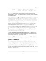
Please keep in mind that there is no way to queue incoming data. When we talk
about limiting upload and download speeds for some IP address, for example, we
talk about limiting the data our Linux router sends to that IP address on the interface
that IP address is connected to (download) and the data our Linux router sends over
the Internet from that IP address (upload), as in the following gure:
This is quite satisfying because TCP has ow control, which actually negotiates
the speed of the packet ow between two communicating hosts depending on the
capabilities of each host. UDP doesn't have ow control, but most of the applications
that use UDP as transport protocol implement ow control within themselves.
Well, things look pretty good, but this is how things work in the "perfect world",
where there aren't people with bad intentions (or stupid people without bad
intentions) that generate ood attacks because we can't limit the incoming data.
So, what's the problem? Well, put 99 computers near the 1.1.1.1 computer in the
earlier gure! Let's say there are 100 users on a FastEthernet connection (with more
switches, as the router has one Ethernet cable in one switch). We can limit each
computer to 1Mbps upload / 1Mbps download; so we're using 100 Mbps when
everyone is on the top of their limits. Now, if 1.1.1.1 wants to disrupt service to the
other users, it's very simple. Because there is no way of limiting incoming trafc,
if 1.1.1.1 oods one or many random hosts on the Internet with a 100Mbps data
stream, the router limits the outgoing data from 1.1.1.1 to 1Mbps, but it still receives

100Mbps on its eth1 interface. This results in denial of service, and there isn't really
much to do about it. If the switches are unmanaged, the only thing you can do about
it is to plug out the cable from the port in which 1.1.1.1 is connected.
Chapter 3
[ 77 ]
Now, to get back to the subject, queuing disciplines are of two kinds: classless
and classful.
Classless Queuing Disciplines (Classless qdiscs)
Classless qdiscs are the simplest ones because they only accept, drop, delay or
reschedule data. They can be attached to one interface and can only shape the
entire interface.
There are several qdisc implementations on Linux, most of them included in the
Linux kernel.
FIFO (pfo and bfo): The simplest qdisc, which functions by the First In,
First Out rule. FIFO algorithms have a queue size limit (buffer size), which
can be dened in packets for pfo or in bytes for bfo.
pfo_fast: The default qdisc on all Linux interfaces. It's important to know
how pfo_fast works; so we'll explain it soon.
Token Bucket Filter (tbf): A simple qdisc that is perfect for slowing down an
interface to a specied rate. It can allow short bursts over the specied rate
and is very processor friendly.
Stochastic Fair Queuing (SFQ): One of the most widely used qdiscs. SFQ
tries to fairly distribute the transmitting data among a number of ows.
Enhanced Stochastic Fair Queuing (ESFQ): Not included in the Linux
kernel, it works in the same manner as SFQ with the exception that the user
can control more of the algorithm's parameters such as depth (ows) limit,
hash table size options (hardcoded in original SFQ) and hash types.
Random Early Detection and Generic Random Early Detection (RED and
GRED): qdiscs suitable for backbone data queuing, with data rates over
100 Mbps.

There are more qdiscs than the ones I have stated here. However, from my experience,
SFQ and ESFQ do a great job, and are the qdiscs that I have got the best results with.
As I said earlier, the default qdisc on Linux for all interfaces is pfo_fast. Normally,
one would think that this is just like pfo, meaning there is a buffer and packets
pass through the buffer using the First In First Out rule. Actually, it's not quite true.
pfo_fast has 3 bands—0, 1, and 2—in which packets are placed according to their
TOS byte. Packets are sent out from those bands as follows:
Packets in the 0 band have the highest priority
Packets in the 1 band are sent out only if there aren't any packets in
the 0 band
•
•
•
•
•
•
•
•
Firewall Prerequisites: netlter and iproute2
[ 78 ]
Packets in the 2 band have the lowest priority and are sent out only if there
aren't any packets in the 0 and 1 bands.
It's important to know this because this can be a way to optimize how packets travel
through the network interfaces of our Linux routers. The TOS byte looks like this:
0 1 2 3 4 5 6 7
PRECEDENCE Type of Service — TOS MBZ
The TOS bits are dened as follows:
0000 Normal Service
0001 Minimize Monetary Cost (MMC)
0010 Maximize Reliability (MR)

0100 Maximize throughput (MT)
1000 Minimize Delay (MD)
Based on the TOS byte, the packets are placed in one of the three bands as follows:
•
•
•
•
•
•
Chapter 3
[ 79 ]
This means that, by default, Linux is smart enough to prioritize trafc according to
the TOS bytes. Usually, applications like Telnet, FTP, SMTP modify the TOS byte
to work in an optimal way. We will see later in this book how to optimize the
trafc ourselves.
Classful Queuing Disciplines
These qdiscs are used for shaping different types of data. The commonly used
classful qdiscs are CBQ (Class Based Queuing) and HTB (Hierarchical Token Bucket).
First of all, we need to learn how classful queuing disciplines work. The whole
process is not difcult; so I'll try to explain it as simply as possible.
Everything is based on a hierarchy. First, every interface has one root qdisc that
talks to the kernel. Second, there is a child class attached to the root qdisc. The child
class further has child classes that have qdiscs attached to schedule the data and leaf
classes, which are child classes of the child classes.
All confused? Have a look at the following image, which will explain away
the confusion:
So, basically CBQ or HTB qdiscs allow us to create child CBQ or HTB classes, which
we can set up to shape some kind of data. For each child class, we can attach a qdisc
for scheduling packets within that child class. Next, we can create leaf classes, which
are child classes of the qdiscs we attached to the child classes, or we can create leaf

classes as child classes' child classes attached to the root qdisc.
Firewall Prerequisites: netlter and iproute2
[ 80 ]
tc qdisc, tc class, and tc lter
To build the tree conguration in the earlier gure, we need to use the tc command:
tc qdisc manipulates queuing disciplines.
tc class manipulates classes.
tc filter manipulates lters used to identify data.
Both CBQ and HTB have a few parameters that can be adjusted to optimize
their performance. Throughout this book we will use different values to suit
the applications we are building. There is a lot of tuning to be done with these
parameters, and I'm not going to explain all of them as there are some that you will
probably never need.
CBQ qdiscs and classes have the following parameters:
root@router:~# tc qdisc add cbq help
Usage: cbq bandwidth BPS avpkt BYTES [ mpu BYTES ]
[ cell BYTES ] [ ewma LOG ]
root@router:~# tc class add cbq help
Usage: cbq bandwidth BPS rate BPS maxburst PKTS [ avpkt BYTES ]
[ minburst PKTS ] [ bounded ] [ isolated ]
[ allot BYTES ] [ mpu BYTES ] [ weight RATE ]
[ prio NUMBER ] [ cell BYTES ] [ ewma LOG ]
[ estimator INTERVAL TIME_CONSTANT ]
[ split CLASSID ] [ defmap MASK/CHANGE ]
and HTB qdiscs and classes' parameters are:
root@router:~# tc class add htb help
Usage: qdisc add htb [default N] [r2q N]
default minor id of class to which unclassified packets are sent {0}
r2q DRR quantums are computed as rate in Bps/r2q {10}
debug string of 16 numbers each 0-3 {0}

class add htb rate R1 [burst B1] [mpu B] [overhead O]
[prio P] [slot S] [pslot PS]
[ceil R2] [cburst B2] [mtu MTU] [quantum Q]
rate rate allocated to this class (class can still borrow)
burst max bytes burst which can be accumulated during idle
period {computed}
mpu minimum packet size used in rate computations
overhead per-packet size overhead used in rate computations
ceil definite upper class rate (no borrows) {rate}
cburst burst but for ceil {computed}
mtu max packet size we create rate map for {1600}
•
•
•
Chapter 3
[ 81 ]
prio priority of leaf; lower are served first {0}
quantum how much bytes to serve from leaf at once {use r2q}
TC HTB version 3.3
I will try to explain a few of these parameters while using them in the actual example
that follows.
Filters are used to identify the data we need to shape. We can identify the data
based on the way the rewall marked it using the fw classier, based on elds of the
IP header using the u32 classier, based on the kernel's routing decision using the
route classier, or based on RSVP using rsvp or rsvp6 classiers.
The tc filter command has the following parameters:
root@router:~# tc filter help
Usage: tc filter [ add | del | change | get ] dev STRING
[ pref PRIO ] [ protocol PROTO ]
[ estimator INTERVAL TIME_CONSTANT ]

[ root | classid CLASSID ] [ handle FILTERID ]
[ [ FILTER_TYPE ] [ help | OPTIONS ] ]
tc filter show [ dev STRING ] [ root | parent CLASSID ]
Where:
FILTER_TYPE := { rsvp | u32 | fw | route | etc. }
FILTERID := format depends on classifier, see there
OPTIONS := try tc filter add <desired FILTER_KIND> help
The most used classier is u32, because most people desire to identify data by IP
addresses, source or destination ports, etc. However, we will use the fw classier
along with u32 throughout the book. The u32 parameters are:
root@router:~# tc filter add u32 help
Usage: u32 [ match SELECTOR ] [ link HTID ] [ classid CLASSID
]
[ police POLICE_SPEC ] [ offset OFFSET_SPEC ]
[ ht HTID ] [ hashkey HASHKEY_SPEC ]
[ sample SAMPLE ]
or u32 divisor DIVISOR
Where: SELECTOR := SAMPLE SAMPLE
SAMPLE := { ip | ip6 | udp | tcp | icmp | u{32|16|8} } SAMPLE_ARGS
FILTERID := X:Y:Z
Firewall Prerequisites: netlter and iproute2
[ 82 ]
And for the fw classier:
root@router:~# tc filter add fw help
Usage: fw [ classid CLASSID ] [ police POLICE_SPEC ]
POLICE_SPEC := look at TBF
CLASSID := X:Y
A Real Example
In the following example we will try to divide a 10Mbps bandwidth between three
entities: a home-user, an ofce, and another ISP, as shown in the following gure:

Let's assume we want to give the home user 1Mbps of our bandwidth, the ofce
4Mbps, and the ISP 5Mbps.
First, let's see how this looks using CBQ. First, we need to add the root qdisc to the
eth1 interface on which the clients are connected:
tc qdisc add dev eth1 root handle 10: cbq bandwidth 100Mbit avpkt 1000
So, the command used is tc qdisc add with the dev parameter set to eth1 to
dene the interface we will attach the qdisc to. The root parameter species that this
is the root qdisc. We will assign handle 10 for the root qdisc. After specifying
Chapter 3
[ 83 ]
the handle, we specied cbq as the type of the qdisc, followed by the parameters for
cbq. bandwidth is set to 100Mbit, which is the physical bandwidth of the device, and
avpkt, which species the average packet size is set to 1000.
Next, we need to create a child class that will be the parent of all classes. This class
will have the bandwidth parameter equal to that of the root qdisc, equal to the
physical bandwidth of the interface:
tc class add dev eth1 parent 10:0 classid 10:10 cbq bandwidth 100Mbit
rate \
100Mbit allot 1514 weight 10Mbit prio 5 maxburst 20 avpkt 1000
bounded
For the child classes, we need to specify the parent class, which in this case is 10:0—
the root class. classid species the ID of the class, and bandwidth is the physical
bandwidth of the interface (100Mbit). The speed limit is specied with the rate
parameter, followed by the rate in bits (in this case, 100Mbit). The allot parameter
is the base unit for how much data the class can send in one round. weight is a
parameter used by CBQ with allot to calculate how much data is sent in one round.
Actually, from our experience and tests, weight pretty much species the rate in
bytes for the class.
We will be using in this book parameters that gave the
best results in our tests. Except bandwidth, rate, and

weight, we don't recommend learning about all the other
parameters. However, there is a more detailed explanation
at: />classful.html#AEN939.
For each client, we will create leaf classes, qdiscs, and lters. Let's start with the
home user:
tc class add dev eth1 parent 10:10 classid 10:100 cbq bandwidth
100Mbit rate \
1Mbit allot 1514 weight 128Kbit prio 5 maxburst 20 avpkt 1000
bounded
tc qdisc add dev eth1 parent 10:100 sfq quantum 1514b perturb 15
tc filter add dev eth1 parent 10:0 protocol ip prio 5 u32 match ip dst
1.1.1.1 flowid 10:100
So we created the 10:100 class with a rate of 1Mbit and 128Kbit weight. Next, we
attached an sfq qdisc and a u32 lter to match all trafc with the destination IP
address 1.1.1.1. The bounded argument of the tc class add cbq command means
Firewall Prerequisites: netlter and iproute2
[ 84 ]
that the class isn't allowed to borrow bytes from other classes, meaning that there is
no way that data for this class will go over 1Mbps.
A lot of documentation explains that weight should be
rate/10. In our case, weight would be 100Kbit and the
user wouldn't get data with speed above 100KB/s which is
not 1Mbps. We've been always using weight as rate/8
because this seems more fair to me.
Now, the other classes, qdiscs, and lters look like this:
#the office
tc class add dev eth1 parent 10:10 classid 10:200 cbq bandwidth
100Mbit rate \
4Mbit allot 1514 weight 512Kbit prio 5 maxburst 20 avpkt 1000
bounded

tc qdisc add dev eth1 parent 10:200 sfq quantum 1514b perturb 15
tc filter add dev eth1 parent 10:0 protocol ip prio 5 u32 match ip dst
1.1.2.0/24 flowid 10:200
#the ISP
tc class add dev eth1 parent 10:10 classid 10:300 cbq bandwidth
100Mbit rate \
5Mbit allot 1514 weight 640Kbit prio 5 maxburst 20 avpkt 1000
bounded
tc qdisc add dev eth1 parent 10:300 sfq quantum 1514b perturb 15
tc filter add dev eth1 parent 10:0 protocol ip prio 5 u32 match ip dst
1.1.1.2 flowid 10:300
tc filter add dev eth1 parent 10:0 protocol ip prio 5 u32 match ip dst
1.1.3.0/24 flowid 10:300
As you can see in the ISP case, we can add as many lters as we want to a class.
To verify the conguration, we can use tc class show dev eth1 and see the classes:
root@router:~# tc class show dev eth1
class cbq 10: root rate 100000Kbit (bounded,isolated) prio no-transmit
class cbq 10:100 parent 10:10 leaf 806e: rate 1000Kbit (bounded) prio 5
class cbq 10:10 parent 10: rate 100000Kbit (bounded) prio 5
class cbq 10:200 parent 10:10 leaf 806f: rate 4000Kbit (bounded) prio 5
class cbq 10:300 parent 10:10 leaf 8070: rate 5000Kbit (bounded) prio 5
Chapter 3
[ 85 ]
Now, to see that a class is actually shaping packets, we send three ping packets to
1.1.1.1, and check to see if the CBQ class matched those packets using tc –s class
show dev eth1:
root@router:~# tc -s class show dev eth1 | fgrep -A 2 10:100
class cbq 10:100 parent 10:10 leaf 806e: rate 1000Kbit (bounded) prio 5
Sent 294 bytes 3 pkts (dropped 0, overlimits 0)
borrowed 0 overactions 0 avgidle 184151 undertime 0

Now everything looks OK; so let's move on to HTB. Before we do that, we need to
delete the CBQ root qdisc using:
root@router:~# tc qdisc del root dev eth1
Using HTB looks a bit simpler than CBQ. First, the root qdisc looks like this:
tc qdisc add dev eth1 root handle 10: htb
Next, we will create the child class:
tc class add dev eth1 parent 10:0 classid 10:10 htb rate 100Mbit
Now, the qdiscs and lters within the client classes are the same as in the CBQ
example. The only thing that differs is how the classes are built. Let's see the
home-user class, qdisc, and lter:
tc class add dev eth1 parent 10:10 classid 10:100 htb rate 1Mbit
tc qdisc add dev eth1 parent 10:100 sfq quantum 1514b perturb 15
tc filter add dev eth1 protocol ip parent 10:0 prio 5 u32 match ip dst
1.1.1.1 flowid 10:100
So much simple, isn't it? Let's create the other two entities' classes, qdiscs, and lters:
#the office
tc class add dev eth1 parent 10:10 classid 10:200 htb rate 4Mbit
tc qdisc add dev eth1 parent 10:200 sfq quantum 1514b perturb 15
tc filter add dev eth1 parent 10:0 protocol ip prio 5 u32 match ip dst
1.1.2.0/24 flowid 10:200
#the ISP
tc class add dev eth1 parent 10:10 classid 10:300 htb rate 5Mbit
tc qdisc add dev eth1 parent 10:300 sfq quantum 1514b perturb 15
tc filter add dev eth1 parent 10:0 protocol ip prio 5 u32 match ip dst
Firewall Prerequisites: netlter and iproute2
[ 86 ]
1.1.1.2 flowid 10:300
tc filter add dev eth1 parent 10:0 protocol ip prio 5 u32 match ip dst
1.1.3.0/24 flowid 10:300
Now it's time to verify the conguration using tc class show dev eth1:

root@router:~# tc class show dev eth1
class htb 10:10 root rate 100000Kbit ceil 100000Kbit burst 126575b
cburst 126575b
class htb 10:100 parent 10:10 leaf 8072: prio 0 rate 1000Kbit ceil
1000Kbit burst 2849b cburst 2849b
class htb 10:200 parent 10:10 leaf 8073: prio 0 rate 4000Kbit ceil
4000Kbit burst 6599b cburst 6599b
class htb 10:300 parent 10:10 leaf 8074: prio 0 rate 5000Kbit ceil
5000Kbit burst 7849b cburst 7849b
and after sending three ping packets to 1.1.1.1, we should see them on the 10:100 class:
root@router:~# tc -s class show dev eth1 | fgrep -A 4 10:100
class htb 10:100 parent 10:10 leaf 8072: prio 0 rate 1000Kbit ceil
1000Kbit burst 2849b cburst 2849b
Sent 294 bytes 3 pkts (dropped 0, overlimits 0)
rate 24bit
lended: 3 borrowed: 0 giants: 0
tokens: 18048 ctokens: 18048
There is no catch in all of this—HTB looks simpler and it
really is. CBQ has more parameters that can be adjusted
by the user, while HTB does much of the adjustments
internally.
Summary
This chapter introduced netlter/iptables and iproute2. A very important thing for
anyone building rewalls is to know how and where packets are analyzed. For that,
we introduced a diagram of how packets traverse the chains in the lter, nat, and
mangle tables for netlter.
For beginners, a rst look the iptables syntax might seem a bit difcult. An iptables
rule contains the table on which we make an operation (lter table being default), a
command (append, insert, delete, list), some ltering specications to match the
packets we want, and a target (DROP, ACCEPT, REJECT, LOG) that species what

we want to do with the packet.
Chapter 3
[ 87 ]
The iproute2 package introduces two complex tools. One is ip, which can be used
to set up Layer 3 communication like IP addresses and routing. tc stands for trafc
control, and it is used to implement QoS.
Before digging into tc commands, we learned a bit of theory on classless and classful
queuing disciplines. The best and most popular classful qdiscs are CBQ and HTB,
which we will use throughout this book.
We saw that HTB is simpler to use than CBQ because the command lines for CBQ
must contain a lot of parameters. On the other hand, CBQ can be tuned for more
advanced congurations, but the needs for these tunings are very rare.
We made a lot of tests with CBQ, and we will use in this book the parameters that
produced the best results for us.

NAT and Packet Mangling
with iptables
In the rst part of this chapter we will learn how to perform Network Address
Translation (NAT) and Port Address Translation (PAT), also referred to as Network
Address and Port Translation (NAPT), with iptables. After that, we will learn what
packet mangling is and how to mangle packets.
A Short Introduction to NAT and PAT
(NAPT)
According to the way TCP/IP works, in order for hosts to communicate on the
Internet, each must have a unique IP address.
However, due to the shortage of public IP addresses available, it is necessary to use
one IP address for many hosts using NAT.
Network Address Translation is a way to translate one IP address into another. This
implies a NAT router (Linux in our case) that rewrites the source or destination IP of
a device behind the NAT router.

There are many small boxes called SOHO routers or NAT routers that can be used to
perform NAT for a small private LAN. They are cheap and usually you can just plug
them in and everything works. If you have already used one, you will see that there
are many things you can do with Linux.
NAT and Packet Mangling with iptables
[ 90 ]
To explain NAT in more detail, let's take a look at the following diagram:
We have a Linux router with one Internet connection and a public IP address—1.1.1.1.
We can use whatever IP addresses we want from the private IP segments we presented
in Chapter 1; so we choose for this network 192.168.1.0/24 as a subnet for our private
network. The private IP segments are described in RFC 1918, and are:
10.0.0.0 - 10.255.255.255 (10/8 prex)
172.16.0.0 - 172.31.255.255 (172.16/12 prex)
192.168.0.0 - 192.168.255.255 (192.168/16 prex)
Now, since 192.168.1.0/24 is a private network, those IP addresses are not routed
anywhere in the Internet, meaning that no host on the Internet can access the devices
in our network (so, using private IP addresses also offers some protection, doesn't it?).
In order for the hosts using private IP addresses to communicate with other hosts on
the Internet, the NAT router rewrites their private IP addresses into its own public IP
•
•
•
Chapter 4
[ 91 ]
address. This way, hosts on the Internet exchange data with the public IP address of
the Linux router.
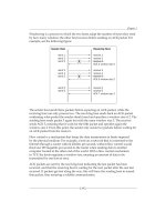
The router needs to "know" which packets are for itself, and which packets are
for which hosts with private IP addresses. The router accomplishes this by keeping
track of all TCP/IP connections that pass through it. This process is called
connection tracking.

Connection tracking gives Linux the ability to hold state information about TCP
and UDP connections in memory tables. Information about every connection is
stored in /proc/net/ip_conntrack and includes IP addresses, port numbers,
protocol types, connection state, and timeouts. Here are some example entries in
/proc/net/ip_conntrack:
tcp 6 262872 ESTABLISHED src=2.2.2.2 dst=1.1.1.1 sport=80
dport=65000 [UNREPLIED] src=192.168.1.2 dst=2.2.2.2 sport=65000
dport=80 use=1
udp 17 174 src=1.1.1.1 dst=1.1.1.11 sport=40997 dport=161
src=1.1.1.11 dst=1.1.1.1 sport=161 dport=40997 [ASSURED] use=1
Using connection tracking, the router is aware that when a packet arrives to 1.1.1.1 as
a result of a request originated from 192.168.1.2, the packet must be forwarded to the
laptop computer, and so it rewrites the destination IP address in the IP packet header
from 1.1.1.1 to 192.168.1.2.
Firewalls that do connection tracking are known as "stateful rewalls".
NAT can be performed in different scenarios:
One-to-one (1:1): We translate one private IP address into one public IP
address, for example, in the previous diagram if we perform NAT only for
the laptop computer, then we would be performing one-to-one NAT.
One-to-many (1:Many): One private IP address is translated into many public
IP addresses. This means that for each connection the private device initiates
with a host on the Internet, the NAT router chooses a public IP address from a
range to translate the private IP address into it. For example, if we performed
NAT only for the laptop computer and we have more than one public IP
address in the diagram, we would have one-to-many NAT.
Many-to-one (Many:1) This is just like in the previous diagram, where many
private IP addresses are translated into one public IP address (if the public IP
address belongs to the router, this is also known as masquerading).
Many-to-many (Many:Many): Many private IP addresses are translated using
a range of public IP addresses. If we had more than one public IP address

and we were to NAT all the computers in the earlier diagram using multiple
public IP addresses, then we would perform many-to-many NAT.
•
•
•
•
NAT and Packet Mangling with iptables
[ 92 ]
SNAT and Masquerade
SNAT is an alias for Source Network Address Translation. It is called so because only
the source IP address gets translated. The NAT box will overwrite the source address
in IP headers of all packets sent by a box behind NAT to one or many IP addresses.
One or many hosts can be translated into one or many public IP addresses only when
accessing the Internet, but when a request from the Internet is made to the public
IP address(es), the request will not reach any of the hosts (if the translated address
is the router's, it will reach the router; otherwise packets will be dropped). This is a
good protection for local networks and saves a lot of public IP addresses.
If one or many hosts behind NAT are translated into only one public IP address,
the process is called static SNAT. If they are translated into several public IP
addresses (usually a range of IP addresses), the process is called dynamic SNAT. In
the case of dynamic SNAT, the NAT router chooses an IP address from a range; so
one computer accessing the Internet is very likely to be translated into different IP
addresses for each connection it initiates. For dynamic SNAT, iptables chooses the
least used IP address from the specied range. If many IP addresses from the range
are not used at all, iptables randomly chooses one of those.
Masquerade or MASQ works exactly like static SNAT does, except that you cannot
specify the public IP address to be used. It will automatically use the IP address of
the outgoing interface of the NAT router.
SNAT was introduced with iptables, and did not exist in
netlter for kernels lower than 2.4. However, Masquerade

was kept in iptables simply because with interfaces like PPP
adapters that receive a dynamically assigned IP address, it
is simpler to do a MASQ rather than nd the dynamically
assigned IP address and do SNAT.
In order to do SNAT or Masquerade, the router needs to use connection tracking
so that it "knows" where to send ows of data belonging to connections initiated by
hosts behind NAT.
Chapter 4
[ 93 ]
The following diagram presents an example of how SNAT or Masquerade works:
In this diagram, the computer with the IP address 192.168.1.3 tries to initiate a
connection to 2.2.2.2. The packet is passed to the Linux router with the source IP
address 192.168.1.3 and destination IP address 2.2.2.2.
If the computer is SNATed or Masqueraded, the Linux router will change the source
IP address in the packet header from 192.168.1.3 to 1.1.1.1 and will pass the packet
towards 2.2.2.2 according to the routing process. Information about this connection is
stored in /proc/net/ip_conntrack.
When 2.2.2.2 replies, the IP packet that arrives in the Linux router will have
source IP address 2.2.2.2 and destination IP address 1.1.1.1. Linux searches for
information about this packet in /proc/net/ip_conntrack, and nds a match
against information stored at the previous step. At this point, Linux will change the
destination IP address in the packet header to 192.168.1.3 and will pass the IP packet
towards the NATed computer according to the routing process.
NAT and Packet Mangling with iptables
[ 94 ]
Using SNAT or Masquerade, 192.168.1.3 can initiate a
connection to 2.2.2.2, but 2.2.2.2 can't initiate a connection to
192.168.1.3, because this is a private IP address.
DNAT
DNAT or Destination Network Address Translations maps a public IP address to

a private IP address. DNAT is the reverse of SNAT; so, if you SNAT to translate a
private IP address into a public IP address and DNAT to translate the same public IP
address into the same private IP address, the result will be full NAT.
DNAT is usually used when you have servers behind NAT, so the same public IP
address is mapped to different private IP addresses depending on ports or protocols.
This process is also called port forwarding.
Let's take a look at the following diagram:
Chapter 4
[ 95 ]
Normally, 2.2.2.2 cannot initiate a communication to 192.168.1.3 because this is a
private IP address and is not routed on the Internet.
2.2.2.2 tries to initiate a connection with 1.1.1.1. If a DNAT rule is matched for this
packet, the Linux router will change the destination IP address in the IP packet
header from 1.1.1.1 to 192.168.1.3, pass the packet towards 192.168.1.3, and keep a
track of this connection.
When 192.168.1.3 replies, the packet is found in the conntrack table of the Linux
router so it "knows" that the packet belongs to the connection initiated by 2.2.2.2 to
1.1.1.1. The Linux router will change the source IP address in the IP packet header
from 192.168.1.3 to 1.1.1.1.
If DNAT is congured, but SNAT is not, 2.2.2.2 will be
able to establish connections to 192.168.1.3 using 1.1.1.1 as
destination IP address, but 192.168.1.3 will not be able to
initiate connections to 2.2.2.2.
To get a little off-topic here, there are quite a lot of SOHO routers calling their DNAT
functions DMZ. Actually, most of the SOHO routers call DNAT DMZ, which is not
entirely correct. DMZ, acronym for Demilitarized Zone is a place in your network
where you don't lter anything. DMZ is basically a set of public IP addresses that
are allowed to do anything (all incoming and outgoing trafc to and from these IP
addresses is allowed to pass without exceptions).
Due to the fact that most SOHO routers are programmed to Masquerade for a LAN,

they call a process in which one private IP address receives all (unltered) trafc
destined to the public IP of the router's WAN interface DMZ.
Full NAT (aka Full Cone NAT)
Full NAT is a way to fully map one IP address to another. With full NAT, one
device behind the NAT box which has a private IP address (e.g. 192.168.1.3) will be
seen on the Internet as another IP address routed to the NAT box by the provider
(e.g. 1.1.1.1).
This means that when a request is sent by 192.168.1.3 to any device on the Internet,
the receiving device will "see" that it received a packet from 1.1.1.1 (so far, this is
simple source NAT). More than that, for any packet from the Internet with the
destination IP address 1.1.1.1, the NAT box will rewrite the destination address in
the IP header to 192.168.1.3 and will forward that packet to 192.168.1.3, even if the
connection was not initiated by 192.168.1.3 (this is simple destination NAT).
NAT and Packet Mangling with iptables
[ 96 ]
In other words, full NAT is SNAT and DNAT as presented earlier.
This is the function that SOHO routers call "DMZ", as explained earlier. The reason
they call this function "DMZ" is that IP packets that don't belong to a connection
initiated by any host from the private network 192.168.1.0/24 will be forwarded to
192.168.1.3, and so this host doesn't have the protection provided by the fact that it
has a private IP address.
In the case just presented, 1.1.1.1 can be the NAT router
IP address or it can just be routed to it. If it's the router's
public IP address (as in the earlier diagrams),
the NAT router can't be accessed from the Internet
(e.g. you can't SSH into it) because it will forward all
packets to 192.168.1.3.
PAT or NAPT
PAT stands for Port Address Translation and it is also called NAPT, which stands for
Network Address and Port Translation. The idea behind PAT is to translate not only

the IP address, but also the port number for specic hosts and ports.
The company's web server is behind NAT and it has the IP address 192.168.1.100.
Having only one public IP address, http://www.<ourcompanyname>.com is
congured to respond to 1.1.1.1. For the web server to be accessed from the Internet,
we have to rewrite the address 1.1.1.1 to 192.168.1.100 whenever a request comes into
our NAT router with the destination port 80.
More than this, we have a company intranet server with the IP address 192.168.1.200,
running a web server on port 80. When being in the ofce, the employees have to
type http://192.168.1.200 in their web browser and they can log in the intranet
web server.
If we want to allow users to log on to the intranet server when they are outside the
ofce, PAT is the answer. With PAT, we can choose a port that's not opened on the
NAT router (e.g. 2143), and whenever a request comes from the Internet with the
destination IP address 217.156.123.3 and the destination port 2143, the NAT router
rewrites the destination IP address to 192.168.1.200 and the destination port from
2143 to 80.
This way, from the Internet when a user types:
http://www.<ourcompanyname>.com/ the request is forwarded to
192.168.1.100 on port 80 and the company's web page is displayed
•
Chapter 4
[ 97 ]
http://www.<ourcompanyname>.com:2143/ the request is forwarded to
192.168.1.200 on port 80 and the company's intranet web page is displayed
We don't have to rewrite the port when a packet has the source IP address
192.168.1.200; we just have to set up SNAT or Masquerade so that the intranet server
accesses the Internet using 1.1.1.1.
NAT Using iptables
So far, we discussed general NAT principles, NAT types, and what every sort of
NAT does.

netlter/iptables can be used to perform NAT in any of the ways that we discussed.
Actually, there are many things that you can do with iptables in this area and we will
try to cover as much as possible in this chapter. Before we get there, let's see what we
need to be able to successfully perform NAT on Linux.
Setting Up the Kernel
Usually, every Linux distribution comes with a kernel compiled with netlter
support, iptables tool, and all the modules needed for performing Network
Address Translation.
A very good HowTo on compiling Linux 2.4 and 2.6 kernels is written by
Kwan Lowe and can be found at
Kernel-Build-HOWTO.html
When compiling a new kernel or recompiling the kernel that you have, you must set
NETFILTER=y in order to use iptables. In the 2.6 kernels, this option is usually found
under Device Drivers | Networking support | Networking support (NET [=y]) |
Networking options, but it really depends on the kernel version.
For example, in kernel 2.6.14, this option is found under Networking | Networking
Options.
If you use make menuconfig or make xconfig to congure your kernel for
recompiling, select Networking | Networking options | Network packet ltering
(replaces ipchains) | IP: Netlter Conguration:
•
NAT and Packet Mangling with iptables
[ 98 ]
In the IP: Netlter Conguration section you will nd the options needed for NAT
as follows:
IP_NF_CONNTRACK or Connection tracking (required for masq/NAT) keeps
a record of the IP packets that passed through the machine in order to pass
them correctly to the NATed endpoints when requests made from those are
answered. This is vital for NAT. If you say No here, you will not be able to
perform NAT.

•
Chapter 4
[ 99 ]
It is highly recommended that you select M for conntrack,
meaning that you compile the connection tracking option
of netlter as a module. In time, you might want to use
your Linux box to do routing without NAT, and conntrack
would slow things down in that case.
IP_NF_NAT or Full NAT allows you to do SNAT, DNAT, MASQ, and
redirects. You must select this module for NAT.
IP_NF_TARGET_MASQUERADE or MASQUERADE target support is needed for
MASQ. If you will need MASQ, select this module.
IP_NF_TARGET_REDIRECT or REDIRECT target support is needed to do
redirection of packets to the local machine instead of letting them pass
through. We will need this if we want to set up a transparent proxy,
for example.
IP_NF_TARGET_NETMAP or NETMAP target support is an implementation of
static 1:1 NAT mapping of a network address.
IP_NF_TARGET_SAME or SAME target support is exactly like SNAT, except
that when using a range of public IP addresses for a network, SAME tries to
allocate clients the same IP address for all outgoing connections.
•
•
•
•
•