Advanced 3D Game Programming with DirectX - phần 8 ppsx

498

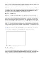
Figure 9.23: Subdividing edges to add triangles
The equation we use to subdivide an edge depends on the valence of its endpoints. The valence of a
vertex in this context is defined as the number of other vertices the vertex is adjacent to. There are three
possible cases that we have to handle.
The first case is when both vertices of a particular edge have a valence = 6. We use a mask on the
neighborhood of vertices around the edge. This mask is where the modified butterfly scheme gets its
name, because it looks sort of like a butterfly. It appears in Figure 9.24
.

Figure 9.24: The butterfly mask
The modified butterfly scheme added two points and a tension parameter that lets you control the
sharpness of the limit surface. Since this scheme complicates the code, I chose to go with a universal

499
w-value of 0.0 instead (which resolves to the above Figure 9.24
). The modified butterfly mask appears
in Figure 9.25
.

Figure 9.25: The modified butterfly mask
To compute the location of the subdivided edge vertex (the white circle in both images), we step around
the neighborhood of vertices and sum them (multiplying each vector by the weight dictated by the
mask). You'll notice that all the weights sum up to 1.0. This is good; it means our subdivided point will
be in the right neighborhood compared to the rest of the vertices. You can imagine if the sum was much
larger the subdivided vertex would be much farther away from the origin than any of the vertices used to
create it, which would be incorrect.
When only one of our vertices is regular (i.e., has a valence = 6), we compute the subdivided location
using the irregular vertex, otherwise known as a k-vertex. This is where the modified butterfly algorithm

shines over the original butterfly algorithm (which handled k-vertices very poorly). An example appears
in Figure 9.26
. The right vertex has a valence of 6, and the left vertex has a valence of 9, so we use the
left vertex to compute the location for the new vertex (indicated by the white circle).

500

Figure 9.26: Example of a k-vertex
The general case for a k-vertex has us step around the vertex, weighting the neighbors using a mask
determined by the valence of the k-vertex. Figure 9.27
shows the generic k-vertex and how we name
the vertices. Note that the k-vertex itself has a weight of ¾, in all cases.

Figure 9.27: Generic k-vertex
There are three cases to deal with: k = 3, k = 4, and k = 5. The masks for each of them are:


501
The third and final case we need to worry about is when both endpoints of the current edge are k-
vertices. When this occurs we compute the k-vertex for both endpoints using the above weights, and
average the results together.
Note that we are assuming that our input triangle mesh is closed boundary representation (doesn't have
any holes in it). The paper describing the modified butterfly scheme discusses ways to handle holes in
the model (with excellent results) but the code we'll write next won't be able to handle holes in the model
so we won't discuss it.
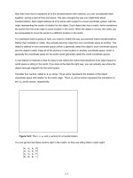
Using these schema for computing our subdivided locations results in an extremely fair looking surface.
Figure 9.28
shows how an octahedron looks as it is repeatedly subdivided. The application we will make
next was used to create this image.

Levels 0 (8 triangles) through 4 (2048 triangles) are shown. Finally, level 4 mesh is shown in filled
mode.

Figure 9.28: A subdivided octagon model.
Application: SubDiv
The SubDiv application implements the modified butterfly subdivision scheme we just discussed. It
loads an .o3d file and displays it interactively, giving the user the option of subdividing the model
whenever they wish.
The model data is represented with an adjacency graph. Each triangle structure holds pointers to the
three vertices it is composed of. Each vertex structure has STL vectors that contain pointers to edge
structures (one edge for each vertex it's connected to) and triangle structures. The lists are unsorted
(which requires linear searching; fixing this to order the edges in clockwise winding order, for example,
is left as an exercise for the reader).

502
Listing 9.8
gives the header definitions (and many of the functions) for the vertex, edge, and triangle
structures. These classes are all defined inside the subdivision surface class (cSubDivSurf).
Listing 9.8: Vertex, edge, and triangle structures

/**
* Subdivision Surface vertex (name 'sVertex' is used in D3D code)
*/
struct sVert
{
/**
* These two arrays describe the adjacency information
* for a vertex. Each vertex knows who all of its neighboring
* edges and triangles are. An important note is that these
* lists aren't sorted. We need to search through the list

* when we need to get a specific adjacent triangle.
* This is, of course, inefficient. Consider sorted insertion
* an exercise to the reader.
*/
std::vector< sTriangle* > m_triList;
std::vector< sEdge* > m_edgeList;
/**

* position/normal information for the vertex
*/
sVertex m_vert;

/**
* Each Vertex knows its position in the array it lies in.
* This helps when we're constructing the arrays of
* subdivided data.
*/
int m_index;

503

void AddEdge( sEdge* pEdge )
{
assert( 0 == std::count(
m_edgeList.begin(),
m_edgeList.end(),
pEdge ) );
m_edgeList.push_back( pEdge );
}

void AddTri( sTriangle* pTri )
{
assert( 0 == std::count(
m_triList.begin(),
m_triList.end(),
pTri ) );
m_triList.push_back( pTri );
}

/**
* Valence == How many other vertices are connected to this one
* which said another way is how many edges the vert has.
*/
int Valence()
{
return m_edgeList.size();
}

sVert() :
m_triList( 0 ),
m_edgeList( 0 )
{

504
}

/**
* Given a Vertex that we know we are attached to, this function
* searches the list of adjacent edges looking for the one that
* contains the input vertex. Asserts if there is no edge for

* that vertex.
*/
sEdge* GetEdge( sVert* pOther )
{
for( int i=0; i<m_edgeList.size(); i++ )
{
if( m_edgeList[i]->Contains( pOther ) )

return m_edgeList[i];
}
assert(false); // didn't have it!
return NULL;
}
};

/**
* Edge structure that connects two vertices in a SubSurf
*/
struct sEdge
{
sVert* m_v[2];

/**
* When we perform the subdivision calculations on all the edges
* the result is held in this newVLoc strucure. Never has any
* connectivity information, just location and color.

505
*/
sVert m_newVLoc;

/**
* true == one of the edges' vertices is the inputted vertex
*/
bool Contains( sVert* pVert )
{
return (m_v[0] == pVert) || m_v[1] == pVert;
}

/**
* retval = the other vertex than the inputted one
*/
sVert* Other( sVert* pVert )
{
return (m_v[0] == pVert) ? m_v[1] : m_v[0];
}

void Init( sVert* v0, sVert* v1 )
{
m_v[0] = v0;
m_v[1] = v1;

/**
* Note that the edge notifies both of its vertices that it's
* connected to them.
*/
m_v[0]->AddEdge( this );
m_v[1]->AddEdge( this );
}

506
/**
* This function takes into consideration the two triangles that
* share this edge. It returns the third vertex of the first
* triangle it finds that is not equal to 'notThisOne'. So if

* want one, notThisOne is passed as NULL. If we want the other
* one, we pass the result of the first execution.
*/
sVert* GetOtherVert( sVert* v0, sVert* v1, sVert* notThisOne )
{
sTriangle* pTri;
for( int i=0; i<v0->m_triList.size(); i++ )
{
pTri = v0->m_triList[i];
if( pTri->Contains( v0 ) && pTri->Contains( v1 ) )
{
if( pTri->Other( v0, v1 ) != notThisOne )
return pTri->Other( v0, v1 );
}
}
// when we support boundary edges, we shouldn't assert
assert(false);
return NULL;
}

/**
* Calculate the K-Vertex location of 'prim' vertex. For triangles
* of valence !=6

*/
point3 CalcKVert( int prim, int sec );

/**

507
* Calculate the location of the subdivided point using the
* butterfly method.
* for edges with both vertices of valence == 6
*/
point3 CalcButterfly();
};

/**
* Subdivision surface triangle
*/
struct sTriangle
{

/**
* The three vertices of this triangle
*/
sVert* m_v[3];
point3 m_normal;

void Init( sVert* v0, sVert* v1, sVert* v2 )
{
m_v[0] = v0;
m_v[1] = v1;
m_v[2] = v2;

/**
* Note that the triangle notifies all 3 of its vertices
* that it's connected to them.
*/

m_v[0]->AddTri( this );
m_v[1]->AddTri( this );

508
m_v[2]->AddTri( this );
}

/**
* true == the triangle contains the inputted vertex
*/
bool Contains( sVert* pVert )
{
return pVert == m_v[0] || pVert == m_v[1] || pVert == m_v[2];
}

/**
* retval = the third vertex (first and second are inputted).
* asserts out if inputted values aren't part of the triangle
*/
sVert* Other( sVert* v1, sVert* v2 )
{
assert( Contains( v1 ) && Contains( v2 ) );
for( int i=0; i<3; i++ )
{

if( m_v[i] != v1 && m_v[i] != v2 )
return m_v[i];
}
assert(false); // something bad happened;
return NULL;
}
};


The interesting part of the application is when the model is subdivided. Since we used vertex buffers to
hold the subdivided data, we have an upper bound of 2
16
, or 65,536, vertices. Listing 9.9 gives the code
that gets called when the user subdivides the model.

509
Listing 9.9: The code to handle subdivision

result cSubDivSurf::Subdivide()
{
/**
* We know how many components our subdivided model will have,
* calc them
*/
int nNewEdges = 2*m_nEdges + 3*m_nTris;
int nNewVerts = m_nVerts + m_nEdges;
int nNewTris = 4*m_nTris;

/**
* Find the location of the new vertices. Most of the hard work

* is done here.
*/
GenNewVertLocs();

int i;

// the vertices on the 3 edges (order: 0 1, 1 2, 2 0)
sVert* inner[3];

// Allocate space for the subdivided data
sVert* pNewVerts = new sVert[ nNewVerts ];
sEdge* pNewEdges = new sEdge[ nNewEdges ];
sTriangle* pNewTris = new sTriangle[ nNewTris ];

//==========
Step 1: Fill vertex list

// First batch - the original vertices

510
for( i=0; i<m_nVerts; i++ )
{
pNewVerts[i].m_index = i;
pNewVerts[i].m_vert = m_pVList[i].m_vert;
}
// Second batch - vertices from each edge
for( i=0; i<m_nEdges; i++ )
{
pNewVerts[m_nVerts + i].m_index = m_nVerts + i;
pNewVerts[m_nVerts + i].m_vert = m_pEList[i].m_newVLoc.m_vert;

}

//==========
Step 2: Fill edge list

int currEdge = 0;
// First batch - the 2 edges that are spawned by each original edge
for( i=0; i<m_nEdges; i++ )
{
pNewEdges[currEdge++].Init(
&pNewVerts[m_pEList[i].m_v[0]->m_index],
&pNewVerts[m_pEList[i].m_newVLoc.m_index] );
pNewEdges[currEdge++].Init(
&pNewVerts[m_pEList[i].m_v[1]->m_index],
&pNewVerts[m_pEList[i].m_newVLoc.m_index] );
}
// Second batch - the 3 inner edges spawned by each original tri
for( i=0; i<m_nTris; i++ )
{
// find the inner 3 vertices of this triangle
// ( the new vertex of each of the triangles' edges )
inner[0] = &m_pTList[i].m_v[0]->GetEdge(

511
m_pTList[i].m_v[1] )->m_newVLoc;
inner[1] = &m_pTList[i].m_v[1]->GetEdge(
m_pTList[i].m_v[2] )->m_newVLoc;
inner[2] = &m_pTList[i].m_v[2]->GetEdge(
m_pTList[i].m_v[0] )->m_newVLoc;

pNewEdges[currEdge++].Init(
&pNewVerts[inner[0]->m_index],

&pNewVerts[inner[1]->m_index] );
pNewEdges[currEdge++].Init(
&pNewVerts[inner[1]->m_index],
&pNewVerts[inner[2]->m_index] );
pNewEdges[currEdge++].Init(
&pNewVerts[inner[2]->m_index],
&pNewVerts[inner[0]->m_index] );
}

//==========
Step 3: Fill triangle list

int currTri = 0;
for( i=0; i<m_nTris; i++ )
{
// find the inner vertices
inner[0] = &m_pTList[i].m_v[0]->GetEdge(
m_pTList[i].m_v[1] )->m_newVLoc;
inner[1] = &m_pTList[i].m_v[1]->GetEdge(
m_pTList[i].m_v[2] )->m_newVLoc;
inner[2] = &m_pTList[i].m_v[2]->GetEdge(
m_pTList[i].m_v[0] )->m_newVLoc;


512
// 0, inner0, inner2
pNewTris[currTri++].Init(

&pNewVerts[m_pTList[i].m_v[0]->m_index],
&pNewVerts[inner[0]->m_index],
&pNewVerts[inner[2]->m_index] );

// 1, inner1, inner0
pNewTris[currTri++].Init(
&pNewVerts[m_pTList[i].m_v[1]->m_index],
&pNewVerts[inner[1]->m_index],
&pNewVerts[inner[0]->m_index] );

// 2, inner2, inner1
pNewTris[currTri++].Init(
&pNewVerts[m_pTList[i].m_v[2]->m_index],
&pNewVerts[inner[2]->m_index],
&pNewVerts[inner[1]->m_index] );

// inner0, inner1, inner2
pNewTris[currTri++].Init(
&pNewVerts[inner[0]->m_index],
&pNewVerts[inner[1]->m_index],
&pNewVerts[inner[2]->m_index] );
}

//==========
Step 4: Housekeeping

// Swap out the old data sets for the new ones.

delete [] m_pVList;

513
delete [] m_pEList;
delete [] m_pTList;

m_nVerts = nNewVerts;
m_nEdges = nNewEdges;
m_nTris = nNewTris;

m_pVList = pNewVerts;
m_pEList = pNewEdges;
m_pTList = pNewTris;

// Calculate the vertex normals of the new mesh
// using face normal averaging
CalcNormals();

//==========
Step 5: Make arrays so we can send the triangles in one batch

delete [] m_d3dTriList;
if( m_pVertexBuffer )
m_pVertexBuffer->Release();
m_pVertexBuffer = NULL;

GenD3DData();

return res_AllGood;
}

/**
* This is where the meat of the subdivision work is done.
* Depending on the valence of the two endpoints of each edge,
* the code will generate the new edge value

514
*/
void cSubDivSurf::GenNewVertLocs()
{
for( int i=0; i<m_nEdges; i++ )
{
int val0 = m_pEList[i].m_v[0]->Valence();
int val1 = m_pEList[i].m_v[1]->Valence();

point3 loc;

/**
* CASE 1: both vertices are of valence == 6
* Use the butterfly scheme
*/
if( val0 == 6 && val1 == 6 )
{
loc = m_pEList[i].CalcButterfly();
}

/**
* CASE 2: one of the vertices are of valence == 6
* Calculate the k-vertex for the non-6 vertex

*/

else if( val0 == 6 && val1 != 6 )
{
loc = m_pEList[i].CalcKVert(1,0);
}
else if( val0 != 6 && val1 == 6 )
{
loc = m_pEList[i].CalcKVert(0,1);
}

515

/**
* CASE 3: neither of the vertices are of valence == 6
* Calculate the k-vertex for each of them, and average
* the result
*/
else
{
loc = ( m_pEList[i].CalcKVert(1,0) +
m_pEList[i].CalcKVert(0,1) ) / 2.f;
}

m_pEList[i].m_newVLoc.m_vert = sVertex(
loc , point3::Zero );

/**
* Assign the new vertex an index (this is useful later,
* when we start throwing vertex pointers around. We
* could have implemented everything with indices, but
* the code would be much harder to read. An extra dword

* per vertex is a small price to pay.)
*/
m_pEList[i].m_newVLoc.m_index=i+ m_nVerts;
}
}

point3 cSubDivSurf::sEdge::CalcButterfly()
{
point3 out = point3::Zero;

sVert* other[2];
other[0] = GetOtherVert( m_v[0], m_v[1], NULL );

516
other[1] = GetOtherVert( m_v[0], m_v[1], other[0] );

// two main ones
out += (1.f/2.f) * m_v[0]->m_vert.loc;
out += (1.f/2.f) * m_v[1]->m_vert.loc;

// top/bottom ones
out += (1.f/8.f) * other[0]->m_vert.loc;
out += (1.f/8.f) * other[1]->m_vert.loc;

// outside 4 verts
out += (-1.f/16.f) *
GetOtherVert( other[0], m_v[0], m_v[1] )->m_vert.loc;

out += (-1.f/16.f) *
GetOtherVert( other[0], m_v[1], m_v[0] )->m_vert.loc;

out += (-1.f/16.f) *
GetOtherVert( other[1], m_v[0], m_v[1] )->m_vert.loc;
out += (-1.f/16.f) *
GetOtherVert( other[1], m_v[1], m_v[0] )->m_vert.loc;

return out;
}

point3 cSubDivSurf::sEdge::CalcKVert(int prim, int sec)
{
int valence = m_v[prim]->Valence();

point3 out = point3::Zero;

out += (3.f / 4.f) * m_v[prim]->m_vert.loc;


517
if( valence<3)
assert( false );

else if( valence == 3 )
{
for( int i=0; i<m_v[prim]->m_edgeList.size(); i++ )
{
sVert* pOther =
m_v[prim]->m_edgeList[i]->Other( m_v[prim] );
if( pOther == m_v[sec] )
out += (5.f/12.f) * pOther->m_vert.loc;
else

out += (-1.f/12.f) * pOther->m_vert.loc;
}
}

else if( valence == 4 )
{
out += (3.f/8.f) * m_v[sec]->m_vert.loc;

sVert* pTemp = GetOtherVert( m_v[0], m_v[1], NULL );
// get the one after it
sVert* pOther = GetOtherVert( m_v[prim], pTemp, m_v[sec] );

out += (-1.f/8.f) * pOther->m_vert.loc;
}

else // valence >= 5
{
sVert* pCurr = m_v[sec];
sVert* pLast = NULL;
sVert* pTemp;

518
for( int i=0; i< valence; i++ )
{
float weight =
((1.f/4.f) +
(float)cos(2*PI* (float)i / (float)valence ) +

(1.f/2.f) * (float)cos(4*PI*(float)i/(float)valence))
/ (float)valence;

out += weight * pCurr->m_vert.loc;

pTemp = GetOtherVert( m_v[prim], pCurr, pLast );
pLast = pCurr;
pCurr = pTemp;
}
}
return out;
}

void cSubDivSurf::GenD3DData()
{
/**
* Create a vertex buffer
*/
HRESULT hr;
hr = Graphics()->GetDevice()->CreateVertexBuffer(
m_nVerts * sizeof( sVertex ),
D3DUSAGE_WRITEONLY,
D3DFVF_XYZ | D3DFVF_NORMAL | D3DFVF_TEX1,
D3DPOOL_DEFAULT,
&m_pVertexBuffer );


519
if( FAILED( hr ))
{
throw cGameError("Vertex Buffer creation failed!\n");
}

m_d3dTriList = new sTri[ m_nTris ];

sVertex* pVert;

// Lock the vertex buffer
hr = m_pVertexBuffer->Lock(
0,
0,
(BYTE**)&pVert,
0);

if( FAILED( hr ))
{
throw cGameError("VB Lock failed\n");
}

int i;

// Copy data into the buffer
for( i=0; i<m_nVerts; i++ )
{
*pVert++ = m_pVList[i].m_vert;
}
m_pVertexBuffer->Unlock();

for( i=0; i<m_nTris; i++ )
{

520

m_d3dTriList[i].v[0] = m_pTList[i].m_v[0]->m_index;
m_d3dTriList[i].v[1] = m_pTList[i].m_v[1]->m_index;
m_d3dTriList[i].v[2] = m_pTList[i].m_v[2]->m_index;
}
}


Progressive Meshes
The final multiresolution system we are going to discuss is progressive meshes. They're rapidly gaining
favor in the game community; many games use them as a way to keep scene detail at a constant level.
Oftentimes when we're playing a 3D game, many of our objects will appear off in the distance. For
example, if we're building a combat flight simulator, bogies will appear miles away before we engage
them. When an object is this far away, it will appear to be only a few pixels on the screen.
We could simply opt not to draw an object if it is this far away. However, this can lead to a discontinuity
of experience for the user. He or she will suddenly remember they're playing a video game, and that
should be avoided at all costs. If we have a model with thousands of triangles in it to represent our
enemy aircraft, we're going to waste a lot of time transforming and lighting vertices when we'll end up
with just a blob of a few pixels. Drawing several incoming bogie blobs may max out our triangle budget
for the frame, and our frame rate will drop. This will hurt the user experience just as much if not more
than not drawing the object in the first place.
Even when the object is moderately close, if most of the triangles are smaller than one pixel big, we're
wasting effort on drawing our models. If we used, instead, a lower resolution version of the mesh to use
at farther distances, the visual output would be about the same, but we would save a lot of time in
model processing.
This is the problem progressive meshes try to solve. They allow us to arbitrarily scale the polygon
resolution of a mesh from its max all the way down to two triangles. When our model is extremely far
away, we draw the lowest resolution model we can. Then, as it approaches the camera, we slowly add
detail polygon by polygon, so the user always will be seeing a nearly ideal image at a much faster frame
rate. Moving between detail levels on a triangle-by-triangle basis is much less noticeable than switching
between a handful of models at different resolutions. We can even morph our triangle-by-triangle

transitions using what are called geomorphs, making them even less noticeable.
Progressive meshes can also help us when we have multiple close objects on the screen. If we used
just the distance criterion discussed above to set polygon resolution, we could easily have the case
where there are multiple dense objects close to the camera. We would have to draw them all at a high
resolution, and we would hit our polygon budget and our frame rate would drop out. In this extreme

521
situation, we can suffer some visual quality loss and turn down the polygon count of our objects. In
general, when a user is playing an intense game, he or she won't notice that the meshes are lower
resolution. Users will, however, immediately notice a frame rate reduction.
One thing progressive meshes can't do is add detail to a model. Unlike the other two multiresolution
surface methods we have discussed, progressive meshes can only vary the detail in a model from its
original polygon count down to two polygons.
Progressive meshes were originally described in a 1996 SIGGRAPH paper by Hugues Hoppe. Since
then a lot of neat things have happened with them. Hoppe has applied them to view-dependent level-of-
detail and terrain rendering. They were added to Direct3D Retained Mode (which is no longer
supported). Recently, Hoppe extended research done by Michael Garland and Paul Heckbert, using
quadric error metrics to encode normal, color, and texture information. We'll be covering some of the
basics of quadric error metrics, and Hoppe's web site has downloadable versions of all his papers. The
URL is />.
Progressive Mesh Basics
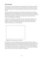
How do progressive meshes work? They center around an operation called an edge collapse.
Conceptually, it takes two vertices that share an edge and merges them. This destroys the edge that
was shared and the two triangles that shared the edge.
The cool thing about edge collapse is that it only affects a small neighborhood of vertices, edges, and
triangles. We can save the state of those entities in a way that we can reverse the effect of the edge
collapse, splitting a vertex into two, adding an edge, and adding two triangles. This operation, the
inverse of the edge collapse, is called a vertex split. Figure 9.29
shows how the edge collapse and
vertex split work.

Figure 9.29: The edge collapse and vertex split operations

522
To construct a progressive mesh, we take our initial mesh and iteratively remove edges using edge
collapses. Each time we remove an edge, the model loses two triangles. We then save the edge
collapse we performed into a stack, and continue with the new model. Eventually, we reach a point
where we can no longer remove any edges. At this point we have our lowest resolution mesh and a
stack of structures representing each edge that was collapsed. If we want to have a particular number of
triangles for our model, all we do is apply vertex splits or edge collapses to get to the required number
(plus or minus one, though, since we can only change the count by two).
During run time, most systems have three main areas of data: a stack of edge collapses, a stack of
vertex splits, and the model. To apply a vertex split, we pop one off the stack, perform the requisite
operations on the mesh, construct an edge collapse to invert the process, and push the newly created
edge collapse onto the edge collapse stack. The reverse process applies to edge collapses.
There are a lot of cool side effects that arise from progressive meshes. For starters, they can be stored
on disk efficiently. If an application is smart about how it represents vertex splits, storing the lowest
resolution mesh and the sequence of vertex splits to bring it back to the highest resolution model
doesn't take much more space than storing the high-resolution mesh on its own.
Also, the entire mesh doesn't need to be loaded all at once. A game could load the first 400 or so
triangles of each model at startup and then load more vertex splits as needed. This can save some time
if the game is being loaded from disk, and a lot of time if the game is being loaded over the Internet.
Another thing to consider is that since the edge collapses happen in such a small region, many of them
can be combined together, getting quick jumps from one resolution to another. Each edge
collapse/vertex split can even be morphed, smoothly moving the vertices together or apart. This
alleviates some of the popping effects that can occur when progressive meshes are used without any
morphing. Hoppe calls these transitions geomorphs.
Choosing Our Edges
The secret to making a good progressive mesh is choosing the right edge to collapse during each
iteration. The sequence is extremely important. If we choose our edges unwisely, our low-resolution

mesh won't look anything like our high-resolution mesh.
As an extreme example, imagine we chose our edges completely at random. This can have extremely
adverse effects on the way our model looks even after a few edge collapses.

Warning
Obviously, we should not choose vertices completely at random. We have to take
other factors into account when choosing an edge. Specifically, we have to
maintain the topology of a model. We shouldn't select edges that will cause seams
in our mesh (places where more than two triangles meet an edge).