Advanced 3D Game Programming with DirectX - phần 10 potx

640
const polygon< point3 >& in )
{
int i;
m_camLoc = camLoc;
m_nPlanes = 0;
for( i=0; i< in.nElem; i++ )
{
/**
* Plane 'i' contains the camera location and the 'ith'
* edge around the polygon
*/
m_planes[ m_nPlanes++ ] = plane3(
camLoc,
in.pList[(i+1)%in.nElem],
in.pList[i] );
}
}

bool cViewCone::Clip( const polygon<point3>& in,polygon<point3>* out )
{
/**
* Temporary polygons. This isn't thread safe
*/
static polygon<point3> a(32), b(32);
polygon<point3>* pSrc = &a;
polygon<point3>* pDest = &b;

int i;

/**
* Copy the input polygon to a.
*/

641
a.nElem = in.nElem;
for( i=0; i<a.nElem; i++ )
{
a.pList[i] = in.pList[i];
}

/**
* Iteratively clip the polygon
*/
for( i=0; i<m_nPlanes; i++ )
{
if( !m_planes[i].Clip( *pSrc, pDest ) )
{
/**
* Failure
*/
return false;
}
std::swap( pSrc, pDest );
}

/**
* If we make it here, we have a polygon that survived.
* Copy it to out.
*/

out->nElem + pSrc->nElem;
for( i=0; i<pSrc->nElem; i++ )
{
out->pList[i] = pSrc->pList[i];
}

/**

642
* Success
*/
return true;
}


You can perform portal rendering in one of two ways, depending on the fill rate of the hardware you're
running on and the speed of the host processor. The two methods are exact portal rendering and
approximative portal rendering.
Exact Portal Rendering
To render a portal scene using exact portal rendering, you use a simple recursive algorithm. Each cell
has a list of polygons, a list of portals, and a visited bit. Each portal has a pointer to the cell adjacent to
it. You start the algorithm knowing where the camera is situated, where it's pointing, and which cell it is
sitting in. From this, along with other information like the height, width, and field of view of the camera,
you can determine the initial viewing cone that represents the entire viewable area on the screen. Also,
you clear the valid bit for all the cells in the scene.
You draw all of the visible regions of the cell's polygons (the visible regions are found by clipping the
polygons against the current viewing cone). Also, you set the visited bit to true. Then you walk the list of
portals for the cell. If the cell on the other side hasn't been visited, you try to clip the portal against the
viewing cone. If a valid portal fragment results from the operation, you have the area of the portal that
was visible from the current viewing cone. Take the resulting portal fragment and use it to generate a

new viewing cone. Finally, you recurse into the cell adjacent to the portal in question using the new
viewing cone. You repeat this process until there are no new cells to traverse into. Pseudocode to do
this appears in Listing 11.3
.
Listing 11.3: Pseudocode for exact portal rendering

void DrawSceneExact
for( all cells )
cell.visited = false
currCell = cell camera is in
currCone = viewing cone of camera
currCell.visited = true
VisitCell( currCell, currCone )
void VisitCell( cell, viewCone )

643
for( each polygon in cell )
polygon fragment = viewCone.clip( current polygon )
if( polygon fragment is valid )
draw( polygon fragment )
for( each portal )
portal fragment = viewCone.clip( current portal )
if( portal fragment is valid )
if( !portal.otherCell.visited )
portal.otherCell.visited = true
newCone = viewing cone of portal fragment
VisitCell( portal.otherCell, newCone )


I haven't talked about how to handle rendering objects (such as enemies, players, ammo boxes, and so

forth) that would be sitting in these cells. It's almost impossible to guarantee zero overdraw if you have
to draw objects that are in cells. Luckily, there is the z-buffer so you don't need to worry; you just draw
the objects for a particular cell when you recurse into it. Handling objects without a depth buffer can get
hairy pretty quickly; be happy you have it.
Approximative Portal Rendering
As the fill rate of cards keeps increasing, it's becoming less and less troublesome to just throw up your
hands and draw some triangles that won't be seen. The situation is definitely much better than it was a
few years ago, when software rasterizers were so slow that you wouldn't even think of wasting time
drawing pixels you would never see. Also, since the triangle rate is increasing so rapidly it's quickly
getting to the point where the time you spend clipping off invisible regions of a triangle takes longer than
it would to just draw the triangle and let the hardware sort any problems out.
In approximative portal rendering, you only spend time clipping portals. Objects in the cells and the
triangles making up the cell boundaries are either trivially rejected or drawn. When you want to draw an
object, you test the bounding sphere against the frustum. If the sphere is completely outside the
frustum, you know that it's completely obscured by the cells you've already drawn, so you don't draw the
object. If any part of it is visible, you just draw the entire object, no questions asked. While you do spend
time drawing invisible triangles (since part of the object may be obscured) you make up for it since you
can draw the object without any special processing using one big DrawIndexedPrimitive or something
similar. The same is true for portal polygons. You can try to trivially reject polygons in the cell and save
some rendering time or just blindly draw all of them when you enter the cell.

644
Another plus when you go with an approximative portal rendering scheme is that the cells don't need to
be strictly convex; they can have any number of concavities in them and still render correctly if a z-
buffer is used. Remember, however, that things like containment tests become untrivial when you go
with concave cells; you can generally use something like a BSP tree for each cell to get around these
problems.
Portal Effects
Assuming that all of the portals and cells are in a fixed location in 3D, there isn't anything terribly
interesting that you do with portal rendering. However, that's a restriction you don't necessarily need to

put on yourself. There are a few nifty effects that can be done almost for free with a portal rendering
engine, two of which I'll cover here: mirrors and teleporters.
Mirrors
Portals can be used to create mirrors that reflect the scene back onto you. Using them is much easier
when you're using exact portal rendering (clipping all drawn polygons to the boundaries of the viewing
cone for the cell the polygons are in); when they're used with approximative portal rendering, a little
more work needs to be done.
Mirrors can be implemented with a special portal that contains a transformation matrix and a pointer
back to the parent cell. When this portal is reached, the viewing cone is transformed by the portal's
transformation matrix. You then continue the recursive portal algorithm, drawing the cell we're in again
with the new transformation matrix that will make it seem as if we are looking through a mirror.

Warning
Note that you should be careful when using multiple mirrors in a scene. If two
mirrors can see each other, it is possible to infinitely recurse between both portals
until the stack overflows. This can be avoided by keeping track of how many times
you have recursed into a mirror portal and stopping after some number of iterations.
To implement mirrors you need two pieces of information: How do you create the mirror transformation
matrix, and how do you transform the viewing cone by that matrix? I'll answer each of these questions
separately.
Before you can try to make the mirror transformation matrix, you need an intuitive understanding of what
the transformation should do. When you transform the viewing cone by the matrix, you will essentially
be flipping it over the mirror such that it is sitting in world space exactly opposite where it was before.
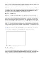
Figure 11.4
shows what is happening.

645

Figure 11.4: 2D example of view cone reflection
For comprehension's sake, let's give the mirror its own local coordinate space. To define it, you need

the n, o, a, and p vectors to put the matrix together (see Chapter 5
). The p vector is any point on the
mirror; you can just use the first vertex of the portal polygon. The a vector is the normal of the portal
polygon (so in the local coordinate space, the mirror is situated at the origin in the x-y plane). The n
vector is found by crossing a with any vector that isn't parallel to it (let's just use the up direction,
<0,1,0>) and normalizing the result. Given n and a, o is just the normalized cross product of the two.
Altogether this becomes:


Warning
The cross product is undefined when the two vectors are parallel, so if the mirror is
on the floor or ceiling you should use a different vector rather than <0,1,0>. <1,0,0>
will suffice.
However, a transformation matrix that converts points local to the mirror to world space isn't terribly
useful by itself. To actually make the mirror transformation matrix you need to do a bit more work. The
final transformation needs to perform the following steps:
 Transform world space vertices to the mirror's local coordinate space. This can be accomplished
by multiplying the vertices by T
mirror
−
1
.

646
 Flip the local space vertices over the x-y plane. This can be accomplished by using a scaling
transformation that scales by 1 in the x and y directions and −1 in the z direction (see Chapter 5
).
We'll call this transformation T
reflect
.

 Finally, transform the reflected local space vertices back to world space. This can be
accomplished by multiplying the vertices by T
mirror
.
Given these three steps you can compose the final transformation matrix, M
mirror
.

Given M
mirror
, how do you apply the transformation to the viewing cone, which is just a single point and a
set of planes? I haven't discussed how to apply transformations to planes yet, but now seems like a
great time. There is a real way to do it, given the plane defined as a 1x4 matrix:

If you don't like that, there's a slightly more intuitive way that requires you to do a tiny bit more work. The
problem with transforming normals by a transformation matrix is that you don't want them to be
translated, just rotated. If you translated them they wouldn't be normal-length anymore and wouldn't
correctly represent a normal for anything. If you just zero-out the translation component of M
mirror
, (M
14
,
M
24
, and M
34
), and multiply it by the normal component of the plane, it will be correctly transformed.
Alternatively you can just do a 1x4 times 4x4 operation, making the first vector [a,b,c,0].

Warning

This trick only works for rigid-body transforms (ones composed solely of rotations,
translations, and reflections).
So you create two transformation matrices, one for transforming regular vectors and one for
transforming normals. You multiply the view cone location by the vector transformation matrix and
multiply each of the normals in the view cone planes by the normal transformation matrix. Finally,
recompute the d components for each of the planes by taking the negative dot product of the
transformed normal and the transformed view cone location (since the location is sitting on each of the
planes in the view cone).
You should postpone rendering through a mirror portal until you have finished with all of the regular
portals. When you go to draw a mirror portal, you clone the viewing cone and transform it by M
mirror
.
Then you reset all of the visited bits and continue the algorithm in the cell that owned the portal. This is
done for all of the mirrors visited. Each time you find one, you add it to a mirror queue of mirror portals
left to process.
You must be careful if you are using approximative portal rendering and you try to use mirrors. If you
draw cells behind the portal, the polygons will interfere with each other because of z-buffer issues.

647
Technically, what you see in a mirror is a flat image, and should always occlude things it is in front of.
The way you are rendering a mirror (as a regular portal walk) it has depth, and faraway things in the
mirror may not occlude near things that should technically be behind it. To fix this, before you render
through the mirror portal, you change the z-buffer comparison function to D3DCMP_ALWAYS and draw
a screen space polygon over the portal polygon with the depth set to the maximum depth value. This
essentially resets the z-buffer of the portal region so that everything drawn through the mirror portal will
occlude anything drawn behind it. I recommend you use exact portal rendering if you want to do mirrors
or translocators, which I'll discuss next.
Translocators and Non-Euclidean Movement
One of the coolest effects you can do with portal rendering is create non-Euclidean spaces to explore.
One effect is having a doorway floating in the middle of a room that leads to a different area; you can

see the different area through the door as you move around it. Another effect is having a small structure
with a door, and upon entering the structure you realize there is much more space inside of it than could
be possible given the dimensions of the structure from the outside. Imagine a small cube with a small
door that opens into a giant amphitheater. Neither of these effects is possible in the real world, making
them all the neater to have in a game.
You perform this trick in a way similar to the way you did mirrors, with a special transformation matrix
you apply to the viewing cone when you descend through the portal. Instead of a mirror portal which
points back to the cell it belongs to, a translocator portal points to a cell that can be anywhere in the
scene. There are two portals that are the same size (but not necessarily the same orientation), a source
portal and a destination portal. When you look through the source portal, the view is seen as if you were
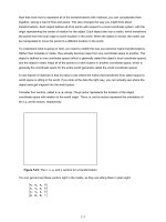
looking through the destination portal. Figure 11.5
may help explain this.

Figure 11.5: 2D representation of the translocator transformation

648
To create the transformation matrix to transform the view cone so that it appears to be looking through
the destination portal, you compute local coordinate space matrices for both portals using the same n,
o, a, and p vectors we used in the mirrors section. This gives you two matrices, T
source
and T
dest
. Then to
compute M
translocator
, you do the following steps:
 Transform the vectors from world space to the local coordinate space of the source matrix
(multiply them by T
source
−

1
).
 Take the local space vectors and transform them back into world space, but use the destination
transformation matrix(T
dest
).
Given these steps you can compose the final transformation matrix:

The rendering process for translocators is identical to rendering mirrors and has the same caveats when
approximative portal rendering is used.
Portal Generation
Portal generation, or finding the set of convex cells and interconnecting portals given an arbitrary set of
polygons, is a fairly difficult problem. The algorithm I'm going to describe is too complex to fully describe
here; it would take much more space than can be allotted. However, it should lead you in the generally
right direction if you wish to implement it. David Black originally introduced me to this algorithm.
The first step is to create a leafy BSP of the data set. Leafy BSPs are built differently than node BSPs
(the kind discussed in Chapter 5
). Instead of storing polygons and planes at the nodes, only planes are
stored. Leaves contain lists of polygons. During construction, you take the array of polygons and
attempt to find a plane from the set of polygon planes that divides the set into two non-zero sets.
Coplanar polygons are put into the side that they face, so if the normal to the polygon is the same as the
plane normal, it is considered in front of the plane. Trying to find a splitter will fail if and only if the set of
polygons forms a convex cell. If this happens, the set of polygons becomes a leaf; otherwise the plane
is used to divide the set into two pieces, and the algorithm recurses on both pieces. An example of tree
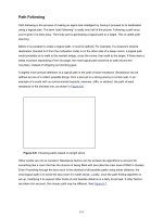
construction on a simple 12-polygon 2D data set appears in Figure 11.6
.

649

Figure 11.6: Constructing a leafy BSP tree

The leaves of the tree will become the cells of the data set, and the nodes will become the portals. To
find the portal polygon given the plane at a node, you first build a polygon that lies in the plane but
extends out in all directions past the boundaries of the data set.
This isn't hideously difficult. You keep track of a universe box, a cube that is big enough to enclose the
entire data set. You look at the plane normal to find the polygon in the universe box that is the most
parallel to it. Each of the four vertices of that universe box polygon are projected into the plane. You
then drop that polygon through the tree, clipping it against the cells that it sits in. After some careful
clipping work (you need to clip against other polygons in the same plane, polygons in adjacent cells,
etc.), you get a polygon that isn't obscured by any of the geometry polygons. This becomes a portal
polygon.
After you do this for each of the splitting planes, you have a set of cells and a set of portal polygons but
no association between them. Generating the associations between cells and portals is fairly involved,
unfortunately. The sides of a cell may be defined by planes far away, so it's difficult to match up a portal
polygon with a cell that it is abutting. Making the problem worse is the fact that some portal polygons
may be too big, spanning across several adjacent cells. In this case you would need to split the cell up.
On top of all that, once you get through this mess and are left with the set of cells and portals, you'll
almost definitely have way too many cells and way too many portals. Combining cells isn't easy. You
could just merge cells only if the new cell they formed was convex, but this will also give you a less-
than-ideal solution: you may need to merge together three or more cells together to get a nice big
convex cell, but you wouldn't be able to reach that cell if you couldn't find pairs of cells out of the set that
formed convex cells.
Because of problems like this, many engines just leave the process of portal cell generation up to the
artists. If you're using approximative portal rendering the artists can place portals fairly judiciously and
end up with concave cells, leaving them just in things like doorways between rooms and whatnot.

650
Quake II used something like this to help culling scenes behind closed doors; area portals would be
covering doors and scenes behind them would only be traversed if the doors weren't closed.
Precalculated Portal Rendering (PVS)
Up to this point I have discussed the usage of portal rendering to find the set of visible cells from a

certain point in space. This way you can dynamically find the exact set of visible cells you can see from
a certain viewpoint. However, you shouldn't forget one of the fundamental optimization concepts in
computer programming: Why generate something dynamically if you can precalculate it?
How do you precalculate the set of visible cells from a given viewpoint? The scene has a near infinite
number of possible viewpoints, and calculating the set of visible cells for each of them would be a
nightmare. If you want to be able to precalculate anything, you need to cut down the space of entries or
cut down the number of positions for which you need to precalculate.
What if you just considered each cell as a whole? If you found the set of all the cells that were visible
from any point in the cell, you could just save that. Each of the n cells would have a bit vector with n
entries. If bit i in the bit vector is true, then cell i is visible from the current cell.
This technique of precalculating the set of visible cells for each cell was pioneered by Seth Teller in his
1992 thesis. The data associated with each cell is called the Potentially Visible Set, or PVS for short. It
has since been used in Quake, Quake II, and just about every other first-person shooter under the sun.
Doing this, of course, forces you to give up exact visibility. The set of visible cells from all points inside a
cell will almost definitely be more than the set of visible cells from one particular point inside the cell, so
you may end up drawing some cells that are totally obscured from the camera. However, what you lose
in fill-rate, you gain in processing time. You don't need to do any expensive frustum generation or cell
traversal; you simply step through the bit vector of the particular cell and draw all the cells whose bits
are set.
Advantages/Disadvantages
The big reason this system is a win is because it offloads work from the processor to the hardware.
True, you'll end up drawing more polygons than you have to, but it won't be that much more. The extra
cost in triangle processing and fill rate is more than made up for since you don't need to do any frustum
generation or polygon clipping.
However, using this system forces you to give up some freedom. The time it takes to compute the PVS
is fairly substantial, due to the complexity of the algorithm. This prevents you from having your cells
move around; they must remain static. This, however, is forgivable in most cases; the geometry that
defines walls and floors shouldn't be moving around anyway.
Implementation Details

651
I can't possibly hope to cover the material required to implement PVS rendering; Seth Teller spends 150
pages doing it in his thesis. However, I can give a sweeping overview of the pieces of code involved.
The first step is to generate a cell and portal data set, using something like the algorithm discussed
earlier. It's especially important to keep your cell count down, since you have an n
2
memory cost to hold
the PVS data (where n is the number of cells). Because of this, most systems use the concept of detail
polygons when computing the cells. Detail polygons are things like torches or computer terminals—
things that don't really define the structural boundaries of a scene but just introduce concavities. Those
polygons generally are not considered until the PVS table is calculated. Then they are just added to the
cells they belong to. This causes the cells to be concave, but the visibility information will still remain the
same, so we're all good.
Once you have the set of portals and cells, you iteratively step through each cell and find the set of
visible cells from it. To do this, you do something similar to the frustum generation we did earlier in the
chapter, but instead of a viewing cone coming out of a point, you generate a solid that represents what
is viewable from all points inside the solid. An algorithm to do this (called portal stabbing) is given in
Seth Teller's thesis. Also, the source code to QV (the application that performs this operation for the
Quake engine) is available online.
When finished, and you have the PVS vector for each of the cells, rendering is easy. You can easily find
out which cell the viewer is in (since each of the cells is convex). Given that cell, you step through the bit
vector for that cell. If bit i is set, you draw cell i and let the z-buffer sort it out.
Application: Mobots Attack!
The intent of Mobots Attack! was to make an extremely simple client-server game that would provide a
starting point for your own 3D game project. As such, it is severely lacking in some areas but fairly
functional in others. There is only one level and it was crafted entirely by hand. Physics support is
extremely lacking, as is the user interface. However, it has a fairly robust networking model that allows
players to connect to a server, wander about, and shoot rockets at each other.
The objective of the game wasn't to make something glitzy. It doesn't use radiosity, AI opponents,
multitexture, or any of the multi-resolution modeling techniques we discussed in Chapter 9

. However,
adding any of these things wouldn't be terribly difficult. Hopefully, adding cool features to an existing
project will prove more fruitful for you than trying to write the entire project yourself. Making a project
that was easy to add to was the goal of this game. I'll quickly cover some of the concepts that make this
project work.
Interobject Communication
One of the biggest problems in getting a project of this size to work in any sort of reasonable way is
interobject communication. For example, when an object hits a wall, some amount of communication
needs to go on between the object and the wall so that the object stops moving. When a rocket hits an

652
object, the rocket needs to inform the object that it must lose some of its hit points. When a piece of
code wants to print debugging info, it needs to tell the application object to handle it.
Things get even worse. When the client moves, it needs some way to tell the server that its object has
moved. But how would it do that? It's not like it can just dereference a pointer and change the position
manually; the server could be in a completely different continent.
To take care of this, a messaging system for objects to communicate with each other was implemented.
Every object that wanted to communicate needed to implement an interface called iGameObject, the
definition of which appears in Listing 11.4
:
Listing 11.4: The iGameObject interface

typedef uint msgRet;

interface iGameObject
{
public:
virtual objID GetID() = 0;
virtual void SetID( objID id)=0;
virtual msgRet ProcMsg( const sMsg& msg)=0;

};


An objID is an int masquerading as two shorts. The high short defines the class of object that the ID
corresponds to, and the low short is the individual instance of that object. Each object in the game has a
different objID, and that ID is the same across all the machines playing a game (the server and each of
the clients). The code that runs the objID appears in Listing 11.5
.
Listing 11.5: objID code

typedef uint objID;

inline objID MakeID( ushort segment, ushort offset )
{
return (((uint)segment)<<16) | ((uint)offset);

653
}

inline ushort GetIDSegment( objID id )
{
return (ushort)(id>>16);
}

inline ushort GetIDOffset( objID id )
{
return (ushort)(id & 0xFFFF);
}

/**

* These segments define the types of objects
*/
const ushort c_sysSegment = 0; // System object
const ushort c_cellSegment = 1; // Cell object
const ushort c_playerSegment = 2; // Player object
const ushort c_spawnSegment = 3; // Spawning object
const ushort c_projSegment = 4; // Projectile object
const ushort c_paraSegment = 5; // Parametric object
const ushort c_tempSegment = 6; // Temp object


All object communication is done by passing messages around. In the same way you would send a
message to a window to have it change its screen position in Windows, you send a message to an
object to have it perform a certain task. The message structure holds onto the destination object (an
objID), the type of the message (which is a member of the eMsgType enumeration), and then some
extra data that has a different meaning for each of the messages. The sMsg structure appears in Listing
11.6.
Listing 11.6: Pseudocode for exact portal rendering


654
struct sMsg
{
eMsgType m_type;
objID m_dest;
union
{
struct
{
point3 m_pt;

};
struct
{
plane3 m_plane;
};
struct
{
color3 m_col;
};
struct
{
int m_i[4];
};
struct
{
float m_f[4];
};
struct
{
void* m_pData;
};
};


655
sMsg( eMsgType type = msgForceDword, objID dest=0)
: m_type( type )
, m_dest( dest )
{
}

sMsg( eMsgType type, objID dest, float f )
: m_type( type )
, m_dest( dest )
{
m_f[0] = f;
}
sMsg( eMsgType type, objID dest, int i )
: m_type( type )
, m_dest( dest )
{
m_i[0] = i;
}
sMsg( eMsgType type, objID dest, const point3& pt )
: m_type( type )
, m_dest( dest )
, m_pt(pt)
{
}
sMsg( eMsgType type, objID dest, const plane3& plane )
: m_type( type )
, m_dest( dest )
, m_plane(plane)
{
}
sMsg( eMsgType type, objID dest, void* pData )
: m_type( type )

656
, m_dest( dest )

, m_pData( pData )
{
}
};


When an object is created, it registers itself with a singleton object called the message daemon
(cMsgDaemon). The registering process simply adds an entry into a map that associates a particular ID
with a pointer to an object. Typically what happens is when an object is created, a message will be
broadcast to the other connected machines telling them to make the object as well and providing it with
the ID to use in the object creation. The cMsgDaemon class appears in Listing 11.7
.
Listing 11.7: Code for the message daemon

class cMsgDaemon
{
map< objID, iGameObject* >m_objectMap;
static cMsgDaemon* m_pGlobalMsgDaemon;

public:
cMsgDaemon();
~cMsgDaemon();

static cMsgDaemon* GetMsgDaemon()
{
// Accessor to the singleton
if( !m_pGlobalMsgDaemon )
{
m_pG1oba1MsgDaemon = new cMsgDaemon
}

return m_pGlobalMsgDaemon;
}

657

void RegObject( objID id, iGameObject* pObj );
void UnRegObject( objID id );

iGameObject* Get( int id )
{
return m_objectMap[id];
}

/**
* Deliver this message to the destination
* marked in msg.m_dest. Throws an exception
* if no such object exists.
*/
uint DeliverMessage( const sMsg& msg );
};


When one object wants to send a message to another object, it just needs to fill out an sMsg structure
and then call cMsgDaemon::DeliverMessage (or a nicer-looking wrapper use function SendMessage).
In some areas of code, rather than ferry a slew of messages back and forth, a local-scope pointer to an
object corresponding to an ID can be acquired with cMsgDaemon::Get and then member functions can
be called.
Network Communication
The networking model this game has is remarkably simple. There is no client-side prediction and no
extrapolation. While this makes for choppy gameplay, hopefully it should make it easier to understand.

The messaging model I implemented here was strongly based on an article written by Mason McCuskey
for GameDev.net called "Why pluggable factories rock my multiplayer world."
Here's the essential problem pluggable factories try to solve. Messages arrive to you as datagrams,
essentially just buffers full of bits. Those bits represent a message that was sent to you from another
client. The first byte (or short, if there are a whole lot of messages) is an ID tag that describes what the
message is (a tag of 0x07, for example, may be the tag for a message describing the new position of an
object that moved). Using the ID tag, you can figure out what the rest of the data is.

658
How do you figure out what the rest of the data is? One way would be to just have a massive switch
statement with a case label for each message tag that will take the rest of the data and construct a
useful message. While that would work, it isn't the right thing to do, OOP-wise. Higher-level code (that
is, the code that constructs the network messages) needs to know details about lower-level code (that
is, each of the message IDs and to what each of them correspond).
Pluggable factories allow you to get around this. Each message has a class that describes it. Every
message derives from a common base class called cNetMessage, which appears in Listing 11.8
.
Listing 11.8: Code for the cNetMessage class

/**
* Generic Message
* Every message class derives from this one.
*/
class cNetMessage
{
public:
cNetMessage()
{
}
-cNetMessage()

{
}

/**
* Write out a bitstream to be sent over the wire
* that encapsulates the data of the message.
*/
virtual int SerializeTo( uchar* pOutput )
{
return 0;
}


659
/**
* Take a bitstream as input (coming in over
* the wire) and convert it into a message
*/
virtual void SerializeFrom( uchar *pFromData, int datasize )
{
}

/**
* This is called on a newly constructed message.
* The message in essence executes itself. This
* works because of the objID system; the message
* object can communicate its desired changes to
* the other objects in the system.
*/
virtual void Exec() = 0;

netID GetFrom()
{
return m_from;
}
netID GetTo()
{
return m_to;
}

void SetFrom( netID id )
{
m_from = id;
}

void SetTo( netID id )

660
{
m_to = id;
}

protected:
netID m_from;
netID m_to;
};


Every derived NetMessage class has a sister class that is the maker for that particular class type. For
example, the login request message class cNM_LoginRequest has a sister maker class called

cNM_LoginRequestMaker. The maker class's responsibility is to create instances of its class type. The
maker registers itself with a map in the maker parent class. The map associates those first-byte IDs with
a pointer to a maker object. When a message comes off the wire, a piece of code looks up the ID in the
map, gets the maker pointer, and tells the maker to create a message object. The maker creates a new
instance of its sister net message class, calls Serialize-From on it with the incoming data, and returns
the instance of the class.
Once a message is created, its Exec() method is called. This is where the message does any work it
needs to do. For example, when the cNM_LoginRequest is executed (this happens on the server when
a client attempts to connect), the message tells the server (using the interobject messaging system
discussed previously) to create the player with the given name that was supplied. This will in turn create
new messages, like an acknowledgment message notifying the client that it has logged in.
Code Structure
There are six projects in the game workspace. Three of them you've seen before: math3D, netLib, and
gameLib. The other three are gameServer, gameClient, and gameCommon. I made gameCommon just
to ease the compile times; it has all the code that is common to both the client and the server.
The server is a Win32 dialog app. It doesn't link any of the DirectX headers in, so it should be able to
run on any machine with a network card. All of the render code is pretty much divorced from everything
else and put into the client library. The gameClient derives from cApplication just like every other
sample app in the book.
The downloadable files contain documentation to help you get the game up and running on your
machine; the client can connect to the local host, so a server and a client can both run on the same
machine.

661
Closing Thoughts
I've covered a lot of ground in this book. Hopefully, it has all been lucid and the steps taken haven't
been too big. If you've made it to this point, you should have enough knowledge to be able to implement
a fairly complex game.
More importantly, you hopefully have acquired enough knowledge about 3D graphics and game
programming that learning new things will come easily. Once you make it over the big hump, you start

to see all the fundamental concepts that interconnect just about all of the driving concepts and
algorithms.
Good luck with all of your endeavors.
Appendix: An STL Primer
Overview
The world has two kinds of people in it. People who love the STL and use it every day, and people who
have never learned the STL. If you're one of the latter, this appendix will hopefully help you get started.
The Standard Template Library is a set of classes and functions that help coders use basic containers
(like linked lists and dynamic arrays) and basic algorithms (like sorting). It was officially introduced into
the C++ library by the ANSI/ISO C++ Standards Committee in July 1994. Almost all C++ compilers (and
all of the popular ones) implement the STL fairly well, while some implementations are better than
others (the SGI implementation is one of the better ones; it does a few things much more efficiently than
the Visual C++ implementation).
Almost all of the classes in the STL are template classes. This makes them usable with any type of
object or class, and they are also compiled entirely as inline, making them extremely fast.
Templates
A quick explanation of templates: They allow you to define a generic piece of code that will work with
any type of data, be it ints, floats, or classes.
The canonical example is Swap. Normally, if you want to swap integers in one place and swap floats in
another, you write something like Listing A.1
.
Listing A.1: Non-template code

void SwapInt( int &a, int &b )
{
int temp = a;

662
a = b;
b = temp;

}

void SwapFloat( float &a, float &b )
{
float temp = a;
a = b;
b = temp;
}


This is tolerable as long as you're only swapping around these two types, but what if you start swapping
other things? You would end up with 10 or 15 different Swap functions in some file. The worst part is
they're all exactly the same, except for the three tokens that declare the type. Let's make Swap a
template function. Its source is in Listing A.2
.
Listing A.2: Template code

template < class swapType >
void Swap( swapType &a, swapType &b )
{
swapType temp = a;
a = b;
b = temp;
}


Here's how it works. You use the templated Swap function like you would any other. When the compiler
encounters a place that you use the function, it checks the types that you're using, and makes sure
they're valid (both the same, since you use T for both a and b). Then it makes a custom piece of code
specifically for the two types you're using and compiles it inline. A way to think of it is the compiler does

a find-replace, switching all instances of swapType (or whatever you name your template types; most
people use T) to the types of the two variables you pass into swap. Because of this, the only penalty for

663
using templates is during compilation; using them at run time is just as fast as using custom functions.
There's also a small penalty since using everything inline can increase your code size. However for a
large part this point is moot—most STL functions are short enough that the code actually ends up being
smaller. Inlining the code for small functions takes less space than saving/restoring the stack frame.
Of course, even writing your own templated Swap() function is kind of dumb, as the STL library has its
own function (swap())… but it serves as a good example. Templated classes are syntactically a little
different, but we'll get to those in a moment.
Containers
STL implements a set of basic containers to simplify most programming tasks; I used them everywhere
in the text. While there are several more, Table A.1
lists the most popular ones.


Table A.1: The basic container classes
vector Dynamic array class. You append entries on the end (using push_back()) and then can
access them using standard array notation (via an overloaded [] operator). When the array
needs more space, it internally allocates a bigger block of memory, copies the data over
(explicitly, not bitwise), and releases the old one. Inserting data anywhere but the back is
slow, as all the other entries need to be moved back one slot in memory.

deque DeQueue class. Essentially a dynamic array of dynamic arrays. The data doesn't sit linear
in memory, but you can get array-style lookups really quickly, and can append to the front
or the back quickly.

list Doubly linked list class. Inserting and removing anywhere is cheap, but you can't randomly
access things; you can only iterate forward or backard.

slist Singly linked list class. Inserting to the front is quick, to the back is extremely slow. You
shouldn't need to use this since list is sufficiently fast for most code that would be using a
linked list anyway.

map This is used in a few places in the code; it is an associative container that lets you look up
entries given a key. An example would be telephone numbers. You would make a map
like so:
map<string, int> numMap;

664
and be able to say things like:
numMap["joe"] = 5553298;

stack A simple stack class.

queue A simple queue class.

string A vector of characters, with a lot of useful string operations implemented.

Let's look at some sample code. Listing A.3 creates a vector template class of integers, adds some
elements, and then asserts both.
Listing A.3: Template sample code

#include <list>
#include <vector>
#include <string>

using namespace std;

void main()
{
// Create a vector and add some numbers
vector<int> intVec;
intVec.push_back(5);
intVec.push_back(10);
assert( intVec[0] == 5 );
assert( intVec.size() == 2);
}