Advanced Control Engineering - Chapter 5 pps

//SYS21/D:/B&H3B2/ACE/REVISES(08-08-01)/ACEC05.3D ± 110 ± [110±144/35] 9.8.2001 2:30PM
5
Classical design in the
s-plane
5.1 Stability of dynamic systems
The response of a linear system to a stimulus has two components:
(a) steady-state terms which are directly related to the input
(b) transient terms which are either exponential, or oscillatory with an envelope of
exponential form.
If the exponential terms decay as time increases, then the system is said to be stable.If
the exponential terms increase with increasing time, the system is considered unstable.
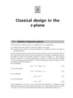
Examples of stable and unstable systems are shown in Figure 5.1. The motions
shown in Figure 5.1 are given graphically in Figure 5.2. (Note that (b) in Figure
5.2 does not represent (b) in Figure 5.1.) The time responses shown in Figure 5.2 can
be expressed mathematically as:
For (a) (Stable)
x
o
(t)  Ae
Àt
sin(!t  )(5:1)
For (b) (Unstable)
x
o
(t)  Ae
t
sin(!t  )(5:2)
For (c) (Stable)
x
o
(t)  Ae

Àt
(5:3)
For (d) (Unstable)
x
o
(t)  Ae
t
(5:4)
From equations (5.1)±(5.4), it can be seen that the stability of a dynamic system
depends upon the sign of the exponential index in the time response function, which
is in fact a real root of the characteristic equation as explained in section 5.1.1.
//SYS21/D:/B&H3B2/ACE/REVISES(08-08-01)/ACEC05.3D ± 111 ± [110±144/35] 9.8.2001 2:30PM
mg
xt
o
()
N
(c) Stable
(b) Unstable
xt
o
()
(d) Unstable
mg
N
xt
o
()
(a) Stable
xt

o
()
Fig. 5.1 Stable and unstable systems.
A
A
A
t
A
(a)
t
t
t
(b)
(c)
(d)
xt
()
o
xt
()
o
xt
()
o
xt
()
o
Fig. 5.2 Graphical representation of stable and unstable time responses.
Classical design in the s-plane 111
//SYS21/D:/B&H3B2/ACE/REVISES(08-08-01)/ACEC05.3D ± 112 ± [110±144/35] 9.8.2001 2:30PM

5.1.1 Stability and roots of the characteristic equation
The characteristic equation was defined in section 3.6.2 for a second-order system as
as
2
 bs c  0(5:5)
The roots of the characteristic equation given in equation (5.5) were shown in section
3.6.2. to be
s
1
, s
2

Àb Æ

b
2
À 4ac
p
2a
(5:6)
These roots determine the transient response of the system and for a second-order
system can be written as
(a) Overdamping
s
1
À
1
s
2
À

2
(5:7)
(b) Critical damping
s
1
 s
2
À (5:8)
(c) Underdamping
s
1
, s
2
À Æ j! (5:9)
If the coefficient b in equation (5.5) were to be negative, then the roots would be
s
1
, s
2
 Æ j! (5:10)
The roots given in equation (5.9) provide a stable response of the form given in
Figure 5.2(a) and equation (5.1), whereas the roots in equation (5.10) give an
unstable response as represented by Figure 5.2(b) and equation (5.2).
The only difference between the roots given in equation (5.9) and those in equation
(5.10) is the sign of the real part. If the real part  is negative then the system is stable,
but if it is positive, the system will be unstable. This holds true for systems of any
order, so in general it can be stated: `If any of the roots of the characteristic equation
have positive real parts, then the system will be unstable'.
5.2 The Routh±Hurwitz stability criterion
The work of Routh (1905) and Hurwitz (1875) gives a method of indicating the

presence and number of unstable roots, but not their value. Consider the character-
istic equation
a
n
s
n
 a
nÀ1
s
nÀ1
ÁÁÁa
1
s a
0
 0(5:11)
112 Advanced Control Engineering
//SYS21/D:/B&H3B2/ACE/REVISES(08-08-01)/ACEC05.3D ± 113 ± [110±144/35] 9.8.2001 2:30PM
The Routh±Hurwitz stability criterion states:
(a) For there to be no roots with positive real parts then there is a necessary, but not
sufficient, condition that all coefficients in the characteristic equation have the
same sign and that none are zero.
If (a) above is satisfied, then the necessary and sufficient condition for stability is either
(b) all the Hurwitz determinants of the polynomial are positive, or alternatively
(c) all coefficients of the first column of Routh's array have the same sign. The
number of sign changes indicate the number of unstable roots.
The Hurwitz determinants are
D
1
 a
1

D
2

a
1
a
3
a
0
a
2








D
3

a
1
a
3
a
5
a
0

a
2
a
4
a
1
a
3














D
4

a
1
a
3
a

5
a
7
a
0
a
2
a
4
a
6
a
1
a
3
a
5
a
2
a
4























etc:
(5:12)
Routh's array can be written in the form shown in Figure 5.3.
In Routh's array Figure 5.3
b
1

1
a
nÀ1
a
nÀ1
a
nÀ3
a
n
a

nÀ2








b
2

1
a
nÀ1
a
nÀ1
a
nÀ5
a
n
a
nÀ4









etc: (5:13)
c
1

1
b
1
b
1
b
2
a
nÀ1
a
nÀ3








c
2

1
b
1

b
1
b
3
a
nÀ1
a
nÀ5








etc: (5:14)
Routh's method is easy to apply and is usually used in preference to the Hurwitz
technique. Note that the array can also be expressed in the reverse order, commen-
cing with row s
n
.
·
·
q
1
p
1
·
·

s
0
s
1
s
n
–3
s
n
s
n
–2
s
n
–1
c
1
b
1
a
n
–1
a
n
c
2
b
2
a
n

–3
a
n
–2
c
3
b
3
a
n
–5
a
n
–4
··
Fig. 5.3 Routh's array.
Classical design in the s-plane 113
//SYS21/D:/B&H3B2/ACE/REVISES(08-08-01)/ACEC05.3D ± 114 ± [110±144/35] 9.8.2001 2:30PM
Example 5.1 (See also Appendix 1, A1.5)
Check the stability of the system which has the following characteristic equation
s
4
 2s
3
 s
2
 4s 2  0(5:15)
Test 1: All coefficients are present and have the same sign. Proceed to Test 2, i.e.
Routh's array
s

0
2
s
1
8
s
2
À12
s
3
24
s
4
112
(5:16)
The bottom two rows of the array in (5.16) are obtained from the characteristic
equation. The remaining coefficients are given by
b
1

1
2
24
11










1
2
(2 À 4) À1(5:17)
b
2

1
2
20
12









1
2
(4 À 0)  2(5:18)
b
3
 0(5:19)
c
1

À1
À12
24








À1(À4 À 4)  8(5:20)
c
2
 0(5:21)
d
1

1
8
80
À12










1
8
(16 À 0)  2(5:22)
In the array given in (5.16) there are two sign changes in the column therefore there
are two roots with positive real parts. Hence the system is unstable.
5.2.1 Maximum value of the open-loop gain constant for the
stability of a closed-loop system
The closed-loop transfer function for a control system is given by equation (4.4)
C
R
(s) 
G(s)
1  G(s)H(s)
(5:23)
In general, the characteristic equation is most easily formed by equating the denomi-
nator of the transfer function to zero. Hence, from equation (5.23), the characteristic
equation for a closed-loop control system is
1  G(s)H(s)  0(5:24)
114 Advanced Control Engineering
//SYS21/D:/B&H3B2/ACE/REVISES(08-08-01)/ACEC05.3D ± 115 ± [110±144/35] 9.8.2001 2:30PM
Example 5.2 (See also Appendix 1, examp52.m)
Find the value of the proportional controller gain K
1
to make the control system
shown in Figure 5.4 just unstable.
Solution
The open-loop transfer function is
G(s)H(s) 
8K

1
s(s
2
 s 2)
(5:25)
The open-loop gain constant is
K  8K
1
(5:26)
giving
G(s)H(s) 
K
s(s
2
 s 2)
(5:27)
From equation (5.24) the characteristic equation is
1 
K
s(s
2
 s 2)
 0(5:28)
or
s(s
2
 s 2)  K  0(5:29)
which can be expressed as
s
3

 s
2
 2s K  0(5:30)
The characteristic equation can also be found from the closed-loop transfer function.
Using equation (4.4)
C
R
(s) 
G(s)
1  G(s)H(s)
Given the open-loop transfer function in equation (5.27), where H(s) is unity, then
C
R
(s) 
K
s(s
2
s2)
1 
K
s(s
2
s2)
(5:31)
Cs
()
Rs
()
Plant
Control

Valve
Proportional
Controller
+
–
K
1
4
s
2
(++2)
ss
2
Fig. 5.4 Closed-loop control system.
Classical design in the s-plane 115
//SYS21/D:/B&H3B2/ACE/REVISES(08-08-01)/ACEC05.3D ± 116 ± [110±144/35] 9.8.2001 2:30PM
Multiplying numerator and denominator by s(s
2
 s 2)
C
R
(s) 
K
s(s
2
 s 2)  K
(5:32)
C
R
(s) 

K
s
3
 s
2
 2s K
(5:33)
Equating the denominator of the closed-loop transfer function to zero
s
3
 s
2
 2s K  0(5:34)
Equations (5.30) and (5.34) are identical, and both are the characteristic equation. It
will be noted that all terms are present and have the same sign (Routh's first
condition). Proceeding straight to Routh's array
s
0
K
s
1
(2 À K)
s
2
1 K
s
3
12
(5:35)
where

b
1
 1
1 K
12








 (2 À K)
b
2
 0
c
1
 K
To produce a sign change in the first column,
K ! 2(5:36)
Hence, from equation (5.26), to make the system just unstable
K
1
 0:25
Inserting (5.36) into (5.30) gives
s
3
 s

2
 2s 2  0
factorizing gives
(s
2
 2)(s 1)  0
hence the roots of the characteristic equation are
s À1
s  0 Æj

2
p
and the transient response is
c(t)  Ae
Àt
 B sin(

2t
p
 )(5:37)
From equation (5.37) it can be seen that when the proportional controller gain K
1
is
set to 0.25, the system will oscillate continuously at a frequency of

2
p
rad/s.
116 Advanced Control Engineering
//SYS21/D:/B&H3B2/ACE/REVISES(08-08-01)/ACEC05.3D ± 117 ± [110±144/35] 9.8.2001 2:30PM

5.2.2 Special cases of the Routh array
Case 1: A zero in the first column
If there is a zero in the first column, then further calculation cannot normally proceed
since it will involve dividing by zero. The problem is solved by replacing the zero with
a small number " which can be assumed to be either positive or negative. When the
array is complete, the signs of the elements in the first column are evaluated by
allowing " to approach zero.
Example 5.3
s
4
 2s
3
 2s
2
 4s 3  0
s
0
3
s
1
4 À 6/"
s
2
" 3
s
3
24
s
4
123

(5:38)
Irrespective of whether " is a small positive or negative number in array (5.38), there
will be two sign changes in the first column.
Case 2: All elements in a row are zero
If all the elements of a particular row are zero, then they are replaced by the
derivatives of an auxiliary polynomial, formed from the elements of the previous row.
Example 5.4
s
5
 2s
4
 6s
3
 12s
2
 8s 16  0
s
0
16
s
1
8/3
s
2
616
s
3
824
s
4

21216
s
5
168
(5:39)
The elements of the s
3
row are zero in array (5.39). An auxiliary polynomial P(s)is
therefore formed from the elements of the previous row (s
4
).
i.e.
P(s)  2s
4
 12s
2
 16
dP(s)
ds
 8s
3
 24s (5:40)
The coefficients of equation (5.40) become the elements of the s
3
row, allowing the
array to be completed.
Classical design in the s-plane 117
//SYS21/D:/B&H3B2/ACE/REVISES(08-08-01)/ACEC05.3D ± 118 ± [110±144/35] 9.8.2001 2:30PM
5.3 Root-locus analysis
5.3.1 System poles and zeros

The closed-loop transfer function for any feedback control system may be written in
the factored form given in equation (5.41)
C
R
(s) 
G(s)
1  G(s)H(s)

K
c
(s À z
c1
)(s À z
c2
) FFF(s Àz
cn
)
(s À p
c1
)(s À p
c2
) FFF(s Àp
cn
)
(5:41)
where s  p
c1
, p
c2
, FFF, p

cn
are closed-loop poles, so called since their values make
equation (5.41) infinite (Note that they are also the roots of the characteristic
equation) and s  z
c1
, z
c2
, FFF, z
cn
are closed-loop zeros, since their values make
equation (5.41) zero.
The position of the closed-loop poles in the s-plane determine the nature of the
transient behaviour of the system as can be seen in Figure 5.5. Also, the open-loop
transfer function may be expressed as
G(s)H(s) 
K(s À z
01
)(s À z
02
) FFF(s Àz
0n
)
(s À p
01
)(s À p
02
) FFF(s Àp
0n
)
(5:42)

where z
01
, z
02
, FFF, z
0n
are open-loop zeros and p
01
, p
02
, FFF, p
0n
are open-loop poles.
X
X
X
X
X
X
X
X
XXX
σ
X
X
X
X
jω
Fig. 5.5 Effect of closed-loop pole position in the s-plane on system transient response.
118 Advanced Control Engineering

//SYS21/D:/B&H3B2/ACE/REVISES(08-08-01)/ACEC05.3D ± 119 ± [110±144/35] 9.8.2001 2:30PM
5.3.2 The root locus method
This is a control system design technique developed by W.R. Evans (1948) that
determines the roots of the characteristic equation (closed-loop poles) when the
open-loop gain-constant K is increased from zero to infinity.
The locus of the roots, or closed-loop poles are plotted in the s-plane. This is a
complex plane, since s   Æj!. It is important to remember that the real part  is
the index in the exponential term of the time response, and if positive will make the
system unstable. Hence, any locus in the right-hand side of the plane represents an
unstable system. The imaginary part ! is the frequency of transient oscillation.
When a locus crosses the imaginary axis,   0. This is the condition of marginal
stability, i.e. the control system is on the verge of instability, where transient oscilla-
tions neither increase, nor decay, but remain at a constant value.
The design method requires the closed-loop poles to be plotted in the s-plane as K
is varied from zero to infinity, and then a value of K selected to provide the necessary
transient response as required by the performance specification. The loci always
commence at open-loop poles (denoted by x) and terminate at open-loop zeros
(denoted by o) when they exist.
Example 5.5
Construct the root-locus diagram for the first-order control system shown in
Figure 5.6.
Solution
Open-loop transfer function
G(s)H(s) 
K
Ts
(5:43)
Open-loop poles
s  0
Open-loop zeros: none

Characteristic equation
1  G(s)H(s)  0
Substituting equation (5.3) gives
1 
K
Ts
 0
i.e. Ts  K  0(5:44)
Rs
()
Cs
()
K
Ts
+
–
Fig. 5.6 First-order control system.
Classical design in the s-plane 119
//SYS21/D:/B&H3B2/ACE/REVISES(08-08-01)/ACEC05.3D ± 120 ± [110±144/35] 9.8.2001 2:30PM
Roots of characteristic equation
s À
K
T
(5:45)
When K is varied from zero to infinity the locus commences at the open-loop pole
s  0 and terminates at minus infinity on the real axis as shown in Figure 5.7.
From Figure 5.7 it can be seen that the system becomes more responsive as K is
increased. In practice, there is an upper limit for K as signals and control elements
saturate.
Example 5.6

Construct the root-locus diagram for the second-order control system shown in
Figure 5.8.
Open-loop transfer function
G(s)H(s) 
K
s(s  4)
(5:46)
Open-loop poles
s  0, À4
Open-loop zeros: none
Characteristic equation
1  G(s)H(s)  0
–∞
X
σ
jω
Fig. 5.7 Root-locus diagram for a first-order system.
Rs
()
Cs
()
K
ss
( + 4)
+
–
Fig. 5.8 Second-order control system.
120 Advanced Control Engineering
//SYS21/D:/B&H3B2/ACE/REVISES(08-08-01)/ACEC05.3D ± 121 ± [110±144/35] 9.8.2001 2:30PM
Substituting equation (5.4) gives

1 
K
s(s  4)
 0
i.e. s
2
 4s K  0(5:47)
Table 5.1 shows how equation (5.7) can be used to calculate the roots of the
characteristic equation for different values of K. Figure 5.9 shows the corresponding
root-locus diagram.
In Figure 5.9, note that the loci commences at the open-loop poles (s  0, À4)
when K  0. At K  4 they branch into the complex space. This is called a break-
away point and corresponds to critical damping.
Table 5.1 Roots of second-order characteristic
equation for different values of K
K Characteristic equation Roots
0 s
2
 4s  0 s  0, À4
4 s
2
 4s  4  0 s À2 Æ j0
8 s
2
 4s  8  0 s À2 Æ j2
16 s
2
 4s  16  0 s À2 Æ j3:46
jω
σ

3
2
1
K
=8
K
=16
K
=4
K
=8
K
=16
K
=0
X
X
K
=0
–5 –4 –3 –2 –1
–3
–1
–2
Fig. 5.9 Root locus diagram for a second-order system.
Classical design in the s-plane 121
//SYS21/D:/B&H3B2/ACE/REVISES(08-08-01)/ACEC05.3D ± 122 ± [110±144/35] 9.8.2001 2:30PM
5.3.3 General case for an underdamped second-order system
For the generalized second-order transfer function given in equation (3.43), equating
the denominator to zero gives the characteristic equation
s

2
 2!
n
s !
2
n
 0(5:48)
If <1 in equation (5.48), then the roots of the characteristic equation are
s
1
, s
2
À!
n
Æ j!
n

1 À 
2
p
(5:49)
Hence a point P in the s-plane can be represented by Figure 5.10.
From Figure 5.10, Radius
OP 

(À!
n
)
2
 !

n

1 À
2
p

2
r
(5:50)
Simplifying (5.50) gives
OP  !
n
(5:51)
Also from Figure 5.10
cos  
À!
n
jj
!
n
  (5:52)
Thus, as  is varied from zero to one, point P describes an arc of a circle of radius !
n
,
commencing on the imaginary axis (  90

) and finishing on the real axis (  0

).
Limits for acceptable transient response in the s-plane

If a system is
(1) to be stable
(2) to have acceptable transient response ( ! 0:5)
O
P
β
σ
–ζω
n
ω
n
1 –ζ
2
jω
Fig. 5.10 Roots of the characteristic equation for a second-order system shown in the s-plane.
122 Advanced Control Engineering
//SYS21/D:/B&H3B2/ACE/REVISES(08-08-01)/ACEC05.3D ± 123 ± [110±144/35] 9.8.2001 2:30PM
then the closed-loop poles must lie in an area defined by
 Æcos
À1
0:5 Æ60

(5:53)
This is illustrated in Figure 5.11.
5.3.4 Rules for root locus construction
Angle and magnitude criteria
The characteristic equation for a closed-loop system (5.24) may also be written as
G(s)H(s) À1(5:54)
Since equation (5.54) is a vector quantity, it can be represented in terms of angle and
magnitude as

=
G(s)H(s)  180

(5:55)
G(s)H(s)
jj
 1(5:56)
The angle criterion
Equation (5.55) may be interpreted as `For a point s
1
to lie on the locus, the sum of
all angles for vectors between open-loop poles (positive angles) and zeros (negative
angles) to point s
1
must equal 180

.'
In general, this statement can be expressed as
Æ Pole Angles À Æ Zero Angles  180

(5:57)
σ
60°
–60°
Acceptable
Region ( 0.5)
ζ ≥
Unacceptable
Region
j

ω
Fig. 5.11 Region of acceptable transient response in the s-plane for  !0.5.
Classical design in the s-plane 123
//SYS21/D:/B&H3B2/ACE/REVISES(08-08-01)/ACEC05.3D ± 124 ± [110±144/35] 9.8.2001 2:30PM
Example 5.7
Consider an open-loop transfer function
G(s)H(s) 
K(s  a)
s(s  b)(s c)
Figure 5.12 shows vectors from open-loop poles and zeros to a trial point s
1
. From
Figure 5.12 and equation (5.57), for s
1
to lie on a locus, then
(
1
 
2
 
3
) À(
1
)  180

(5:58)
The magnitude criterion
If a point s
1
lies on a locus, then the value of the open-loop gain constant K at that

point may be evaluated by using the magnitude criterion.
Equation (5.56) can be expressed as
jKj
jN(s)j
jD(s)j
&'
 1(5:59)
or
jKj
jD(s)j
jN(s)j
(5:60)
Equation (5.60) may be written as
K 
Product of pole vector magnitudes
Product of zero vector magnitudes
(5:61)
–ve
+ve
σ
OX X X
s
= –a
s
= –c
s
= –b
s
= 0
θ

1
θ
2
θ
3
φ
1
s
1
jω
Fig. 5.12 Application of the angle criterion.
124 Advanced Control Engineering
//SYS21/D:/B&H3B2/ACE/REVISES(08-08-01)/ACEC05.3D ± 125 ± [110±144/35] 9.8.2001 2:30PM
For Example 5.7, if s
1
lies on a locus, then the pole and zero magnitudes are shown in
Figure 5.13. From Figure 5.13 and equation (5.61), the value of the open-loop gain
constant K at position s
1
is
K 
jxjjyjjzj
jwj
(5:62)
If there are no open-loop zeros in the transfer function, then the denominator of
equation (5.62) is unity.
5.3.5 Root locus construction rules
1. Starting points (K  0): The root loci start at the open-loop poles.
2. Termination points (K I): The root loci terminate at the open-loop zeros when
they exist, otherwise at infinity.

3. Number of distinct root loci: This is equal to the order of the characteristic equation.
4. Symmetry of root loci: The root loci are symmetrical about the real axis.
5. Root locus asymptotes: For large values of k the root loci are asymptotic to
straight lines, with angles given by
 
(1  2k)
(n À m)
where
k  0, 1, FFF(n À m À 1)
n  no. of finite open-loop poles
m  no. of finite open-loop zeros
|
w
|
||
z
||
y
||
x
σ
O
XXX
s
= –a
s
= –c
s
= –b
s

= 0
s
1
jω
Fig. 5.13 Application of the magnitude criterion.
Classical design in the s-plane 125
//SYS21/D:/B&H3B2/ACE/REVISES(08-08-01)/ACEC05.3D ± 126 ± [110±144/35] 9.8.2001 2:30PM
6. Asymptote intersection: The asymptotes intersect the real axis at a point given by

a

Æ open-loop poles À Æ open-loop zeros
(n À m)
7. Root locus locations on real axis: A point on the real axis is part of the loci if the sum
of the number of open-loop poles and zeros to the right of the point concerned is odd.
8. Breakaway points: The points at which a locus breaks away from the real axis can
be calculated using one of two methods:
(a) Find the roots of the equation
dK
ds




s
b
 0
where K has been made the subject of the characteristic equation i.e. K  FFF
(b) Solving the relationship


n
1
1
(
b
jp
i
j)


m
1
1
(
b
jz
i
j)
where jp
i
j and jz
i
j are the absolute values of open-loop poles and zeros and

b
is the breakaway point.
9. Imaginary axis crossover: The location on the imaginary axis of the loci (mar-
ginal stability) can be calculated using either:
(a) The Routh±Hurwitz stability criterion.
(b) Replacing s by j! in the characteristic equation (since   0 on the imagin-

ary axis).
10. Angles of departure and arrival: Computed using the angle criterion, by position-
ing a trial point at a complex open-loop pole (departure) or zero (arrival).
11. Determination of points on root loci: Exact points on root loci are found using the
angle criterion.
12. Determination of K on root loci: The value of K on root loci is found using the
magnitude criterion.
Example 5.8 (See also Appendix 1, examp58.m and examp58a.m)
A control system has the following open-loop transfer function
G(s)H(s) 
K
s(s  2)(s 5)
(a) Sketch the root locus diagram by obtaining asymptotes, breakaway point and
imaginary axis crossover point. What is the value of K for marginal stability?
(b) Locate a point on the locus that corresponds to a closed-loop damping ratio of
0.5. What is the value of K for this condition? What are the roots of the
characteristic equation (closed-loop poles) for this value of K?
126 Advanced Control Engineering
//SYS21/D:/B&H3B2/ACE/REVISES(08-08-01)/ACEC05.3D ± 127 ± [110±144/35] 9.8.2001 2:30PM
Solution
Part (a)
Open loop poles: s  0, À2, À5 n  3
Open-loop zeros: none m  0
Asymptote angles (Rule 5)

1

(1 0)
3 À 0



3
 60

, k  0(5:63)

2

(1 2)
3 À 0
   180

, k  1(5:64)

3

(1  4)
3 À 0

5
3
 300

(À60

), k  2, i:e: n À m À1(5:65)
Asymptote intersection (Rule 6)

a


f(0)  (À2) (À5)gÀ0
3 À 0
(5:66)

a
À2:33 (5:67)
Characteristic equation: From equation (5.24)
1 
K
s(s  2)(s 5)
 0(5:68)
or
s(s  2)(s 5)  K  0
giving
s
3
 7s
2
 10s K  0(5:69)
Breakaway points (Rule 8)
Method (a): Re-arrange the characteristic equation (5.69) to make K the subject
K Às
3
À 7s
2
À 10s (5:70)
dK
ds
À3s
2

À 14s À10  0(5:71)
Multiplying through by ±1
3s
2
 14s 10  0(5:72)
s
1
, s
2
 
b

À14 Æ

14
2
À 120
p
6

b
À3:79, À0:884 (5:73)
Classical design in the s-plane 127
//SYS21/D:/B&H3B2/ACE/REVISES(08-08-01)/ACEC05.3D ± 128 ± [110±144/35] 9.8.2001 2:30PM
Method (b)
1

b

1


b
 2

1

b
 5
 0(5:74)
Multiplying through by,

b
(
b
 2)(
b
 5)
(
b
 2)(
b
 5) 
b
(
b
 5) 
b
(
b
 2)  0


2
b
 7
b
 10 
2
b
 5
b
 
2
b
 2
b
 0
3
2
b
 14
b
 10  0
(5:75)

b
À3:79, À 0:884 (5:76)
Note that equations (5.72) and (5.75) are identical, and therefore give the same roots.
The first root, À3:79 lies at a point where there are an even number of open-loop poles to
the right, and therefore is not valid. The second root, À0:884 has odd open-loop poles to
the right, and is valid. In general, method (a) requires less computation than method (b).

Imaginary axis crossover (Rule 9)
Method (a) (Routh±Hurwitz)
s
0
K
s
1
(70 À K)/7
s
2
7 K
s
3
110
From Routh's array, marginal stability occurs at K  70.
Method (b): Substitute s  j! into characteristic equation. From characteristic
equation (5.69)
(j!)
3
 7(j!)
2
 10(j!) K  0
À j!
3
À 7!
2
 10j!  K  0(5:77)
Equating imaginary parts gives
À!
3

 10!  0
!
2
 10
! Æ3:16 rad/s (5:78)
Equating real parts gives
À7!
2
 K  0
8Y K  7!
2
 70 (5:79)
Note that method (b) provides both the crossover value (i.e. the frequency of
oscillation at marginal stability) and the open-loop gain constant.
128 Advanced Control Engineering
//SYS21/D:/B&H3B2/ACE/REVISES(08-08-01)/ACEC05.3D ± 129 ± [110±144/35] 9.8.2001 2:30PM
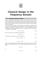
The root locus diagram is shown in Figure 5.14.
Part (b) From equation (5.52), line of constant damping ratio is
  cos
À1
()  cos
À1
(0:5)  60

(5:80)
This line is plotted on Figure 5.14 and trial points along it tested using the angle
criterion, i.e.

1
 

2
 
3
 180

At s À0:7 j1:25 (5:81)
120  44 16  180

(5:82)
Hence point lies on the locus.
Value of open-loop gain constant K: Applying the magnitude criterion to the above
point
K jajjbjjcj
 1:4 Â1:8 Â 4:5  11:35 (5:83)
4
3
2
1
0
–1
–2
–3
–9
–4
–8 –7
–6 –5
–4
–3 –2 –1
01
GsH s

() J()=
K
ss s
( +2)( +5)
ζ= 0.5
( = 60 )
β °
θ
3
θ
2
σ
a
θ
1
K
=70
K
= 11.35
Real Axis
Imaginary Axis
|b|
|a|
|c|
Fig. 5.14 Sketch of root-locus diagram for Example 5.8.
Classical design in the s-plane 129
//SYS21/D:/B&H3B2/ACE/REVISES(08-08-01)/ACEC05.3D ± 130 ± [110±144/35] 9.8.2001 2:30PM
Closed-loop poles (For K  11:35): Since the closed-loop system is third-order, there
are three closed-loop poles. Two of them are given in equation (5.81). The third lies
on the real locus that extends from À5toÀI. Its value is calculated using the

magnitude criterion as shown in Figure 5.15.
From Figure 5.15
x(x  2)(x 5)  11:35 (5:84)
Substituting x  0:73 (i.e. s
1
À5:73) in equation (5.84) provides a solution. Hence
the closed-loop poles for K  11:35 are
s À5:73, À0:7 Æ j1:25 (5:85)
Example 5.9 (See also Appendix 1, examp59.m)
The open-loop transfer function for a control system is
G(s)H(s) 
K
s(s
2
 4s 13)
Find the asymptotes and angles of departure and hence sketch the root locus
diagram. Locate a point on the complex locus that corresponds to a damping ratio
of 0.25 and hence find
(a) the value of K at this point
(b) the value of K for marginal stability
Solution
Open-loop poles: s  0,
À4 Æ

16 À 52
p
2
À2 Æ j3 n  3
Open-loop zeros: None m  0
σ

x
+ 5
x
+ 2
x
X
X
s
1
–5 –2
j
ω
Fig. 5.15 Determination of real closed-loop pole.
130 Advanced Control Engineering
//SYS21/D:/B&H3B2/ACE/REVISES(08-08-01)/ACEC05.3D ± 131 ± [110±144/35] 9.8.2001 2:30PM
Asymptote angles (Rule 5)

1

(1 0)
3 À 0


3
 60

, k  0(5:86)

2


(1 2)
3 À 0
   180

, k  1(5:87)

3

(1 4)
3 À 0

5
3
 300

, k  2, n À m À1(5:88)
Asymptote intersection (Rule 6)

a

f(0)  (À2 j3)  (À2 À j3)gÀ0
3
(5:89)

a
À1:333 (5:90)
Characteristic equation
s
3
 4s

2
 13s K  0(5:91)
Breakaway points: None, due to complex open-loop poles.
Imaginary axis crossover (Rule 9)
Method (b)
(j!)
3
 4(j!)
2
 13j! K  0
or
Àj!
3
À 4!
2
 13j!  K  0(5:92)
Equating imaginary parts
À!
3
 13!  0
!
2
 13
! Æ3:6 rad/s (5:93)
Equating real parts
À4!
2
 K  0
K  52 (5:94)
Angle of departure (Rule 10): If angle of departure is 

d
, then from Figure 5.16

a
 
b
 
d
 180


d
 180 À
a
À 
b

d
 180 À123 À90 À33

(5:95)
Locate point that corresponds to   0:25. From equation (5.52)
  cos
À1
(0:25)  75: 5

(5:96)
Classical design in the s-plane 131
//SYS21/D:/B&H3B2/ACE/REVISES(08-08-01)/ACEC05.3D ± 132 ± [110±144/35] 9.8.2001 2:30PM
Plot line of constant damping ratio on Figure 5.16 and test trial points along it using

angle criterion.
At s À0:8  j2:9
104:5  79:5 À4  180

Hence point lies on locus.
Applying magnitude criterion
K  3:0 Â6:0 Â1:25  22:5(5:97)
5.4 Design in the s-plane
The root locus method provides a very powerful tool for control system design. The
objective is to shape the loci so that closed-loop poles can be placed in the s-plane at
positions that produce a transient response that meets a given performance specifica-
tion. It should be noted that a root locus diagram does not provide information
relating to steady-state response, so that steady-state errors may go undetected,
unless checked by other means, i.e. time response.
4
3
2
1
0
–1
–2
–3
–4
–9 –8 –7
–6 –5
–4
–2
–1
01
–3

GsHs
() ()=
K
ss s
( +4 +13)
2
θ
d
θ
a
ζ= 0.25
K
= 22.5
K
=52
β
σ
a
θ
b
Real Axis
Imaginary Axis
Fig. 5.16 Root locus diagram for Example 5.9.
132 Advanced Control Engineering
//SYS21/D:/B&H3B2/ACE/REVISES(08-08-01)/ACEC05.3D ± 133 ± [110±144/35] 9.8.2001 2:30PM
5.4.1 Compensator design
A compensator, or controller, placed in the forward path of a control system will
modify the shape of the loci if it contains additional poles and zeros. Characteristics
of conventional compensators are given in Table 5.2.
In compensator design, hand calculation is cumbersome, and a suitable computer

package, such as MATLAB is generally used.
Case Study
Example 5.10 (See also Appendix 1, examp510.m)
A control system has the open-loop transfer function given in Example 5.8, i.e.
G(s)H(s) 
1
s(s  2)(s  5)
, K  1
A PD compensator of the form
G(s)  K
1
(s  a)(5:98)
is to be introduced in the forward path to achieve a performance specification
Overshoot less than 5%
Settling time (Æ2%) less than 2 seconds
Determine the values of K
1
and a to meet the specification.
Original controller
The original controller may be considered to be a proportional controller of gain K and the
root locus diagram is shown in Figure 5.14. The selected value of K  11:35 is for a
damping ratio of 0.5 which has an overshoot of 16.3% in the time domain and is not
acceptable. With adamping ratio of 0.7the overshoot is 4.6%which is within specification.
This corresponds to a controller gain of 7.13. The resulting time response for the original
system (K=11.35) is shown in Figure 5.20 where the settling time can be seen to be 5.4
seconds, which is outside of the specification. This also applies to the condition K=7.13.
PD compensator design
With the PD compensator of the form given in equation (5.98), the control problem,
with reference, to Figure 5.14, is where to place the zero a on the real axis. Potential
locations include:

(i)ii Between the poles s  0, À2, i.e. at s À1
(ii)i At s À2 (pole/zero cancellation)
(iii) Between the poles s À2, À5, i.e at s À3
Table 5.2 Compensator characteristics
Compensator Characteristics
PD One additional zero
PI One additional zero
One additional pole at origin
PID Two additional zeros
One additional pole at origin
Classical design in the s-plane 133
//SYS21/D:/B&H3B2/ACE/REVISES(08-08-01)/ACEC05.3D ± 134 ± [110±144/35] 9.8.2001 2:30PM
Option 1 (zero positioned at s À1): The cascaded compensator and plant transfer
function become
G(s)H(s) 
K
1
(s  1)
s(s  2)(s 5)
(5:99)
The root locus diagram is shown in Figure 5.17.
It can be seen in Figure 5.17 that the pole at the origin and the zero at s À1
dominate the response. With the complex loci,   0:7 gives K
1
a value of 15.
However, this value of K
1
occurs at À0:74 on the dominant real locus. The time
response shown in Figure 5.20 shows the dominant first-order response with the
oscillatory second-order response superimposed. The settling time is 3.9 seconds,

which is outside of the specification.
Option 2: (zero positioned at s À2): The cascaded compensator and plant transfer
function is
G(s)H(s) 
K
1
(s  2)
s(s  2)(s 5)
(5:100)
The root locus diagram is shown in Figure 5.18. The pole/zero cancellation may be
considered as a locus that starts at s À2 and finishes at s À2, i.e. a point on
the diagram. The remaining loci breakaway at s À2:49 and look similar to the
second-order system shown in Figure 5.9. The compensator gain K
1
that corresponds
to   0:7 is 12.8. The resulting time response is shown in Figure 5.20 and has an
overshoot of 4.1% and a settling time of 1.7 seconds, which is within specification.
4
3
2
1
0
–1
–2
–3
–4
–9 –8 –7
–6 –5
–4
–2

–1
01
–3
Imaginary Axis
Real Axis
GsHs
() ()=
Ks
1
(+1)
ss s
( + 2)( + 5)
ζ= 0.7
K
1
=15
K
1
=15
σ
a
Fig. 5.17 Root locus diagram for compensator K
1
(s  1).
134 Advanced Control Engineering