Control Systems - Part 7 pot

Appendicies

Appendix 1: Physical Models
Appendix 2: Z-Transform Mappings
Appendix 3: Transforms
Appendix 4: System Representations
Appendix 5: MatLab
Pa
g
e 164 of 209Control S
y
stems/Print version - Wikibooks, collection of o
p
en-content textbooks
10/30/2006htt
p
://en.wikibooks.or
g
/w/index.
p
h
p
?title=Control
_
S
y
stems/Print
_
version&
p

rintable=
y
es
Appendix: Physical Models
Physical Models
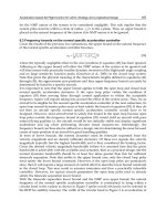
This page will serve as a refresher for various different engineering disciplines on how physical devices are
modeled. Models will be displayed in both time-domain and Laplace-domain input/output characteristics. The
only information that is going to be displayed here will be the ones that are contributed by knowledgable
contributors.
Electrical Systems
Mechanical Systems
Civil/Construction Systems
Chemical Systems

Pa
g
e 165 of 209Control S
y
stems/Print version - Wikibooks, collection of o
p
en-content textbooks
10/30/2006htt
p
://en.wikibooks.or
g
/w/index.
p
h
p
?title=Control

_
S
y
stems/Print
_
version&
p
rintable=
y
es
Appendix: Z Transform Mappings
Z Transform Mappings
There are a number of different mappings that can be used to convert a system from the complex Laplace domain
into the Z-Domain. None of these mappings are perfect, and every mapping requires a specific starting condition,
and focuses on a specific aspect to reproduce faithfully. One such mapping that has already been discussed is the
bilinear transform
, which, along with prewarping, can faithfully map the various regions in the s-plane into the
corresponding regions in the z-plane. We will discuss some other potential mappings in this chapter, and we will
discuss the pros and cons of each.
Bilinear Transform
The Bilinear transform converts from the Z-domain to the complex W domain. The W domain is not the same as
the Laplace domain, although there are some similarities. Here are some of the similiarities between the Laplace
domain and the W domain:
1. Stable poles are in the Left-Half Plane
2. Unstable poles are in the right-half plane
3. Marginally stable poles are on the vertical, imaginary axis
With that said, the bilinear transform can be defined as follows:

Graphically, we can show that the bilinear transform operates as follows:
[Bilinear Transform]
[Inverse Bilinear Transform]
Pa
g
e 166 of 209Control S
y
stems/Print version - Wikibooks, collection of o
p
en-content textbooks
10/30/2006htt
p
://en.wikibooks.or
g
/w/index.
p
h
p
?title=Control
_
S
y
stems/Print
_
version&
p
rintable=

y
es
Prewarping
The W domain is not the same as the Laplace domain, but if we employ the process of
prewarping
before we
take the bilinear transform, we can make our results match more closely to the desired Laplace Domain
representation.
Using prewarping, we can show the effect of the bilinear transform graphically:
Matched Z-Transform


Pa
g
e 167 of 209Control S
y
stems/Print version - Wikibooks, collection of o
p
en-content textbooks
10/30/2006htt
p
://en.wikibooks.or
g
/w/index.
p
h
p
?title=Control
_
S

y
stems/Print
_
version&
p
rintable=
y
es
If we have a function in the laplace domain that has been decomposed using partial fraction expansion, we
generally have an equation in the form:


And once we are in this form, we can make a direct conversion between the s and z planes using the following
mapping:



Pro
A good direct mapping in terms of s and a single coefficient
Con
requires the Laplace-domain function be decomposed using partial fraction expansion.
Simpson's Rule



CON
Essentially multiplies the order of the transfer function by a factor of 2. This makes things difficult when
you are trying to physically implement the system.
(w, v) Transform
Given the following system:

Then:




And:

[Matched Z Transform]
[Simpson's Rule]
[(w, v) Transform]
Pa
g
e 168 of 209Control S
y
stems/Print version - Wikibooks, collection of o
p
en-content textbooks
10/30/2006htt
p
://en.wikibooks.or
g
/w/index.
p
h
p
?title=Control
_
S

y
stems/Print
_
version&
p
rintable=
y
es


Pro
Directly maps a function in terms of z and s, into a function in terms of only z.
Con
Requires a function that is already in terms of s, z and α.
Z-Forms

Pa
g
e 169 of 209Control S
y
stems/Print version - Wikibooks, collection of o
p
en-content textbooks
10/30/2006htt
p
://en.wikibooks.or
g
/w/index.
p
h

p
?title=Control
_
S
y
stems/Print
_
version&
p
rintable=
y
es
Appendix: Transforms
Laplace Transform
The when we talk about the Laplace transform, we are actually talking about the version of the Laplace transform
known as the
unilinear Laplace Transform
. The other version, the
Bilinear Laplace Transform
(not related to
the Bilinear Transorm, below) is not used in this book.
The Laplace Transform is defined as:



And the Inverse Laplace Transform is defined as:



Table of Laplace Transforms

This is a table of common laplace transforms.
[Laplace Transform]
[Inverse Laplace Transform]
Time Domain Laplace Domain
Pa
g
e 170 of 209Control S
y
stems/Print version - Wikibooks, collection of o
p
en-content textbooks
10/30/2006htt
p
://en.wikibooks.or
g
/w/index.
p
h
p
?title=Control
_
S
y
stems/Print
_
version&
p
rintable=
y
es

Properties of the Laplace Transform
This is a table of the most important properties of the laplace transform.
Property Definition
Linearity
Differentiation



Frequency Division

Pa
g
e 171 of 209Control S
y
stems/Print version - Wikibooks, collection of o
p
en-content textbooks
10/30/2006htt
p
://en.wikibooks.or
g
/w/index.
p
h
p
?title=Control
_
S
y
stems/Print

_
version&
p
rintable=
y
es
Where:







Convergence of the Laplace Integral
Properties of the Laplace Transform
Fourier Transform
The Fourier Transform is used to break a time-domain signal into it's frequency domain components. The Fourier
Transform is very closely related to the Laplace Transform, and is only used in place of the Laplace transform
when the system is being analyzed in a frequency context.
The Fourier Transform is defined as:


Frequency Integration
Time Integration
Scaling
Initial value theorem
Final value theorem
Frequency Shifts

Time Shifts


Convolution Theorem
Pa
g
e 172 of 209Control S
y
stems/Print version - Wikibooks, collection of o
p
en-content textbooks
10/30/2006htt
p
://en.wikibooks.or
g
/w/index.
p
h
p
?title=Control
_
S
y
stems/Print
_
version&
p
rintable=
y

es


And the Inverse Fourier Transform is defined as:



Table of Fourier Transforms
This is a table of common fourier transforms.
[Fourier Transform]
[Inverse Fourier Transform]
Time Domain Fourier Domain
Pa
g
e 173 of 209Control S
y
stems/Print version - Wikibooks, collection of o
p
en-content textbooks
10/30/2006htt
p
://en.wikibooks.or
g
/w/index.
p
h
p
?title=Control
_
S

y
stems/Print
_
version&
p
rintable=
y
es
Note:
; is the rectangular pulse function of width

Table of Fourier Transform Properties
This is a table of common properties of the fourier transform.
Signal
Fourier transform
unitary, angular frequency
Fourier transform
unitary, ordinary
frequency
Remarks






1 Linearity
2
Shift in time
domain

3
Shift in
frequency
domain, dual of
2
4
If is large,
then is
concentrated
around 0 and

spreads out and
flattens
5
Duality
property of the
Fourier
transform.
Results from
swapping
"dummy"
variables of
and .
6
Generalized
derivative
property of the
Fourier
transform
Pa

g
e 174 of 209Control S
y
stems/Print version - Wikibooks, collection of o
p
en-content textbooks
10/30/2006htt
p
://en.wikibooks.or
g
/w/index.
p
h
p
?title=Control
_
S
y
stems/Print
_
version&
p
rintable=
y
es
Convergence of the Fourier Integral
Properties of the Fourier Transform
Z-Transform
The Z-transform is used primarily to convert discrete data sets into a continuous representation. The Z-transform
is notationally very similar to the star transform, except that the Z transform does not take explicit account for the

sampling period. The Z transform has a number of uses in the field of digital signal processing, and the study of
discrete signals in general, and is useful because Z-transform results are extensively tabulated, whereas star-
transform results are not.
The Z Transform is defined as:



Inverse Z Transform
The inverse Z Transform is a highly complex transformation, and might be inaccessible to students without
enough background in calculus. However, students who are familiar with such integrals are encouraged to
p
erform some inverse Z transform calculations, to verify that the formula produces the tabulated results.



Z-Transform Tables
7
This is the dual
to 6
8

denotes the
convolution of
and —
this rule is the
convolution
theorem
9
This is the dual
of 8

[Z Transform]
[Inverse Z Transform]
Signal, Z-transform, ROC
Pa
g
e 175 of 209Control S
y
stems/Print version - Wikibooks, collection of o
p
en-content textbooks
10/30/2006htt
p
://en.wikibooks.or
g
/w/index.
p
h
p
?title=Control
_
S
y
stems/Print
_
version&
p
rintable=
y
es
Modified Z-Transform

The Modified Z-Transform is similar to the Z-transform, except that the modified version allows for the system to
be subjected to any arbitrary delay, by design. The Modified Z-Transform is very useful when talking about
digital systems for which the processing time of the system is not negligible. For instance, a slow computer
system can be modeled as being an instantaneous system with an output delay.
The modified Z transform is based off the delayed Z transform:



Star Transform
1
2
3
4
5
6
7
8
9
10
11
[Modified Z Transform]
Pa
g
e 176 of 209Control S
y
stems/Print version - Wikibooks, collection of o
p
en-content textbooks
10/30/2006htt
p

://en.wikibooks.or
g
/w/index.
p
h
p
?title=Control
_
S
y
stems/Print
_
version&
p
rintable=
y
es
The Star Transform is a discrete transform that has similarities between the Z transform and the Laplace
Transform. In fact, the Star Transform can be said to be nearly analogous to the Z transform, except that the Star
transform explicitly accounts for the sampling time of the sampler.
The Star Transform is defined as:



Star transform pairs can be obtained by plugging into the Z-transform pairs, above.

Bilinear Transform
The bilinear transform is used to convert an equation in the Z domain into the arbitrary W domain, with the
following properties:
1. roots inside the unit circle in the Z-domain will be mapped to roots on the left-half of the W plane.

2. roots outside the unit circle in the Z-domain will be mapped to roots on the right-half of the W plane
3. roots on the unit circle in the Z-domain will be mapped onto the vertical axis in the W domain.
The bilinear transform can therefore be used to convert a Z-domain equation into a form that can be analyzed
using the Routh-Hurwitz criteria. However, it is important to note that the W-domain is not the same as the
complex Laplace S-domain. To make the output of the bilinear transform equal to the S-domain, the signal must
be prewarped, to account for the non-linear nature of the bilinear transform.
The Bilinear transform can also be used to convert an S-domain system into the Z domain. Again, the input
system must be prewarped prior to applying the bilinear transform, or else the results will not be correct.
The Bilinear transform is governed by the folloing variable transformations:



Where T is the sampling time of the discrete signal.
Frequencies in the w domain are related to frequencies in the s domain through the following relationship:


This relationship is called the
frequency warping characteristic
of the bilinear transform. To counter-act the
effects of frequency warping, we can
pre-warp
the Z-domain equation using the inverse warping charateristic. If
the equation is prewarped before it is transformed, the resulting poles of the system will line up more faithfully
with those in the s-domain.
[Star Transform]
[Bilinear Transform]
Pa
g
e 177 of 209Control S
y

stems/Print version - Wikibooks, collection of o
p
en-content textbooks
10/30/2006htt
p
://en.wikibooks.or
g
/w/index.
p
h
p
?title=Control
_
S
y
stems/Print
_
version&
p
rintable=
y
es



Applying these transformations before applying the bilinear transform actually enables direct conversions
between the S-Domain and the Z-Domain. The act of applying one of these frequency warping characteristics to a
function before transforming is called
prewarping
.

Wikipedia Resources

w:Laplace transform

w:Fourier transform

w:Z-transform

w:Star transform

w:Bilinear transform

[Bilinear Frequency Prewarping]
Pa
g
e 178 of 209Control S
y
stems/Print version - Wikibooks, collection of o
p
en-content textbooks
10/30/2006htt
p
://en.wikibooks.or
g
/w/index.
p
h
p
?title=Control
_

S
y
stems/Print
_
version&
p
rintable=
y
es
System Representations
System Representations
This is a table of times when it is appropriate to use each different type of system representation:
General Description
State-Space Equations


Properties
State-Space
Equations
Transfer
Function
Transfer
Matrix
Linear, Distributed no no no
Linear, Lumped yes no no
Linear, Time-Invariant, Distributed no yes no
Linear, Time-Invariant, Lumped yes yes yes
General Description
Time-Invariant, Non-causal
Time-Invariant, Causal

Time-Variant, Non-Causal
Time-Variant, Causal
[Analog State Equations]
State-Space Equations
Time-Invariant


Time-Variant
[Digital State Equations]
State-Space Equations
Pa
g
e 179 of 209Control S
y
stems/Print version - Wikibooks, collection of o
p
en-content textbooks
10/30/2006htt
p
://en.wikibooks.or
g
/w/index.
p
h
p
?title=Control
_
S
y
stems/Print

_
version&
p
rintable=
y
es
Transfer Functions


Transfer Matrix



Time-Invariant


Time-Variant

[Analog Transfer Function]
Transfer Function
[Digital Transfer Function]
Transfer Function
[Analog Transfer Matrix]
Transfer Matrix
[Digital Transfer Matrix]
Transfer Matrix
Pa
g
e 180 of 209Control S
y

stems/Print version - Wikibooks, collection of o
p
en-content textbooks
10/30/2006htt
p
://en.wikibooks.or
g
/w/index.
p
h
p
?title=Control
_
S
y
stems/Print
_
version&
p
rintable=
y
es
Matrix Operations
Laws of Matrix Algebra
(commutative, distributive, associative)
Conjugate Matrix
Transpose Matrix
Associative Matrix
Determinant
Minors

Cofactors
Rank and Trace
Partitioning

For more about this subject, see:
Linear Algebra

and
Engineering Analysis

Pa
g
e 181 of 209Control S
y
stems/Print version - Wikibooks, collection of o
p
en-content textbooks
10/30/2006htt
p
://en.wikibooks.or
g
/w/index.
p
h
p
?title=Control
_
S
y
stems/Print

_
version&
p
rintable=
y
es
Appendix: MatLab
MATLAB
MATLAB
is a programming language that is specially designed for the manipulation of matricies. Because of it's
computational power, MATLAB is a tool of choice for many control engineers to design and simulate control
systems. This page is going to discuss using MATLAB for control systems design and analysis.
This page assumes a prior knowledge of the fundamentals of MATLAB. For more information about MATLAB,
see MATLAB Programming.
Also, there is an open-source competitor to MATLAB called
Octave
. Octave is similar to MATLAB, but there
are also some differences. This page will focus on MATLAB, but another page could be added to focus on
Octave. As of Sept 10th, 2006, all the MATLAB commands listed below have been implemented in GNU octave.
This page will use the {{MATLAB CMD}} template to show MATLAB functions that can be used to perform
different tasks.
Step Response
First, let's take a look at the classical approach, with the following
system:


This system can effectively be modeled as two vectors of coefficients, NUM and DEN:
NUM = [5, 10]
DEN = [1, 4, 5]
N

ow, we can use the MATLAB
step
command to produce the step response to this system:
step(NUM, DEN, t);
Where t is a time vector. If no results on the left-hand side are supplied by you, the step function will
automatically produce a graphical plot of the step response. If, however, you use the following format:
[y, x, t] = step(NUM, DEN, t);
This page would highly benefit from some screenshots of various systems.
Users who have MATLAB or Octave available are highly encouraged to
produce some screenshots for the systems here.
This operation can be performed using this
MATLAB command:
step

Pa
g
e 182 of 209Control S
y
stems/Print version - Wikibooks, collection of o
p
en-content textbooks
10/30/2006htt
p
://en.wikibooks.or
g
/w/index.
p
h
p
?title=Control

_
S
y
stems/Print
_
version&
p
rintable=
y
es
Then MATLAB will not produce a plot automatically, and you will have to produce one yourself.
N
ow, let's look at the modern, state-space approach. If we have the matrices A, B, C and D, we can plug these
into the step function, as shown:
step(A, B, C, D);
or, we can optionally include a vector for time, t:
step(A, B, C, D, t);
Again, if we supply results on the left-hand side of the equation, MATLAB will not automatically produce a plot
for us.
If we didn't get an automatic plot, and we want to produce our
own, we type:
[y, x, t] = step(NUM, DEN, t);
And then we can create a graph using the
plot
command:
plot(t, y);
y is the output magnitude of the step response, while x is the internal state of the system from the state-space
equations:

Classical ↔ Modern
MATLAB contains features that can be used to automatically
convert to the state-space representation from the Laplace
representation. This function,
tf2ss
, is used as follows:
[A, B, C, D] = tf2ss(NUM, DEN);
Where NUM and DEN are the coefficient vectors of the numerator and denominator of the transfer function,
respectively.
In a similar vein, we can convert from the Laplace domain back to
the state-space representation using the
ss2tf
function, as such:
This operation can be performed using this
MATLAB command:
plot

This operation can be performed using this
MATLAB command:
tf2ss

This operation can be performed using this
MATLAB command:
Pa
g
e 183 of 209Control S
y
stems/Print version - Wikibooks, collection of o

p
en-content textbooks
10/30/2006htt
p
://en.wikibooks.or
g
/w/index.
p
h
p
?title=Control
_
S
y
stems/Print
_
version&
p
rintable=
y
es
[NUM, DEN] = ss2tf(A, B, C, D);
Or, if we have more then one input in a vector u, we can write it as follows:
[NUM, DEN] = ss2tf(A, B, C, D, u);
The u parameter must be provided when our system has more then one input, but it does not need to be provided
if we have only 1 input. This form of the equation produces a transfer function for each separate input. NUM and
DEN become 2-D matricies, with each row being the coefficients for each different input.
z-Domain Digital Filters
Let us now consider a digital system with the following generic
transfer function in the Z domain:

Where n(z) and d(z) are the numerator and denominator polynomials of the transfer function, respectively. The
filter
command can be used to apply an input vector x to the filter. The output, y, can be obtained from the
following code:
y = filter(n, d, x);
The word "filter" may be a bit of a misnomer in this case, but the fact remains that this is the method to apply an
input to a digital system. Once we have the output magnitude vector, we can plot it using our plot command:
plot(y);
To get the step response of the digital system, we must first create
a step function using the
ones
command:
u = ones(1, N);
Where N is the number of samples that we want to take in our digital system (not to be confused with "n", our
numerator coefficient). Once we have produced our unit step function, we can pass this function through our
digital filter as such:
y = filter(n, d, u);
And we can plot y:
ss2tf

This operation can be performed using this
MATLAB command:
filter

This operation can be performed using this
MATLAB command:
ones

Pa
g
e 184 of 209Control S
y
stems/Print version - Wikibooks, collection of o
p
en-content textbooks
10/30/2006htt
p
://en.wikibooks.or
g
/w/index.
p
h
p
?title=Control
_
S
y
stems/Print
_
version&
p
rintable=
y
es
plot(y);
State-Space Digital Filters
Likewise, we can analyze a digital system in the state-space representation. If we have the following digital state
relationship:

We can convert automatically to the pulse response using the
ss2tf
function, that we used above:
[NUM, DEN] = ss2tf(A, B, C, D);
Then, we can filter it with our prepared unit-step sequence vector, u:
y = filter(num, den, u)
this will give us the step response of the digital system in the state-space representation.
Root Locus Plots
MATLAB supplies a useful, automatic tool for generating the root-
locus graph from a transfer function: the
rlocus
command. In the
transfer function domain, or the state space domain respectively,
we have the following uses of the function:
rlocus(num, den);
And:
rlocus(A, B, C, D);
These functions will automatically produce root-locus graphs of the system. However, if we provide left-hand
p
arameters:
[r, K] = rlocus(num, den);
Or:
This operation can be performed using this
MATLAB command:
rlocus

Pa
g
e 185 of 209Control S
y
stems/Print version - Wikibooks, collection of o
p
en-content textbooks
10/30/2006htt
p
://en.wikibooks.or
g
/w/index.
p
h
p
?title=Control
_
S
y
stems/Print
_
version&
p
rintable=
y
es
[r, K] = rlocus(A, B, C, D);
The function won't produce a graph automatically, and you will need to produce one yourself. There is also an
optional additional parameter for gain, K, that can be supplied:
rlocus(num, den, K);

Or:
rlocus(A, B, C, D, K);
If K is not supplied, MATLAB will supply an automatic gain value for you.
Once we have our values [r, K], we can plot a root locus:
plot(r);
Digital Root-Locus
Creating a root-locus diagram for a digital system is exactly the same as it is for a continuous system. The only
difference is the interpretation of the results, because the stability region for digital systems is different from the
stability region for continuous systems. The same
rlocus
function can be used, in the same manner as is used
above.
Bode Plots
MATLAB also offers a number of tools for examining the
frequency response characteristics of a system, both using bode
p
lots, and using nyquist charts. To construct a bode plot from a
transfer function, we use the following command:
[mag, phase, omega] = bode(NUM, DEN, omega);
Or:
[mag, phase, omega] = bode(A, B, C, D, u, omega);
Where "omega" is the frequency vector where the magnitude and phase response points are analyzed. If we want
to convert the magnitude data into decibels, we can use the following conversion:
magdb = 20 * log10(mag);
This operation can be performed using this
MATLAB command:
bode

Pa
g

e 186 of 209Control S
y
stems/Print version - Wikibooks, collection of o
p
en-content textbooks
10/30/2006htt
p
://en.wikibooks.or
g
/w/index.
p
h
p
?title=Control
_
S
y
stems/Print
_
version&
p
rintable=
y
es
This conversion should be known well enough by now that it doesnt require explanation.
When talking about bode plots in decibels, it makes the most sense
(and is the most common occurance) to also use a logarithmic
frequency scale. To create such a logarithmic sequence in omega,
we use the
logspace

command, as such:
omega = logspace(a, b, n);
This command produces n points, spaced logarithmicly, from up to .

If we use the bode command without left-hand arguments, MATLAB will produce a graph of the bode phase and
magnitude plots automatically.
Nyquist Plots
In addition to the bode plots, we can create nyquist charts by using
the
nyquist
command. The nyquist command operates in a similar
manner to the bode command (and other commands that we have
used so far):
[real, imag, omega] = nyquist(NUM, DEN, omega);
Or:
[real, imag, omega] = nyquist(A, B, C, D, u, omega);
Here, "real" and "imag" are vectors that contain the real and imaginary parts of each point of the nyquist diagram.
If we don't supply the right-hand arguments, the nyquist command automatically produces a nyquist plot for us.
Further Reading

Ogata, Katsuhiko, "Solving Control Engineering Problems with MATLAB", Prentice Hall, New Jersey,
1994. ISBN 0130459070

MATLAB Programming.



This operation can be performed using this
MATLAB command:
logspace

This operation can be performed using this
MATLAB command:
nyquist

Pa
g
e 187 of 209Control S
y
stems/Print version - Wikibooks, collection of o
p
en-content textbooks
10/30/2006htt
p
://en.wikibooks.or
g
/w/index.
p
h
p
?title=Control
_
S
y
stems/Print
_
version&
p
rintable=
y

es