The Earth’s Atmosphere Contents Part 5 potx

Notice in Fig. 7.23 that as the Gulf Stream moves
northward, the prevailing westerlies steer it away from
the coast of North America and eastward toward
Europe. Generally, it widens and slows as it merges into
the broader North Atlantic Drift. As this current ap-
proaches Europe, part of it flows northward along the
coasts of Great Britain and Norway, bringing with it
warm water (which helps keep winter temperatures
much warmer than one would expect this far north).
The other part flows southward as the Canary Current,
which transports cool, northern water equatorward. In
the Pacific Ocean, the counterpart to the Canary Current
is the California Current that carries cool water south-
ward along the coastline of the western United States.
Up to now, we have seen that atmospheric circula-
tions and ocean circulations are closely linked; wind
blowing over the oceans produces surface ocean cur-
rents. The currents, along with the wind, transfer heat
from tropical areas, where there is a surplus of energy, to
polar regions, where there is a deficit. This helps to
equalize the latitudinal energy imbalance with about
40 percent of the total heat transport in the Northern
Hemisphere coming from surface ocean currents. The
environmental implications of this heat transfer are
tremendous. If the energy imbalance were to go un-
checked, yearly temperature differences between low and
high latitudes would increase greatly, and the climate
would gradually change.
188 Chapter 7 Atmospheric Circulations
Longitude
90 180 90 0

60
30
0
30
60
Latitude
60
30
0
30
90
180 90 0
90
90
60
13
16
15
12
7
8
9
10
22
4
5
2
3
1
7

17
19
22
9
20
18
11
6
7
11
9
21
14
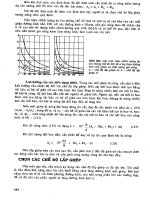
FIGURE 7.23
Average position
and extent of the
major surface ocean
currents. Cold cur-
rents are shown in
blue; warm currents
are shown in red.
Names of the ocean
currents are given in
Table 7.2.
1. Gulf Stream 9. South Equatorial Current 17. Peru or Humbolt Current
2. North Atlantic Drift 10. South Equatorial Countercurrent 18. Brazil Current
3. Labrador Current 11. Equatorial Countercurrent 19. Falkland Current
4. West Greenland Drift 12. Kuroshio Current 20. Benguela Current
5. East Greenland Drift 13. North Pacific Drift 21. Agulhas Current
6. Canary Current 14. Alaska Current 22. West Wind Drift

7. North Equatorial Current 15. Oyashio Current
8. North Equatorial Countercurrent 16. California Current
TABLE 7.2 Major Ocean Currents
WINDS AND UPWELLING Earlier, we saw that the cool
California Current flows roughly parallel to the west
coast of North America. From this, we might conclude
that summer surface water temperatures would be cool
along the coast of Washington and gradually warm as we
move south. A quick glance at the water temperatures
along the west coast of the United States during August
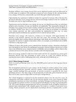
(Fig. 7.24) quickly alters that notion. The coldest water is
observed along the northern California coast near Cape
Mendocino. The reason for the cold, coastal water is
upwelling—the rising of cold water from below.
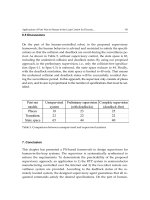
For upwelling to occur, the wind must flow more or
less parallel to the coastline. Notice in Fig. 7.25 that
summer winds tend to parallel the coastline of Califor-
nia. As the wind blows over the ocean, the surface water
beneath it is set in motion. As the surface water moves, it
bends slightly to its right due to the Coriolis effect.
(Remember, it would bend to the left in the Southern
Hemisphere.) The water beneath the surface also moves,
and it too bends slightly to its right. The net effect of this
phenomenon is that a rather shallow layer of surface
water moves at right angles to the wind and heads sea-
ward. As the surface water drifts away from the coast,
cold, nutrient-rich water from below rises (upwells) to
replace it. Upwelling is strongest and surface water is
coolest where the wind parallels the coast, such as it does
in summer along the coast of northern California.

Because of the cold coastal water, summertime
weather along the West Coast often consists of low
clouds and fog, as the air over the water is chilled to its
saturation point. On the brighter side, upwelling pro-
duces good fishing, as higher concentrations of nutri-
ents are brought to the surface. But swimming is only
for the hardiest of souls, since the average surface water
temperature in summer is nearly 10°C (18°F) colder
Global Wind Patterns and the Oceans 189
We have upwelling to thank for the famous quote of
Mark Twain: “The coldest winter I ever experienced was
a summer in San Francisco.”
6
Seattle
Portland
Cape Mendocino
San Francisco
Los Angeles
•
•
•
•
•
5
8
60
6
4
6
6

6
8
7
0
6
2
6
0
5
8
5
6
5
4
5
2
6
2
FIGURE 7.24
Average sea surface temperatures (°F) along the west coast of
the United States during August.
B
A
H
B
Coast range
58°
56°
54°
52°

Prevailing
summer
wind
A
W
i
n
d
FIGURE 7.25
As winds blow parallel to the west coast of North America, surface water is transported to the
right (out to sea). Cold water moves up from below (upwells) to replace the surface water.
than the average coastal water temperature found at the
same latitude along the Atlantic coast.
Between the ocean surface and the atmosphere, there
is an exchange of heat and moisture that depends, in part,
on temperature differences between water and air. In win-
ter, when air-water temperature contrasts are greatest,
there is a substantial transfer of sensible and latent heat
from the ocean surface into the atmosphere. This energy
helps to maintain the global airflow. Consequently, even
a relatively small change in surface ocean temperatures
could modify atmospheric circulations and have far-
reaching effects on global weather patterns. The next sec-
tion describes how weather events can be linked to surface
ocean temperature changes in the tropical Pacific.
EL NIÑO AND THE SOUTHERN OSCILLATION Along
the west coast of South America, where the cool Peru
Current sweeps northward, southerly winds promote up-
welling of cold, nutrient-rich water that gives rise to large
fish populations, especially anchovies. The abundance of

fish supports a large population of sea birds whose drop-
pings (called guano) produce huge phosphate-rich
deposits, which support the fertilizer industry. Near the
end of the calendar year, a warm current of nutrient-poor
tropical water often moves southward, replacing the cold,
nutrient-rich surface water. Because this condition fre-
quently occurs around Christmas, local residents call it El
Niño (Spanish for boy child), referring to the Christ child.
In most years, the warming lasts for only a few weeks
to a month or more, after which weather patterns usually
return to normal and fishing improves. However, when
El Niño conditions last for many months, and a more
extensive ocean warming occurs, the economic results can
be catastrophic. This extremely warm episode, which
occurs at irregular intervals of two to seven years and cov-
ers a large area of the tropical Pacific Ocean, is now
referred to as a major El Niño event, or simply El Niño.*
During a major El Niño event, large numbers of
fish and marine plants may die. Dead fish and birds may
litter the water and beaches of Peru; their decomposing
carcasses deplete the water’s oxygen supply, which leads
to the bacterial production of huge amounts of smelly
hydrogen sulfide. The El Niño of 1972–1973 reduced
the annual Peruvian anchovy catch from 10.3 million
metric tons in 1971 to 4.6 million metric tons in 1972.
Since much of the harvest of this fish is converted into
fishmeal and exported for use in feeding livestock and
poultry, the world’s fishmeal production in 1972 was
greatly reduced. Countries such as the United States
that rely on fishmeal for animal feed had to use soy-

beans as an alternative. This raised poultry prices in the
United States by more than 40 percent.
Why does the ocean become so warm over the east-
ern tropical Pacific? Normally, in the tropical Pacific
Ocean, the trades are persistent winds that blow west-
ward from a region of higher pressure over the eastern
Pacific toward a region of lower pressure centered near
Indonesia (see Fig. 7.26a). The trades create upwelling
that brings cold water to the surface. As this water moves
westward, it is heated by sunlight and the atmosphere.
Consequently, in the Pacific Ocean, surface water along
the equator usually is cool in the east and warm in the
west. In addition, the dragging of surface water by the
trades raises sea level in the western Pacific and lowers it
in the eastern Pacific, which produces a thick layer of
warm water over the tropical western Pacific Ocean and
a weak ocean current (called the countercurrent) that
flows slowly eastward toward South America.
Every few years, the surface atmospheric pressure
patterns break down, as air pressure rises over the region
of the western Pacific and falls over the eastern Pacific
(see Fig. 7.26b). This change in pressure weakens the
trades, and, during strong pressure reversals, east winds
are replaced by west winds. The west winds strengthen
the countercurrent, causing warm water to head east-
ward toward South America over broad areas of the
tropical Pacific. Toward the end of the warming period,
which may last between one and two years, atmospheric
pressure over the eastern Pacific reverses and begins to
rise, whereas, over the western Pacific, it falls. This see-

saw pattern of reversing surface air pressure at opposite
ends of the Pacific Ocean is called the Southern Oscilla-
tion. Because the pressure reversals and ocean warming
are more or less simultaneous, scientists call this phe-
nomenon the El Niño/Southern Oscillation or ENSO for
short. Although most ENSO episodes follow a similar
evolution, each event has its own personality, differing in
both strength and behavior.
During especially strong ENSO events (such as in
1982–83 and 1997–98) the easterly trades may actually
become westerly winds. As these winds push eastward,
they drag surface water with them. This dragging raises
sea level in the eastern Pacific and lowers sea level in the
western Pacific (see Fig. 7.26b). The eastward-moving
water gradually warms under the tropical sun, becom-
ing as much as 6°C (11°F) warmer than normal in the
eastern equatorial Pacific. Gradually, a thick layer of
warm water pushes into coastal areas of Ecuador and
190 Chapter 7 Atmospheric Circulations
*It was thought that El Niño was a local event that occurs along the west coast
of Peru and Ecuador. It is now known that the ocean-warming associated
with a major El Niño can cover an area of the tropical Pacific much larger
than the continental United States.
Peru, choking off the upwelling that supplies cold,
nutrient-rich water to South America’s coastal region.
The unusually warm water may extend from South
America’s coastal region for many thousands of kilome-
ters westward along the equator (see Fig. 7.27). The
warm tropical water may even spread northward along
the west coast of North America.

Such a large area of abnormally warm water can
have an effect on global wind patterns. The warm tropi-
cal water fuels the atmosphere with additional warmth
and moisture, which the atmosphere turns into addi-
tional storminess and rainfall. The added warmth from
the oceans and the release of latent heat during conden-
sation apparently influence the westerly winds aloft in
such a way that certain regions of the world experience
too much rainfall, whereas others have too little. Mean-
while, over the warm tropical central Pacific, the fre-
quency of typhoons usually increases. However, over the
tropical Atlantic, between Africa and Central America,
the winds aloft tend to disrupt the organization of thun-
derstorms that is necessary for hurricane development;
hence, there are fewer hurricanes in this region during
strong El Niño events. And, as we saw earlier in this chap-
ter, during a strong El Niño, summer monsoon condi-
tions tend to weaken over India, although this weakening
did not happen during the strong El Niño of 1997.
Although the actual mechanism by which changes
in surface ocean temperatures influence global wind
patterns is not fully understood, the by-products are
plain to see. For example, during exceptionally warm
El Niños, drought is normally felt in Indonesia, southern
Africa, and Australia, while heavy rains and flooding
often occur in Ecuador and Peru. In the Northern Hemi-
sphere, a strong subtropical westerly jet stream normally
directs storms into California and heavy rain into the
Gulf Coast states. The total damage worldwide due to
flooding, winds, and drought may exceed $8 billion.

Following an ENSO event, the trade winds usually
return to normal. However, if the trades are exceptionally
strong, unusually cold surface water moves over the
Global Wind Patterns and the Oceans 191
Equator
Indonesia
Warm water
L
WET
Strong trade winds
Cool water
Upwelling
EASTWEST
Warm water
Thermocline
50 m
200 m
Cold water
Sinking air
0
DRY
H
(a) Non-El Niño Conditions
Sinking air
DRY
Atmospheric
pressure rises
Strong counter current
Atmospheric
pressure falls

Thermocline
Warm water
EASTWEST
Peru
Ocean level
rises
Equator
WET
(b) El Niño Conditions
Ecuador
Peru
Ocean
water
level
higher
FIGURE 7.26
In diagram (a), under ordinary con-
ditions higher pressure over the
southeastern Pacific and lower pres-
sure near Indonesia produce easterly
trade winds along the equator.
These winds promote upwelling and
cooler ocean water in the eastern
Pacific, while warmer water prevails
in the western Pacific. The trades are
part of a circulation that typically
finds rising air and heavy rain over
the western Pacific and sinking air
and generally dry weather over the
eastern Pacific. When the trades are

exceptionally strong, water along
the equator in the eastern Pacific
becomes quite cool. This cool event
is called La Niña. During El Niño
conditions—diagram (b)—atmo-
spheric pressure decreases over the
eastern Pacific and rises over the
western Pacific. This change in pres-
sure causes the trades to weaken or
reverse direction. This situation
enhances the countercurrent that
carries warm water from the west
over a vast region of the eastern
tropical Pacific. The thermocline,
which separates the warm water of
the upper ocean from the cold water
below, changes as the ocean con-
ditions change from non-El Niño
to El Niño.
central and eastern Pacific, and the warm water and rainy
weather is confined mainly to the western tropical Pacific.
This cold-water episode, which is the opposite of El Niño
conditions, has been termed La Niña (the girl child).
As we have seen, El Niño and the Southern Oscilla-
tion are part of a large-scale ocean-atmosphere interac-
tion that can take several years to run its course. During
this time, there are certain regions in the world where
significant climatic responses to an ENSO event are
likely. Using data from previous ENSO episodes, scien-
tists at the National Oceanic and Atmospheric Admin-

istration’s Climatic Prediction Center have obtained a
global picture of where climatic abnormalities are most
likely (see Fig. 7.28).
Some scientists feel that the trigger necessary to
start an ENSO event lies within the changing of the sea-
sons, especially the transition periods of spring and fall.
Others feel that the winter monsoon plays a major role
in triggering a major El Niño event. As noted earlier, it
appears that an ENSO episode and the monsoon system
are intricately linked, so that a change in one brings
about a change in the other.
Presently, scientists (with the aid of coupled general
circulation models) are trying to simulate atmospheric
and oceanic conditions, so that El Niño and the Southern
Oscillation can be anticipated. At this point, several mod-
els have been formulated that show promise in predicting
the onset and life history of an ENSO event. In addition,
an in-depth study known as TOGA (Tropical Ocean and
Global Atmosphere), which began in 1985 and ended in
1994, is providing scientists with valuable information
about the interactions that occur between the ocean and
the atmosphere. The primary aim of TOGA, a major
component of the World Climate Research Program
(WCRP), is to provide enough scientific information so
that researchers can better predict climatic fluctuations
(such as ENSO) that occur over periods of months and
years. The hope is that a better understanding of El Niño
and the Southern Oscillation will provide improved
long-range forecasts of weather and climate.
192 Chapter 7 Atmospheric Circulations

FIGURE 7.27
Sea surface temperature (SSTs) as
measured by satellites. During non-
El Niño conditions—diagram (a)—
upwelling along the equator and coast
of Peru keeps the water cool (blue
colors) in the tropical eastern Pacific.
During El Niño conditions—diagram
(b)—upwelling is greatly diminished,
and warm water (deep red color) from
the western Pacific has replaced the
cool water.
(a)
(b)
Summary
In this chapter, we examined a variety of atmospheric
circulations. We looked at small-scale winds and found
that eddies can form in a region of strong wind shear,
especially in the vicinity of a jet stream. On a slightly
larger scale, land and sea breezes blow in response to
local pressure differences created by the uneven heating
and cooling rates of land and water. Monsoon winds
change direction seasonally, while mountain and valley
winds change direction daily.
A warm, dry wind that descends the eastern side of
the Rocky Mountains is the chinook. The same type of
wind in the Alps is the foehn. A warm, dry downslope
wind that blows into southern California is the Santa
Ana wind. Local intense heating of the surface can pro-
duce small rotating winds, such as the dust devil, while

downdrafts in a thunderstorm are responsible for the
desert haboob.
The largest pattern of winds that persists around the
globe is called the general circulation. At the surface in
both hemispheres, winds tend to blow from the east in the
tropics, from the west in the middle latitudes, and from
the east in polar regions. Where upper-level westerly
Summary 193
90 180 90 0
Longitude
60
30
0
30
60
Latitude
60
30
0
30
90
180 90 0
90
90
60
Nov. – Mar.
Jun. – Nov.
Sep. – Mar.
Mar. – Feb.
May – Oct.

Nov. – May
May – Apr.
Jul. – Jun.
Dec. – Mar.
Apr. – Oct.
Oct. – Mar.
Nov. – Mar.
Jul. – Oct.
Jul. – Mar.
Nov. – Feb.
Nov. – Mar.
Nov. – May
Sep. – May
Jun. – Sep.
Oct. – Dec.
LEGEND
Dry
Wet
Warm
FIGURE 7.28
Regions of climatic abnormalities associated with El Niño–Southern Oscillation conditions. A strong ENSO
event may trigger a response in nearly all indicated areas, whereas a weak event will likely play a role in only
some areas. Note that the months in black type indicate months during the same years the major warming
began; months in red type indicate the following year. (After NOAA Climatic Prediction Center.)
winds tend to concentrate into narrow bands, we find jet
streams. The annual shifting of the major pressure sys-
tems and wind belts—northward in July and southward
in January—strongly influences the annual precipitation
of many regions.
Toward the end of the chapter we examined the

interaction between the atmosphere and oceans. Here we
found the interaction to be an ongoing process where
everything, in one way or another, seems to influence
everything else. On a large scale, winds blowing over the
surface of the water drive the major ocean currents;
the oceans, in turn, release energy to the atmosphere,
which helps to maintain the general circulation. When
atmospheric circulation patterns change, and the trade
winds weaken or reverse direction, warm tropical water is
able to flow eastward toward South America where it
chokes off upwelling and produces disasterous economic
conditions. When the warm water extends over a vast
area of the Tropical Pacific, the warming is called a major
El Niño event, and the associated reversal of pressure over
the Pacific Ocean is called the Southern Oscillation. The
large-scale interaction between the atmosphere and the
ocean during El Niño and the Southern Oscillation
(ENSO) affects global atmospheric circulation patterns.
The sweeping winds aloft provide too much rain in some
areas and not enough in others. Studies now in progress
are designed to determine how the interchange between
atmosphere and ocean can produce such events.
Key Terms
The following terms are listed in the order they appear in
the text. Define each. Doing so will aid you in reviewing
the material covered in this chapter.
Questions for Review
1. Describe the various scales of motion and give an
example of each.
2. What is wind shear and how does it relate to clear air

turbulance?
3. Using a diagram, explain how a thermal circulation
develops.
4. Why does a sea breeze blow from sea to land and a
land breeze from land to sea?
5. (a) Briefly explain how the monsoon wind system
develops over eastern and southern Asia.
(b) Why in India is the summer monsoon wet and
the winter monsoon dry?
6. Which wind will produce clouds: a valley breeze or a
mountain breeze? Why?
7. What are katabatic winds? How do they form?
8. Explain why chinook winds are warm and dry.
9. (a) What is the primary source of warmth for a
Santa Ana wind?
(b) What atmospheric conditions contribute to the
development of a strong Santa Ana?
10. What weather conditions are conducive to the forma-
tion of dust devils?
11. Draw a large circle. Now, place the major surface
semipermanent pressure systems and the wind belts of
the world at their appropriate latitudes.
12. According to Fig. 7.15 (p.
180), most of the United
States is located in what wind belt?
13. Explain how and why the average surface pressure fea-
tures shift from summer to winter.
14. Explain the relationship between the general circula-
tion of air and the circulation of ocean currents.
15. (a) Is the polar jet stream or the subtropical jet

stream normally observed at a lower elevation?
(b) In the Northern Hemisphere, which of the two jet
streams is typically observed at lower latitudes?
16. Why is the polar jet stream more strongly developed
in winter?
17. Describe how the winds along the west coast of North
America produce upwelling.
194 Chapter 7 Atmospheric Circulations
scales of motion
microscale
mesoscale
synoptic scale
planetary scale
rotor
wind shear
clear air turbulence (CAT)
thermal circulation
sea breeze
land breeze
monsoon wind system
valley breeze
mountain breeze
katabatic wind
chinook wind
Santa Ana wind
haboob
dust devils (whirlwinds)
general circulation of the
atmosphere
Hadley cell

doldrums
subtropical highs
trade winds
intertropical convergence
zone (ITCZ)
westerlies
polar front
subpolar low
polar easterlies
Bermuda high
Pacific high
Icelandic low
Aleutian low
Siberian high
jet stream
subtropical jet stream
polar front jet stream
upwelling
El Niño
Southern Oscillation
ENSO
La Niña
18. (a) What is a major El Niño event?
(b) What happens to the surface pressure at opposite
ends of the Pacific Ocean during the Southern
Oscillation?
(c) Describe how an ENSO event may influence the
weather in different parts of the world.
19.
What are the conditions over the tropical eastern

and central Pacific Ocean during the phenomenon
known as La Niña?
Questions for Thought
and Exploration
1. Suppose you are fishing in a mountain stream during
the early morning. Is the wind more likely to be blow-
ing upstream or downstream? Explain why.
2. Why, in Antarctica, are winds on the high plateaus usu-
ally lighter than winds in steep, coastal valleys?
3. What atmospheric conditions must change so that the
westerly flowing polar-front jet stream reverses direc-
tion and becomes an easterly flowing jet stream?
4. Swimmers will tell you that surface water temperatures
along the eastern shore of Lake Michigan are usually
much cooler than surface water temperatures along the
western shore. Give the swimmers a good (logical)
explanation for this temperature variation.
5. Use the Atmospheric Circulation/Global Atmosphere
section of the Blue Skies CD-ROM to observe a one-
week animation of global winds and cloud cover. Iden-
tify the location of the intertropical convergence zone,
the trade winds, and the prevailing westerlies.
6. Use the Atmospheric Circulation/Global Ocean section
of the Blue Skies CD-ROM to observe ocean currents
throughout the year. Is the mixing of warm water with
cold water evenly distributed around the ocean or
focused on certain regions? What features can you
observe that may be important to the exchange of heat
from the tropics to the polar regions?
7. Use the Atmospheric Circulation/Southern Oscillation

section of the Blue Skies CD-ROM to examine the rela-
tionship between ocean temperature and precipitation
over land. What relationships can you see between the
movement of warm water in the Pacific Ocean and wet
and dry patterns on the continents?
8. Pacific and Atlantic satellite images (http://www.
earthwatch.com/WX_HDLINES/tropical.html): Exam-
ine current infrared satellite images of the Pacific and
Atlantic Ocean regions. Describe the types and sizes of
the eddies that appear in the images.
9. Local Winds ( />local.htm): Look up several local wind circulations that
affect specific localized areas around the globe.
For additional readings, go to InfoTrac College
Edition, your online library, at:

Questions for Thought and Exploration 195

Air Masses
Source Regions
Classification
Air Masses of North America
cP (Continental Polar) and cA
(Continental Arctic) Air Masses
Focus on a Special Topic:
Lake-Effect (Enhanced) Snows
mP (Maritime Polar) Air Masses
Focus on a Special Topic:
The Return of the Siberian Express
mT (Maritime Tropical) Air Masses
cT (Continental Tropical) Air Masses

Fronts
Stationary Fronts
Cold Fronts
Warm Fronts
Occluded Fronts
Middle-Latitude Cyclones
Polar Front Theory
Where Do Mid-Latitude Cyclones
Tend to Form?
Developing Mid-Latitude Cyclones
and Anticyclones
Focus on a Special Topic:
Northeasters
Focus on a Special Topic:
A Closer Look at Convergence
and Divergence
Jet Streams and Developing
Mid-Latitude Cyclones
Focus on a Special Topic:
Waves in the Westerlies
Summary
Key Terms
Questions for Review
Questions for Thought and Exploration
Contents
A
bout two o’clock in the afternoon it began to grow
dark from a heavy, black cloud which was seen in
the northwest. Almost instantly the strong wind, traveling at the
rate of 70 miles an hour, accompanied by a deep bellowing

sound, with its icy blast, swept over the land, and everything
was frozen hard. The water in the little ponds in the roads
froze in waves, sharp edged and pointed, as the gale had
blown it. The chickens, pigs and other small animals were
frozen in their tracks. Wagon wheels ceased to roll, froze to
the ground. Men, going from their barns or fields a short
distance from their homes, in slush and water, returned a few
minutes later walking on the ice. Those caught out on
horseback were frozen to their saddles, and had to be lifted off
and carried to the fire to be thawed apart. Two young men
were frozen to death near Rushville. One of them was found
with his back against a tree, with his horse’s bridle over his
arm and his horse frozen in front of him. The other was partly
in a kneeling position, with a tinder box in one hand and a flint
in the other, with both eyes wide open as if intent on trying to
strike a light. Many other casualties were reported. As to the
exact temperature, however, no instrument has left any record;
but the ice was frozen in the stream, as variously reported,
from six inches to a foot in thickness in a few hours.
John Moses, Illinois: Historical and Statistical
Air Masses, Fronts, and Middle-Latitude Cyclones
197
T
he opening details the passage of a spectacular
cold front as it moved through Illinois on Decem-
ber 21, 1836. Although no reliable temperature records
are available, estimates are that, as the front swept
through, air temperatures dropped almost instantly from
the balmy 40s (°F) to 0 degrees. Fortunately, temperature
changes of this magnitude are quite rare with cold fronts.

In this chapter, we will examine the more typical
weather associated with cold fronts and warm fronts. We
will address questions such as: Why are cold fronts usu-
ally associated with showery weather? How can warm
fronts cause freezing rain and sleet to form over a vast
area during the winter? And how can one read the story
of an approaching warm front by observing its clouds?
We will also see how weather fronts are an integral part
of a mid-latitude cyclonic storm. But, first, so that we
may better understand fronts and storms, we will exam-
ine air masses. We will look at where and how they form
and the type of weather usually associated with them.
Air Masses
An air mass is an extremely large body of air whose
properties of temperature and humidity are fairly simi-
lar in any horizontal direction at any given altitude. Air
masses may cover many thousands of square kilometers.
In Fig. 8.1, a large winter air mass, associated with a
high pressure area, covers over half of the United States.
Note that, although the surface air temperature and dew
point vary somewhat, everywhere the air is cold and
dry, with the exception of the zone of snow showers on
the eastern shores of the Great Lakes. This cold, shallow
anticyclone will drift eastward, carrying with it the tem-
perature and moisture characteristic of the region
where the air mass formed; hence, in a day or two, cold
air will be located over the central Atlantic Ocean. Part
of weather forecasting is, then, a matter of determining
air mass characteristics, predicting how and why they
change, and in what direction the systems will move.

SOURCE REGIONS Regions where air masses originate
are known as source regions. In order for a huge mass
of air to develop uniform characteristics, its source
region should be generally flat and of uniform compo-
sition, with light surface winds. The longer the air
remains stagnant over its source region, the more likely
it will acquire properties of the surface below. Conse-
quently, ideal source regions are usually those areas
dominated by high pressure. They include the ice- and
snow-covered arctic plains in winter and subtropical
oceans and desert regions in summer. The middle lati-
tudes, where surface temperatures and moisture charac-
teristics vary considerably, are not good source regions.
Instead, this region is a transition zone where air masses
198 Chapter 8 Air Masses, Fronts, and Middle-Latitude Cyclones
12
7
1020
1024
–5
–10
14
1
18
10
10
0
–15
–18
–15

–32
–5
–16
1016
7
–6
–9
–11
10
7
1032
16
12
43
39
27
18
9
–2
25
14
–18
–20
–13
–18
–15
–24
1
–9
–8

–15
–17
–20
14
5
Philadelphia
1024
3
–2
28
18
Pittsburgh
–2
–9
1028
H
1016
1020
FIGURE 8.1
Here, a large, extremely cold
winter air mass is dominating the
weather over much of the United
States. At almost all cities, the air is
cold and dry. Upper number is air
temperature (°F); bottom number
is dew point (°F).
with different physical properties move in, clash, and
produce an exciting array of weather activity.
CLASSIFICATION Air masses are grouped into four
general categories according to their source region. Air

masses that originate in polar latitudes are designated
by the capital letter P (for Polar); those that form in
warm tropical regions are designated by the capital let-
ter T (for Tropical). If the source region is land, the air
mass will be dry and the lowercase letter c (for continen-
tal) precedes the P or T. If the air mass originates over
water, it will be moist—at least in the lower layers—and
the lowercase letter m (for maritime) precedes the P or
T. We can now see that polar air originating over land
will be classified cP on a surface weather chart, while
tropical air originating over water will be marked as mT.
In winter, an extremely cold cP air mass is designated as
cA, continental arctic. Often, however, it is difficult to
distinguish between arctic and polar air masses, espe-
cially when the arctic air mass has traveled over warmer
terrain. By the same token, an extremely hot, humid air
mass originating over equatorial waters is sometimes
designated as mE, for maritime equatorial. Distinguish-
ing between equatorial and tropical air masses is usually
difficult. Table 8.1 lists the four basic air masses.
When the air mass is colder than the underlying
surface, it is warmed from below, which makes the
air unstable at low levels. In this case, increased convec-
tion and turbulent mixing near the surface usually pro-
duce good visibility, cumuliform clouds, and showers of
rain or snow. On the other hand, when the air mass is
warmer than the surface below, the lower layers are
chilled by contact with the cold earth. Warm air above
cooler air produces stable air with little vertical mixing.
This situation causes the accumulation of dust, smoke,

and pollutants, which restricts surface visibilities. In
moist air, stratiform clouds accompanied by drizzle or
fog may form.
AIR MASSES OF NORTH AMERICA The principal air
masses (with their source regions) that invade the United
States are shown in Fig. 8.2. We are now in a position to
study the formation and modification of each of these air
masses and the variety of weather that accompanies them.
cP (Continental Polar) and cA (Continental Arctic) Air
Masses The bitterly cold weather that enters the
United States in winter is associated with continental
polar and continental arctic air masses. These originate
over the ice- and snow-covered regions of northern
Canada and Alaska where long, clear nights allow for
strong radiational cooling of the surface. Air in contact
with the surface becomes quite cold and stable. Since
little moisture is added to the air, it is also quite dry.
Eventually a portion of this cold air breaks away and,
under the influence of the airflow aloft, moves south-
ward as an enormous shallow high pressure area.
As the cold air moves into the interior plains, there
are no topographic barriers to restrain it, so it continues
southward, bringing with it cold wave warnings and
frigid temperatures. As the air mass moves over warmer
land to the south, the air temperature moderates slightly.
However, even during the afternoon, when the surface
air is most unstable, cumulus clouds are rare because of
the extreme dryness of the air mass. At night, when the
winds die down, rapid surface cooling and clear skies
Air Masses 199

Land cP cT
continental Cold, dry, stable Hot, dry, stable
(c) air aloft;
unstable
surface air
Water mP mT
maritime Cool, moist, Warm, moist;
(m) unstable usually unstable
TABLE 8.1
Air Mass Classification and Characteristics
Source Region Polar (P) Tropical (T)
cT
Summer only
mT
mP
mT
mP
cA
mT
cP
FIGURE 8.2
Air mass source regions and their paths.
combine to produce low minimum temperatures. If the
cold air moves as far south as central or southern
Florida, the winter vegetable crop may be severely dam-
aged. When the cold, dry air mass moves over a relatively
warm body of water, such as the Great Lakes, heavy snow
showers—called lake-effect snows—often form on the
eastern shores. (More information on lake-effect snows
is provided in the Focus section above.)

In winter, the generally fair weather accompanying
cP air is due to the stable nature of the atmosphere aloft.
200 Chapter 8 Air Masses, Fronts, and Middle-Latitude Cyclones
During the winter, when the weather
in the Midwest is dominated by
clear, brisk cP (or cA) air, people liv-
ing on the eastern shores of the
Great Lakes brace themselves for
heavy snow showers. Snowstorms
that form on the downwind side of
one of these lakes are known as
lake-effect snows. (Since the lakes
are responsible for enhancing the
amount of snow that falls, these
snowstorms are also called lake-
enhanced snows.) Such storms are
highly localized, extending from just
a few kilometers to more than 50 km
inland. The snow usually falls as a
heavy shower or squall in a concen-
trated zone. So centralized is the
region of snowfall, that one part of a
city may accumulate many centi-
meters of snow, while, in another
part, the ground is bare.
Lake-effect snows are most
numerous from November to January.
During these months, cP air moves
over the lakes when they are relatively
warm and not quite frozen. The

contrast in temperature between water
and air can be as much as 25°C
(45°F). Studies show that the greater
the contrast in temperature, the greater
the potential for snow showers. In Fig.
1, we can see that, as the cold air
moves over the warmer water, the air
mass is quickly warmed from below,
making it more buoyant and less
stable. Rapidly, the air sweeps up
moisture, soon becoming saturated.
Out over the water, the vapor
condenses into steam fog. As the air
continues to warm, it rises and forms
billowing cumuliform clouds, which
continue to grow as the air becomes
more unstable. Eventually, these clouds
produce heavy showers of snow,
which make the lake seem like a snow
factory. Once the air and clouds reach
the downwind side of the lake, addi-
tional lifting is provided by low hills
and the convergence of air as it slows
down over the rougher terrain. In late
winter, the frequency and intensity of
lake-effect snows taper off as the
temperature contrast between water
and air diminishes and larger portions
of the lakes freeze.
Generally, the longer the stretch of

water over which the air mass travels
(the longer the fetch), the greater the
amount of warmth and moisture
derived from the lake, and the greater
the potential for heavy snow showers.
Consequently, forecasting lake-effect
snowfalls depends to a large degree
on determining the trajectory of the
air as it flows over the lake. Regions
that experience heavy lake-effect
snowfalls are shown in Fig. 2.
As the cP air moves farther east, the
heavy snow showers usually taper off;
however, the western slope of the
Appalachian Mountains produces
further lifting, enhancing the possibility
of more and heavier showers. The
heat given off during condensation
warms the air and, as the air descends
the eastern slope, compressional heat-
ing warms it even more. Snowfall
ceases, and by the time the air arrives
at Philadelphia, New York, or Boston,
the only remaining trace of the snow
showers occurring on the other side of
the mountains are the puffy cumulus
clouds drifting overhead.
Lake-effect (or enhanced) snows are
not confined to the Great Lakes. In
fact, any large unfrozen lake (such as

the Great Salt Lake) can enhance
snowfall when cold, relatively dry air
sweeps over it.
LAKE-EFFECT (ENHANCED) SNOWS
Focus on a Special Topic
Evaporation and warmth
Warm water
cP
Air mass
Leeward
Windward
Fog
FIGURE 1
The formation of lake-effect snows. Cold, dry air crossing the lake gains moisture
and warmth from the water. The more buoyant air now rises, forming clouds that
deposit large quantities of snow on the lake’s leeward shores.
WI
IL
IN
OH
MI
NY
PA
FIGURE 2
Areas shaded purple show regions that
experience heavy lake-effect snows.
Sinking air develops above the large dome of high pres-
sure. The subsiding air warms by compression and cre-
ates warmer air, which lies above colder surface air.
Therefore, a strong upper-level temperature inversion

often forms. Should the anticyclone stagnate over a
region for several days, the visibility gradually drops as
pollutants become trapped in the cold air near the
ground. Usually, however, winds aloft move the cold air
mass either eastward or southeastward.
The Rockies, Sierra Nevada, and Cascades nor-
mally protect the Pacific Northwest from the onslaught
of cP air, but, occasionally, cP air masses do invade these
regions. When the upper-level winds over Washington
and Oregon blow from the north or northeast on a tra-
jectory beginning over northern Canada or Alaska, cold
cP (and cA) air can slip over the mountains and extend
its icy fingers all the way to the Pacific Ocean. As the air
moves off the high plateau, over the mountains, and on
into the lower valleys, compressional heating of the
sinking air causes its temperature to rise, so that by the
time it reaches the lowlands, it is considerably warmer
than it was originally. However, in no way would this air
be considered warm. In some cases, the subfreezing
temperatures slip over the Cascades and extend south-
ward into the coastal areas of southern California.
A similar but less dramatic warming of cP and cA
air occurs along the east coast of the United States. Air
rides up and over the lower Appalachian Mountains.
Turbulent mixing and compressional heating increase
the air temperatures on the downwind side. Conse-
quently, cities located to the east of the Appalachian
Mountains usually do not experience temperatures as
low as those on the west side. In Fig. 8.1, notice that for
the same time of day—in this case 7

A.M. EST—
Philadelphia, with an air temperature of 14°F, is 16°F
warmer than Pittsburgh, at –2°F.
Figure 8.3 shows two upper-air patterns that led to
extremely cold outbreaks of arctic air during December
1989 and 1990. Upper-level winds typically blow from
west to east, but, in both of these cases, the flow, as given
by the heavy, dark arrows, had a strong north-south
(meridional) trajectory. The H represents the positions of
the cold surface anticyclones. Numbers on the map rep-
resent minimum temperatures (°F) recorded during the
cold spells. East of the Rocky Mountains, over 350 record
low temperatures were set between December 21 and 24,
Air Masses 201
–38
–23
13
1
23
13
20
21
–21
–28
–29
–34
–40
–30
–29
–23

–20
–5
8
14
–13
–12
–15
–15
12/23/89
5
11
9
–12
–11
15
16
22
31
13
–6
H
H
H
H
H
–14
2
14
–28
–47

12/20/90
12/21/89
–28
12/22/89
–25
12/22/90
38
18
8
9
FIGURE 8.3
Average upper-level wind flow
(heavy arrows) and surface
position of anticyclones (H)
associated with two extremely
cold outbreaks of arctic air during
December. Numbers on the map
represent minimum temperatures
(°F) measured during each cold
snap.
Montague, New York, which lies on the eastern side of
Lake Ontario, became buried under lake-effect snow
when, during January, 1997, it received 218 cm
(86 in.) of snow in less than 48 hours. An astounding
195 cm (77 in.) fell during the first 24 hours. But, appar-
ently, this is not a national record as there seems to be
some concern about the frequency of snow measurement
during the storm.
1989, with the arctic outbreak causing an estimated $480
million in damage to the fruit and vegetable crops in

Texas and Florida. Along the West Coast, the frigid air
during December, 1990, caused over $300 million in
damage to the vegetable and citrus crops, as temperatures
over parts of California plummeted to their lowest read-
ings in more than fifty years. Notice in both cases how the
upper-level wind directs the paths of the air masses.
The cP air that moves into the United States in
summer has properties much different from its winter
counterpart. The source region remains the same but is
now characterized by long summer days that melt snow
and warm the land. The air is only moderately cool, and
surface evaporation adds water vapor to the air. A sum-
mertime cP air mass usually brings relief from the
oppressive heat in the central and eastern states, as
cooler air lowers the air temperature to more comfort-
able levels. Daytime heating warms the lower layers,
producing surface instability. With its added moisture,
the rising air may condense and create a sky dotted with
fair weather cumulus clouds.
When an air mass moves over a large body of
water, its original properties may change considerably.
For instance, cold, dry cP air moving over the Gulf of
Mexico warms rapidly and gains moisture. The air
quickly assumes the qualities of a maritime air mass.
Notice in Fig. 8.4 that rows of cumulus clouds are form-
ing over the Gulf of Mexico parallel to northerly surface
winds as cP air is being warmed by the water beneath it.
As the air continues its journey southward into Mexico
and Central America, strong, moist northerly winds
build into heavy clouds (bright area) and showers along

the northern coast. Hence, a once cold, dry, and stable
air mass can be modified to such an extent that its orig-
inal characteristics are no longer discernible. When this
happens, the air mass is given a new designation.
In summary, polar and arctic air masses are respon-
sible for the bitter cold winter weather that can cover
wide sections of North America. When the air mass orig-
inates over the Canadian Northwest Territories, frigid air
can bring record-breaking low temperatures. Such was
the case on Christmas Eve, 1983, when arctic air covered
most of North America. (A detailed look at this air mass
and its accompanying record-setting low temperatures is
given in the Focus section on p. 203.)
mP (Maritime Polar) Air Masses During the winter,
cP air originating over Asia and frozen polar regions is
carried eastward and southward over the Pacific Ocean
by the circulation around the Aleutian low. The ocean
water modifies the cP air by adding warmth and mois-
ture to it. Since this air has to travel over water many
202 Chapter 8 Air Masses, Fronts, and Middle-Latitude Cyclones
cP
cP
FIGURE 8.4
Visible satellite image showing the
modification of cP air as it moves
over the warmer Gulf of Mexico
and the Atlantic Ocean.
Air Masses 203
The winter of 1983–1984 was one of the
coldest on record across North America.

Unseasonably cold weather arrived in
December, which, for much of the country,
was one of the coldest Decembers since
records have been kept. During the first
part of the month, continental polar air
covered most of the northern and central
plains. As the cold air moderated slightly,
far to the north a huge mass of bitter cold
arctic air was forming over the frozen
reaches of the Canadian Northwest
Territories.
By mid-month, the frigid air, associated
with a massive high pressure area, cover-
ed all of northwest Canada. Meanwhile,
aloft, strong northerly winds directed the
leading edge of the frigid air southward
over the prairie provinces of Canada and
southward into the United States. Because
the extraordinarily cold air was accom-
panied in some regions by winds gusting
to 45 knots, at least one news reporter
dubbed the onslaught of this arctic blast,
“the Siberian Express.”
The Express dropped temperatures to
some of the lowest readings ever recorded
during the month of December. On Decem-
ber 22, Elk Park, Montana, recorded an
unofficial low of –53°C (–64°F), only 4°C
higher than the all-time low of –57°C
(–70°F) for the nation (excluding Alaska)

recorded at Rogers Pass, Montana, on Jan-
uary 20, 1954.
The center of the massive anticyclone
gradually pushed southward out of
Canada. By December 24, its center was
over eastern Montana (Fig. 3), where the
sea level pressure at Miles City reached
an incredible 1064 mb (31.42 in.)—a
new United States record that topped the
old mark of 1063 mb set in Helena, Mon-
tana, on January 10, 1962. An enormous
ridge of high pressure stretched from the
Canadian arctic coast to the Gulf of Mex-
ico. On the east side of the ridge, cold
westerly winds brought lake-effect snows
to the eastern shores of the Great Lakes.
To the south of the high pressure center,
cold easterly winds, rising along the
elevated plains, brought light amounts of
upslope snow* to sections of the Rocky
Mountain states. Notice in Fig. 3 that, on
Christmas Eve, arctic air covered almost
90 percent of the United States. As the
cold air swept eastward and southward, a
hard freeze caused hundreds of millions
of dollars in damage to the fruit and vege-
table crops in Texas, Louisiana, and
Florida. On Christmas Day, 125 record
low temperature readings were set in
twenty-four states. That afternoon, at

1:00
P.M., it was actually colder in
Atlanta, Georgia, than it was in Fair-
banks, Alaska. One of the worst cold
waves to occur in December during this
century continued through the week, as
many new record lows were established
in the Deep South from Texas to Louisiana.
By January 1, the extreme cold had
moderated, as the upper-level winds
became more westerly. These winds
brought milder mP Pacific air eastward
into the Great Plains. The warmer pattern
continued until about January 10, when
the Siberian Express decided to make a
return visit. Driven by strong upper-level
northerly winds, impulse after impulse of
arctic air from Canada swept across the
United States. On January 18, an all-time
record low of –54°C (–65°F) was
recorded for the state of Utah at Middle
Sinks. On January 19, temperatures plum-
THE RETURN OF THE SIBERIAN EXPRESS
Focus on a Special Topic
*Upslope snow forms as cold air moving from east
to west gradually rises (and cools even more) as it
approaches the Rocky Mountains.
FIGURE 3
Surface weather map for 7 A.M., EST, December 24, 1983. Solid lines are isobars. Areas
shaded green represent precipitation. An extremely cold arctic air mass covers nearly 90 per-

cent of the United States. (Weather symbols for the surface map are given in Appendix B.)
1000
–30
–39
–19
–29
1004
16
13
10
5
1008
20
5
–16
–29
1048
1064
–22
–27
–18
–33
–16
–26
1052
–15
–26
5
–5
12

5
10
–6
–14
–29
–37
17
–20
1056
1060
H
1012
1016
18
10
36
28
12
8
–23
33
1020
1044
1040
1036
16
3
1032
1016
53

43
49
44
1012
1008
1004
1020
1024
1028
1032
6
meted to a new low of –22°C (–7°F) for
the airports in Philadelphia and Baltimore.
Toward the end of the month, the upper-
level winds once again became more
westerly. Over much of the nation, the
cold air moderated. But the Express was
to return at least one more time.
The beginning of February saw rela-
tively warm air covering much of the
nation from California to the Atlantic coast.
On February 4, an arctic outbreak of cA
air spread southward and eastward across
the nation. Although freezing air extended
southward into central Florida, the Express
ran out of steam, and a February heat
wave soon engulfed most of the United
States east of the Rocky Mountains. Mari-
time tropical air from the Gulf of Mexico
brought record warmth to much of the east-

ern two-thirds of the nation. Near the mid-
dle of the month, Louisville, Kentucky,
reported 23°C (73°F) and Columbus,
Ohio, 21°C (69°F). Even though February
was one of the warmest months on record
over parts of the United States, the winter
of 1983–1984 (December, January, and
February) will go down in the record
books as one of the coldest winters for the
United States as a whole since reliable
record keeping began in 1931.
hundreds or even thousands of kilometers, it gradually
changes into a maritime polar air mass.
By the time this air mass reaches the Pacific coast it
is cool, moist, and conditionally unstable. The ocean’s
effect is to keep air near the surface warmer than the air
aloft. Temperature readings in the 40s and 50s (°F) are
common near the surface, while air at an altitude of
about a kilometer or so above the surface may be at the
freezing point. Within this colder air, characteristics of
the original cP air mass may still prevail. As the air moves
inland, coastal mountains force it to rise, and much of its
water vapor condenses into rain-producing clouds. In the
colder air aloft, the rain changes to snow, with heavy
amounts accumulating in mountain regions. A typical
upper-level wind flow pattern that brings mP air onto the
west coast of North America is shown in Fig. 8.5.
When the mP air moves inland, it loses much of its
moisture as it crosses a series of mountain ranges. Beyond
these mountains, it travels over a cold, elevated plateau

that chills the surface air and slowly transforms the lower
level into a drier, more stable air mass. East of the Rock-
ies this air mass is referred to as Pacific air (see Fig. 8.6).
Here, it often brings fair weather and temperatures that
are cool but not nearly as cold as the cP air that invades
this region from northern Canada. In fact, when mP air
from the west replaces retreating cP air from the north,
chinook winds often develop. Furthermore, when the
modified mP air replaces moist tropical air, storms can
form along the boundary separating the two air masses.
Along the East Coast, mP air originates in the
North Atlantic as cP air moves southward some distance
off the Atlantic coast. Steered by northeasterly winds,
mP air then swings southwestward toward the north-
eastern states. Because the water of the North Atlantic is
very cold and the air mass travels only a short distance
over water, wintertime Atlantic mP air masses are usu-
ally much colder than their Pacific counterparts.
Because the prevailing winds aloft are westerly, Atlantic
mP air masses are also much less common.
Figure 8.7 illustrates a typical late winter or early
spring surface weather pattern that carries mP air from
the Atlantic into the New England and middle Atlantic
states. A slow-moving, cold anticyclone drifting to the
east (north of New England) causes a northeasterly flow
of mP air to the south. The boundary separating this
invading colder air from warmer air even farther south is
marked by a stationary front. North of this front, north-
easterly winds provide generally undesirable weather,
consisting of damp air and low, thick clouds from which

light precipitation falls in the form of rain, drizzle, or
snow. As we will see later in this chapter, when upper
atmospheric conditions are right, storms may develop
along the stationary front, move eastward, and intensify
near the shores of Cape Hatteras. Such storms, called
Hatteras lows (see Fig. 8.20, p. 218), sometimes swing
northeastward along the coast, where they become north-
204 Chapter 8 Air Masses, Fronts, and Middle-Latitude Cyclones
A
i
r
f
l
o
w
a
l
o
f
t
Rain shower
Snow shower
L
FIGURE 8.5
A winter upper-air pattern that brings mP air into the west
coast of North America. The large arrow represents the upper-
level flow. Note the trough of low pressure along the coast. The
small arrows show the trajectory of the mP air at the surface.
Regions that normally experience precipitation under these
conditions are also shown on the map. Showers are most preva-

lent along the coastal mountains and in the Sierra Nevada.
mP
air
W
EST
Pacific
Ocean
Cool
moist
Heavy rain
Rain
Olympic
Mountains
Cascade
Mountains
Dry
Showers
Rocky
Mountains
Modified, dry
Pacific air
EAST
FIGURE 8.6
After crossing several mountain
ranges, cool moist mP air from off
the Pacific ocean descends the
eastern side of the Rockies as
modified, relatively dry Pacific air.
easters (or nor’easters) bringing with them strong north-
easterly winds, heavy rain or snow, and coastal flooding.

(We will examine northeasters later in this chapter when
we examine mid-latitude cyclonic storms.)
mT (Maritime Tropical) Air Masses The wintertime
source region for Pacific maritime tropical air masses is
the subtropical east Pacific Ocean. Air from this region
must travel over many kilometers of water before it
reaches the California coast. Consequently, these air
masses are very warm and moist by the time they arrive
along the West Coast. The warm air produces heavy pre-
cipitation usually in the form of rain, even at high eleva-
tions. Melting snow and rain quickly fill rivers, which
overflow into the low-lying valleys. The rapid snowmelt
leaves local ski slopes barren, and the heavy rain can
cause disastrous mud slides in the steep canyons.
Figure 8.8 shows maritime tropical air (usually
referred to as subtropical air) streaming into northern
California on January 1, 1997. The humid, subtropical
air, which originated near the Hawaiian Islands, was
termed by at least one weathercaster as “the pineapple
connection.” After battering the Pacific Northwest with
heavy rain, the pineapple connection roared into north-
ern and central California, causing catastrophic floods
Air Masses 205
H
”
”
”
Cold damp air
32°F
0°C

Warm air
mP air
Light snow
Freezing rain
Light drizzle
Stationary front
FIGURE 8.7
Winter and early spring surface weather patterns that usually pre-
vail during the invasion of mP air into the mid-Atlantic and New
England states. (Green-shaded area represents precipitation.)
Hawaii
FIGURE 8.8
An infrared satellite image that shows maritime tropical air (heavy red arrow) moving into northern
California on January 1, 1997. The warm, humid airflow (sometimes called “the pineapple
connection”) produced heavy rain and extensive flooding in northern and central California.
that sent over 100,000 people fleeing from their homes,
mud slides that closed roads, property damage (includ-
ing crop losses) that amounted to more than $1.5 bil-
lion, and eight fatalities. Yosemite National Park, which
sustained over $170 million in damages due mainly to
flooding, was forced to close for more than two months.
The mT air that influences much of the weather
east of the Rockies originates over the Gulf of Mexico
and Caribbean Sea. In winter, cold polar air tends to
dominate the continental weather scene, so mT air is
usually confined to the Gulf and extreme southern
states. Occasionally, a slow-moving storm system over
the Central Plains draws mT air northward. Gentle,
moist south or southwesterly winds blow into the central
and eastern parts of the nation in advance of the system.

Since the land is still extremely cold, air near the surface
is chilled to its dew point. Fog and low clouds form in
the early morning, dissipate by midday, and reform in
the evening. This mild winter weather in the Mississippi
and Ohio valleys lasts, at best, only a few days. Soon cold
polar air will move down from the north behind the
eastward-moving storm system. Along the boundary
between the two air masses, the mT air is lifted above the
more dense cP air, which often leads to heavy and wide-
spread precipitation and storminess.
When a storm system stalls over the Central Plains,
a constant supply of mT air from the Gulf of Mexico can
bring record-breaking maximum temperatures to the
eastern half of the country. Sometimes the air tempera-
tures are higher in the mid-Atlantic states than they are
in the Deep South, as compressional heating warms the
air even more as it moves downslope after crossing the
Appalachian Mountains.
Figure 8.9 shows a surface weather map and the
associated upper airflow (heavy arrow) that brought
unseasonably warm mT air into the central and eastern
states during April, 1976. A large high centered off the
southeast coast coupled with a strong southwesterly
flow aloft carried warm, moist air into the Midwest and
East, causing a record-breaking April heat wave. The
flow aloft prevented the surface low and the cP air
behind it from making much eastward progress, so that
the warm spell lasted for five days. Note that, on the
west side of the surface low, the winds aloft funneled
cold cP air from the north into the western states, cre-

ating unseasonably cold weather from California to the
Rockies. Hence, while people in the Southwest were
huddled around heaters, others several thousand kilo-
meters away in the Northeast were turning on air con-
ditioners. We can see that it is the upper-level flow,
directing cP air southward and mT air northward, that
makes these contrasts in temperature possible.
As maritime air moves inland over the hot conti-
nent, it warms, rises, and frequently causes cumuliform
clouds, which produce afternoon showers and thunder-
storms. You can almost count on thunderstorms devel-
oping along the Gulf Coast each afternoon in summer.
As evening approaches, thunderstorm activity typically
dies off. Nighttime cooling lowers the air temperature
and, if the air becomes saturated, fog or low clouds
form. These, of course, dissipate by late morning as sur-
face heating warms the air again.
206 Chapter 8 Air Masses, Fronts, and Middle-Latitude Cyclones
85
86
88
87
91
92
88
mT
86
88
85
86

89
91
92
94
96
92
91
H
L
32
36
29
24
25
16
30
30
cP
16
21
32
29
26
35
L
Minimum temperatures (°F)
Maximum temperatures (°F)
FIGURE 8.9
Weather conditions during
an unseasonably hot spell in

the eastern portion of the
United States that occurred
between the 15th and 20th of
April, 1976. The surface low-
pressure area and fronts are
shown for April 17. Numbers
to the east of the surface low
(in red) are maximum tem-
peratures recorded during the
hot spell, while those to the
west of the low (in blue) are
minimums reached during
the same time period. The
heavy arrow is the average
upper-level flow during the
period. The faint L and H
show average positions of the
upper-level trough and ridge.
A weak, but often persistent, flow around an
upper-level anticyclone in summer will spread mT air
from the Gulf of Mexico or from the Gulf of California
into the southern and central Rockies, where it causes
afternoon thunderstorms. Occasionally, this easterly flow
may work its way even farther west, producing shower
activity in the otherwise dry southwestern desert.
During the summer, humid mT air originating over
the tropical eastern Pacific normally remains south of Cal-
ifornia. Occasionally, a weak upper-level southerly flow
will spread this humid air northward into the southwest-
ern United States, most often Arizona, Nevada, and the

southern part of California. In many places, the moist,
unstable air aloft only shows up as middle and high
cloudiness. However, where the moist flow meets a
mountain barrier, it usually rises and condenses into tow-
ering shower-producing clouds.
cT (Continental Tropical) Air Masses The only real
source region for hot, dry continental tropical air
masses in North America is found during the summer
in northern Mexico and the adjacent arid southwestern
United States. Here, the air mass is hot, dry, and unsta-
ble at low levels, with frequent dust devils forming dur-
ing the day. Because of the low relative humidity (typi-
cally less than 10 percent during the afternoon), air
must rise to great heights before condensation begins.
Furthermore, an upper-level ridge usually produces
weak subsidence over the region, tending to make the
air aloft rather stable and the surface air even warmer.
Consequently, skies are generally clear, the weather is
hot, and rainfall is practically nonexistent where cT air
masses prevail. If this air mass moves outside its source
region and into the Great Plains and stagnates over that
region for any length of time, a severe drought may
result. Figure 8.10 shows a weather map situation where
cT air covers a large portion of the western United States
and produces hot, dry weather northward to Canada.
So far, we have examined the various air masses that
enter North America annually. The characteristics of
each depend upon the air mass source region and the
type of surface over which the air mass moves. The
winds aloft determine the trajectories of these air masses.

Occasionally, an air mass will control the weather in a
region for some time. These persistent weather condi-
tions are known as air mass weather.
Air mass weather is especially common in the
southeastern United States during summer as, day after
day, mT air from the Gulf brings sultry conditions and
afternoon thunderstorms. It is also common in the
Air Masses 207
H
99
•
101
•
92
•
96
•
96
•
106
•
102
•
101
•
106
•
105
•
106

•
94
•
11 3
•
11 8
•
108
•
102
•
97
•
100
•
104
•
105
•
103
•
97
•
98
•
102
•
100
•
95

•
103
•
98
•
96
•
102
•
11 0
•
11 3
•
FIGURE 8.10
During June 29 and 30, 1990, cT air covered
a large area of the central and western
United States. Numbers on the map
represent maximum temperatures (°F) dur-
ing this period. The large H with the isobar
shows the upper-level position of the
subtropical high. Sinking air associated with
the high contributed to the hot weather.
Winds aloft were weak, with the main flow
shown by the heavy arrow.
A continental tropical air mass, stretching from southern
California to the heart of Texas, brought record warmth
to the desert southwest during the last week of June,
1990. The temperature, which on June 26 soared to a
sweltering peak of 50°C (122°F) in Phoenix, Arizona,
caused officials to suspend aircraft takeoffs at Sky

Harbor Airport. The extreme heat had lowered air
density to the point where it reduced aircraft lift.
Pacific Northwest in winter when unstable, cool mP air
accompanied by widely scattered showers dominates
the weather for several days or more. The real weather
action, however, usually occurs not within air masses
but at their margins, where air masses with sharply con-
trasting properties meet—in the zone marked by
weather fronts.*
Brief Review
Before we examine fronts, here is a review of some of
the important facts about air masses:
■ An air mass is a large body of air whose properties of
temperature and humidity are fairly similar in any hor-
izontal direction.
■ Source regions for air masses tend to be generally flat, of
uniform composition, and in an area of light winds.
■ Continental air masses form over land. Maritime air
masses form over water. Polar air masses originate in
cold, polar regions, and extremely cold air masses
form over arctic regions. Tropical air masses originate
in warm, tropical regions.
■ Continental polar (cP) air masses are cold and dry; con-
tinental arctic (cA) air masses are extremely cold and
dry; continental tropical (cT) air masses are hot and dry;
maritime tropical (mT) air masses are warm and moist;
maritime polar (mP) air masses are cold and moist.
Fronts
Although we briefly looked at fronts in Chapter 1, we
are now in a position to study them in depth, which will

aid us in forecasting the weather. We will now learn
about the general nature of fronts—how they move and
what weather patterns are associated with them.
A front is the transition zone between two air
masses of different densities. Since density differences
are most often caused by temperature differences, fronts
usually separate air masses with contrasting tempera-
tures. Often, they separate air masses with different
humidities as well. Remember that air masses have both
horizontal and vertical extent; consequently, the
upward extension of a front is referred to as a frontal
surface, or a frontal zone.
Figure 8.11 shows a simplified weather map illus-
trating four different fronts. As we move from west to east
across the map, the fronts appear in the following order:
a stationary front between points A and B; a cold front
between points B and C; a warm front between points C
and D; and an occluded front between points C and L.
Let’s examine the properties of each of these fronts.
STATIONARY FRONTS A stationary front has essen-
tially no movement. On a colored weather map, it is
drawn as an alternating red and blue line. Semicircles
face toward colder air on the red line and triangles point
toward warmer air on the blue line. The stationary front
between points A and B in Fig. 8.11 marks the bound-
ary where cold, dense cP air from Canada butts up
against the north-south trending Rocky Mountains.
Unable to cross the barrier, the cold air shows little or
no westward movement. The stationary front is drawn
along a line separating the cP from the milder mP air to

the west. Notice that the surface winds tend to blow par-
allel to the front, but in opposite directions on either
side of it. Moreover, upper-level winds often blow par-
allel to a stationary front.
The weather along the front is clear to partly
cloudy, with much colder air lying on its eastern side.
Because both air masses are dry, there is no precipita-
tion. This is not, however, always the case. When warm,
moist air rides up and over the cold air, widespread
cloudiness with light precipitation can cover a vast area.
These are the conditions that prevail north of the east-
west running stationary front depicted in Fig. 8.7, p. 205.
If the warmer air to the west begins to move and
replace the colder air to the east, the front in Fig. 8.11
will no longer remain stationary; it will become a warm
front. If, on the other hand, the colder air slides up over
the mountain and replaces the warmer air on the other
side, the front will become a cold front. If either a cold
front or a warm front should stop moving, it would
become a stationary front.
COLD FRONTS The cold front between points B and C
on the surface weather map (Fig. 8.11) represents a zone
where cold, dry, stable polar air is replacing warm,
moist unstable subtropical air. The front is drawn as a
solid blue line with the triangles along the front show-
ing its direction of movement. How did the meteorolo-
gist know to draw the front at that location? A closer
look at the situation will give us the answer.
The weather in the immediate vicinity of this cold
front in the southeastern United States is shown in Fig.

8.12. The data plotted on the map represent the current
208 Chapter 8 Air Masses, Fronts, and Middle-Latitude Cyclones
*The word front is used to denote the clashing or meeting of two air masses,
probably because it resembles the fighting in Western Europe during World
War I, when the term originated.
Fronts 209
Cold front
Warm front
Stationary front
Occluded front
Light snow
Light rain
Sleet
Wind speed (10 knots)
Air temperature 22° F
Dew point 15° F
–8
cP
cP
–12
34
25
18
51
6
23
20
58
25
28

25
59
50
49
mT
1016
D
49
H
34
34
31
31
L
C
H
1000
1004
28
15
mP
mP
A
H
1020
1024
22
B
10
–2

••
SIMPLIFIED KEY
15
22
Wind direction (N)
FIGURE 8.11
A simplified weather map showing surface pressure systems, air masses, and fronts. (Green-shaded area represents precipitation.)
25
21
47
46
1005
1008
1003
1004
23
20
33
29
X
1013
1006
50
50
1009
39
34
31
26
1010

42
39
25
21
1014
43
40
1014
41
37
54
53
55
50
1014
53
50
1010
1009
51
49
1006
1005
1007
1008
52
45
55
44
57

48
1010
X'
54
48
1011
1014
1012
58
49
58
49
1013
0
50
50
25
100
km
mi
N
•
••
•
1011
0
1011
FIGURE 8.12
A closer look at the surface weather associated with the
cold front situated in the southeastern United States in

Fig. 8.11.
weather at selected cities. The station model used to rep-
resent the data at each reporting station is a simplified
one that shows temperature, dew point, present weather,
cloud cover, sea level pressure, wind direction and speed.
The little line in the lower right-hand corner of each sta-
tion shows the pressure change—the pressure tendency,
whether rising (/) or falling (\)—during the last three
hours. With all of this information, the front can be
properly located.* (Appendix C explains the weather
symbols and the station model more completely.)
The following criteria are used to locate a front on
a surface weather map:
1. sharp temperature changes over a relatively short
distance
2. changes in the air’s moisture content (as shown by
marked changes in the dew point)
3. shifts in wind direction
4. pressure and pressure changes
5. clouds and precipitation patterns
In Fig. 8.12, we can see a large contrast in air tem-
perature and dew point on either side of the front.
There is also a wind shift from southwesterly ahead of
the front, to northwesterly behind it. Notice that each
isobar kinks as it crosses the front, forming an elongated
area of low pressure—a trough—which accounts for the
wind shift. Since surface winds normally blow across
the isobars toward lower pressure, we find winds with a
southerly component ahead of the front and winds with
a northerly component behind it.

Since the cold front is a trough of low pressure,
sharp changes in pressure can be significant in locating
the front’s position. One important fact to remember is
that the lowest pressure usually occurs just as the front
passes a station. Notice that, as you move toward the
front, the pressure drops, and, as you move away from
it, the pressure rises.
The cloud and precipitation patterns are better
seen in a side view of the front along the line X–X' (Fig.
8.13). We can see from Fig. 8.13 that, at the front, the
cold, dense air wedges under the warm air, forcing the
warm air upward, much like a snow shovel forces snow
upward as it glides through the snow. As the moist, con-
ditionally unstable air rises, it condenses into a series of
cumuliform clouds. Strong, upper-level westerly winds
blow the delicate ice crystals (which form near the top
of the cumulonimbus) into cirrostratus (Cs) and cirrus
(Ci). These clouds usually appear far in advance of the
approaching front. At the front itself, a relatively narrow
band of thunderstorms (Cb) produces heavy showers
with gusty winds. Behind the front, the air cools quickly.
(Notice how the freezing level dips as it crosses the
front.) The winds shift from southwesterly to north-
westerly, pressure rises, and precipitation ends. As the
air dries out, the skies clear, except for a few lingering
fair weather cumulus clouds.
Observe that the leading edge of the front is steep.
The steepness is due to friction, which slows the airflow
near the ground. The air aloft pushes forward, blunting
the frontal surface. If we could walk from where the front

touches the surface back into the cold air, a distance of 50
km, the front would be about 1 km above us. Thus, the
slope of the front—the ratio of vertical rise to horizontal
distance—is 1:50. This is typical for a fast-moving cold
front—those that move about 25 knots. In a slower-mov-
ing cold front, the slope is much more gentle.
With slow-moving cold fronts, clouds and precip-
itation usually cover a broad area behind the front.
When the ascending warm air is stable, stratiform
clouds, such as nimbostratus, become the predominate
cloud type and fog may even develop in the rainy area.
Occasionally, along a fast-moving front, a line of active
210 Chapter 8 Air Masses, Fronts, and Middle-Latitude Cyclones
Winds aloft
25°
Cold air
0
Altitude (km)
1
X
50 km
Cold front
39°
42°
Cb
Ac
50°
Warm air
X'
55°

Cs
Ci
32°F(0°C)
FIGURE 8.13
A vertical view of the
weather across the cold
front in Fig. 8.12 along
the line X–X'.
*Locating any front on a weather map is not always a clear-cut process. Even
meteorologists can disagree on an exact position.
showers and thunderstorms, called a squall line, devel-
ops parallel to and often ahead of the advancing front.
So far, we have considered the general weather pat-
terns of “typical” cold fronts. There are, of course, excep-
tions. For example, if the rising warm air is dry and sta-
ble, scattered clouds are all that form, and there is no
precipitation. In extremely dry weather, a marked
change in the dew point, accompanied by a slight wind
shift, may be the only clue to a passing front.* During
the winter, a series of cold polar outbreaks may travel
across the United States so quickly that warm air is
unable to develop ahead of the front. In this case, frigid
arctic air usually replaces cold polar air, and a drop in
temperature is the only indication that a cold front has
moved through your area. Along the West Coast, the
Pacific Ocean modifies the air so much that cold fronts,
such as those described in the previous section, are never
seen. In fact, as a cold front moves inland from the
Pacific Ocean, the surface temperature contrast across
the front may be quite small. Topographic features usu-

ally distort the wind pattern so much that locating the
position of the front and the time of its passage are
exceedingly difficult. In this case, the pressure tendency
is the most reliable indication of a frontal passage.
Most cold fronts move toward the south, south-
east, or east. But sometimes they will move southwest-
ward out of Canada. Cold fronts that move in from the
east, or northeast, are called back door cold fronts. Typi-
cally, as the front passes, westerly surface winds shift to
easterly or northeasterly, and temperatures drop.
Even though cold-front weather patterns have
many exceptions, learning these patterns can be to your
advantage if you live where well-defined cold fronts are
experienced. Knowing them improves your own ability
to make short-range weather forecasts. For your refer-
ence, Table 8.2 summarizes idealized cold-front weather.
WARM FRONTS In Fig. 8.11, p. 209, a warm front is
drawn along the solid red line running from points C to
D. Here, the leading edge of advancing warm, moist
subtropical (mT) air from the Gulf of Mexico replaces
the retreating cold maritime polar air from the North
Atlantic. The direction of frontal movement is given by
the half circles, which point into the cold air; this front
is heading toward the northeast. As the cold air recedes,
the warm front slowly advances. The average speed of a
warm front is about 10 knots, or about half that of an
average cold front. During the day, as mixing occurs on
both sides of the front, its movement may be much
Fronts 211
The temperature change during the passage of a strong

cold front can be quite dramatic. On the evening of Jan-
uary 19, 1810, Portsmouth, New Hampshire, had a rel-
atively mild air temperature of 5°C (41°F). Within a few
hours, after the passage of a strong cold front, the
temperature plummeted to –25°C (–13°F).
*At the surface where the dew-point temperature changes rapidly, warm,
humid air is separated from warm, dry air along a boundary called a dry line.
Although not a cold front nor a warm front, convective clouds often form
along a dry line and, as we will see in Chapter 10, some of these clouds may
develop into severe thunderstorms.
Winds South or southwest Gusty, shifting West or northwest
Temperature Warm Sudden drop Steadily dropping
Pressure Falling steadily Minimum, then sharp rise Rising steadily
Clouds Increasing Ci, Cs, then Tcu or Cb* Often Cu,
either Tcu or Cb Sc* when ground is warm
Precipitation Short period of showers Heavy showers of rain or snow, Decreasing intensity of
sometimes with hail, thunder, showers, then clearing
and lightning
Visibility Fair to poor in haze Poor, followed by improving Good except in showers
Dew point High; remains steady Sharp drop Lowering
*Tcu stands for towering cumulus, such as cumulus congestus; whereas Cb stands for cumulonimbus. Sc stands for stratocumulus.
TABLE 8.2 Typical Weather Conditions Associated with a Cold Front
Weather Element Before Passing While Passing After Passing
faster. Warm fronts often move in a series of rapid
jumps, which show up on successive weather maps. At
night, however, radiational cooling creates cool, dense
surface air behind the front. This inhibits both lifting
and the front’s forward progress. When the forward sur-
face edge of the warm front passes a station, the wind
shifts, the temperature rises, and the overall weather

conditions improve. To see why, we will examine the
weather commonly associated with the warm front both
at the surface and aloft.
Look at Figs. 8.14 and 8.15 closely and observe that
the warmer, less-dense air rides up and over the colder,
more-dense surface air. This rising of warm air over
cold, called overrunning, produces clouds and precip-
itation well in advance of the front’s surface boundary.
The warm front that separates the two air masses has an
average slope of about 1:300—a much more gentle or
inclined shape than that of a typical cold front.*
Suppose we are standing at the position marked P' in
Figs. 8.14 and 8.15. Note that we are over 1200 km (750
mi) ahead of the surface front. Here, the surface winds are
light and variable. The air is cold and about the only indi-
cation of an approaching warm front is the high cirrus
clouds overhead. We know the front is moving slowly
toward us and that within a day or so it will pass our area.
Suppose that, instead of waiting for the front to pass us,
we drive toward it, observing the weather as we go.
Heading toward the front, we notice that the cirrus
(Ci) clouds gradually thicken into a thin, white veil of
cirrostratus (Cs) whose ice crystals cast a halo around
the sun.† Almost imperceptibly, the clouds thicken and
lower, becoming altocumulus (Ac) and altostratus (As)
through which the sun shows only as a faint spot against
an overcast gray sky. Snowflakes begin to fall, and we are
still over 600 km (370 mi) from the surface front. The
snow increases, and the clouds thicken into a sheetlike
covering of nimbostratus (Ns). The winds become brisk

and out of the southeast, while the barometer slowly
falls. Within 400 km (250 mi) of the front, the cold sur-
face air mass is now quite shallow. The surface air tem-
perature moderates and, as we approach the front, the
light snow changes first into sleet. It then becomes freez-
ing rain and finally rain and drizzle as the air tempera-
ture climbs above freezing. Overall, the precipitation
remains light or moderate but covers a broad area.
Moving still closer to the front, warm, moist air mixes
212 Chapter 8 Air Masses, Fronts, and Middle-Latitude Cyclones
*This slope of 1:300 is a more gentle slope than that of most warm fronts.
Typically, the slope of a warm front is on the order of 1:150 to 1:200.
†If the warm air is relatively unstable, ripples or waves of cirrocumulus
clouds will appear as a “mackerel sky.”
30
29
1009
1010
22
15
1007
26
23
1009
24
18
1009
27
23
1006

1004
1008
1003
1004
1009
48
46
47
45
P
1005
1006
54
49
1008
51
47
P'
0
0
200
100
km
mi
N
53
50
22
35
35

33
32
27
25
1005
32
32
1005
1002
31
30
1006
1007
37
37
32
32
1003
38
38
1009
31
30
1006
”
••
”
25
1009
1006

km
FIGURE 8.14
Surface weather associated with a typical warm front. (Green-
shaded area represents precipitation.)
Cold air receding
P '
•
22°
32°
P
•
53°
600 km
Warm front
Ci
26,000 ft
0 ft
8 km
0 km
Cs
St
As
32°F
SW
2 km
SE
Ns
Sc
FIGURE 8.15
Vertical view of clouds, precipitation, and winds across the warm front in Fig. 8.14 along the line P–P'.