The Earth’s Atmosphere Contents Part 9 potx

We can see in Fig. 14.5 that over the last hundred
years or so, the earth’s surface has warmed by about 0.7°C
(about 1.2°F). The warming, however, is not uniform, as
the greatest warming has occurred over the mid-latitude
continents in winter and spring, while a few areas (such
as the North Atlantic Ocean) have actually cooled in
recent decades. The United States has experienced little
warming as compared to the rest of the world. Moreover,
most of the warming has occurred at night.
The changes in air temperature shown in Fig. 14.5
are derived from three main sources: air temperatures
over land, air temperatures over ocean, and sea surface
temperatures. There are, however, uncertainties in the
temperature record. For example, during this time
period recording stations have moved, and techniques
for measuring temperature have varied. Also, marine
observing stations are scarce. Moreover, urbanization
(especially in developed nations) tends to artificially
raise average temperatures as cities grow (the urban heat
island effect). When urban warming is taken into
account and improved sea surface temperature informa-
tion is incorporated into the data, the warming over the
past hundred years measures between 0.3°C and 0.7°C.
A global increase in temperature between 0.3° and
0.7°C may seem very small, but in Fig. 14.3 we can see
that global temperatures have varied no more than
1.5°C during the past 10,000 years. Consequently, an
increase of 0.7°C becomes significant when compared
with temperature changes over thousands of years.
Up to this point we have examined the tempera-
ture record of the earth’s surface and observed that dur-

ing the past century the earth has been in a warming
trend. Most climate scientists believe that at least part of
the warming is due to an enhanced greenhouse effect
caused by increasing levels of greenhouse gases, such as
CO
2
.* If increasing levels of CO
2
are at least partly
responsible for the warming, why did the climate begin
to cool after 1940? And what caused the Little Ice Age
from about 1550 to 1850? These are a few of the ques-
tions we will address in the following sections.
Possible Causes of Climatic Change
Why the earth’s climate changes naturally is not totally
understood. Many theories attempt to explain the chang-
ing climate, but no single theory alone can satisfactorily
account for all the climatic variations of the past.
Why hasn’t the riddle of a fluctuating climate been
completely solved? One major problem facing any com-
prehensive theory is the intricate interrelationship of
the elements involved. For example, if temperature
changes, many other elements may be altered as well.
The interactions among the atmosphere, the oceans,
and the ice are extremely complex and the number of
possible interactions among these systems is enormous.
No climatic element within the system is isolated from
the others. With this in mind, we will first investigate
how feedback systems work; then we will consider some
of the current theories of climatic change.

CLIMATE CHANGE AND FEEDBACK MECHANISMS In
Chapter 2, we learned that the earth-atmosphere system
is in a delicate balance between incoming and outgoing
energy. If this balance is upset, even slightly, global cli-
mate can undergo a series of complicated changes.
376 Chapter 14 Climate Change
0.6
0.5
0.3
0.2
0.4
0.0
0.1
Temperature Change (°
C)
–0.1
–0.2
–0.3
–0.4
–0.5
–0.6
1850 1875
Year
1925 1950 1975 2000
1920
FIGURE 14.5
Changes in the average global (land and sea)
surface air temperature from 1850 to 1998. The
zero line represents the average surface air
temperature from 1961 to 1990.

*The earth’s atmospheric greenhouse effect is due mainly to the absorption
and emission of infrared radiation by gases, such as water vapor, CO
2
,
methane, nitrous oxide, and chlorofluorocarbons. Refer back to Chapter 2,
p. 35, for additional information on this topic.
Let’s assume that the earth-atmosphere system has
been disturbed to the point that the earth has entered a
slow warming trend. Over the years the temperature
slowly rises, and water from the oceans rapidly evapo-
rates into the warmer air (which, at this higher temper-
ature, has a greater capacity for water vapor). The
increased quantity of water vapor absorbs more of the
earth’s infrared energy, thus strengthening the atmo-
spheric greenhouse effect. This strengthening of the
greenhouse effect raises the air temperature even more,
which, in turn, allows more water vapor to evaporate
into the atmosphere. The greenhouse effect becomes
even stronger and the air temperature rises even
more. This situation is known as the water vapor–
temperature rise feedback. It represents a positive
feedback mechanism because the initial increase in
temperature is reinforced by the other processes. If this
feedback were left unchecked, the earth’s temperature
would increase until the oceans evaporated away. Such a
chain reaction is called a runaway greenhouse effect.
The earth-atmosphere system has a number of
checks and balances that help it to counteract tendencies
of climate change. For example, a small increase in sur-
face temperature will result in a large increase in outgoing

infrared energy.* This outgoing energy from the surface
would slow the temperature change and help stabilize the
climate. Hence, there is no evidence that a runaway
greenhouse effect ever occurred on earth, and there is no
indication that it will occur in the future. (However, for
information on the greenhouse effect on the planet
Venus, read the Focus section above.)
Helping to counteract the positive feedback mech-
anisms are negative feedback mechanisms—those that
Possible Causes of Climatic Change 377
Our closest planetary neighbor, Venus,
is about the same size as Earth. Venus
is slightly closer to the sun, so com-
pared to Earth, its average surface
temperature should be slightly warmer.
However, observations reveal that the
surface temperature of Venus is not
slightly warmer—it is scorching hot,
averaging about 480°C (900°F). The
cause for these high temperaturers is a
positive feedback mechanism that
some scientists refer to as a runaway
greenhouse effect.
Unlike Earth, the atmosphere of
Venus is almost entirely CO
2
with
minor amounts of other gases such as
water vapor, sulfur dioxide, and
nitrogen. The CO

2
probably originated
in much the same way as it did in the
Earth’s early atmosphere —through vol-
canic outgassing of CO
2
, water vapor,
and hydrogen compounds from the
planet’s hot interior. As the Earth’s
atmosphere cooled, however, its water
vapor condensed into clouds that pro-
duced vast amounts of liquid water,
which filled the basins to form the seas.
Much of the CO
2
dissolved in the
ocean water, and through chemical
and biological processes became
carbonate rocks. Plants evolved that fur-
ther removed CO
2
and, during
photosynthesis, enriched the Earth’s
atmosphere with oxygen.
On Venus, the story is different.
Being closer to the sun, Venus was
warmer. In the warmer air, the water
vapor probably did not condense, but
remained as a vapor to enhance the
greenhouse effect. The lack of oceans

on Venus meant that its CO
2
was to
remain in its atmosphere. Gradually, the
atmosphere became more dense. As
infrared energy from the surface tried to
penetrate this thick atmosphere, it was
absorbed and radiated back. Volcanoes
continued to spew CO
2
and water
vapor into the atmosphere. More green-
house gases meant more warming, and
the runaway positive feedback mech-
anism was underway.* Eventually, the
outgoing energy from the surface
balanced the incoming energy (mainly
from the atmosphere), but not until the
average surface temperature reached
an unbearable 480°C.
We know that, given the checks and
balances in our own atmosphere, a
runaway greenhouse effect on Earth is
not likely. But these extremely high tem-
peratures are not likely on Earth for
other reasons, too. For one thing, the
atmosphere of Venus is about 96
percent CO
2
, whereas the Earth’s

atmosphere contains only about 0.03
percent CO
2
. The Earth has oceans
that dissolve CO
2
; Venus does not.
Moreover, the atmosphere of Venus is
about 90 times more dense than that of
Earth. While the surface air pressure
on Earth is close to 1000 millibars, on
Venus the surface pressure is about
90,000 millibars. This thick, dense
atmosphere of CO
2
on Venus produces
an incredible greenhouse effect.
THE GREENHOUSE EFFECT ON VENUS
Focus on a Special Topic
*On Venus, at some point, energetic rays from the
sun probably separated the water vapor into
hydrogen and oxygen. The lighter hydrogen more
than likely escaped from the hot atmosphere,
while the heavier oxygen became trapped in sur-
face rocks and minerals.
*Outgoing infrared energy actually increases by an amount proportional to
the fourth power of the absolute temperature. Doubling the surface temper-
ature results in 16 times more energy emitted.
tend to weaken the interactions among the variables
rather than reinforce them. Let’s look at an example of

how a negative feedback mechanism might work on a
warming planet. Suppose as the air warms and becomes
more moist, global low cloudiness increases. Low
clouds tend to reflect a large percentage of incoming
sunlight, and with less solar energy to heat the surface,
the warming slows.
All feedback mechanisms work simultaneously and
in both directions. For example, an increase in global
surface air temperature might cause snow and ice to
melt in polar latitudes. This melting would reduce the
albedo (reflectivity) of the surface, allowing more solar
energy to reach the surface, which would further raise
the temperature. This positive feedback mechanism is
called the snow-albedo feedback. As we just saw, it pro-
duces a positive feedback on a warming planet, but it
can produce a positive feedback on a cooling planet as
well. Suppose, for example, the earth were in a slow
global cooling trend that lasted for hundreds or even
thousands of years. Lower temperatures might allow for
a greater snow cover in middle and high latitudes, which
would increase the albedo of the surface so that much of
the incident sunlight would be reflected back to space.
Less sunlight absorbed at the surface might cause a fur-
ther drop in temperature. This action might further
increase the snow cover, lowering the temperature even
more. If left unchecked, the snow-albedo feedback
would produce a runaway ice age which, of course, is not
likely on earth because other feedback mechanisms in
the atmospheric system are constantly working to mod-
erate the magnitude of the cooling.

CLIMATE CHANGE, PLATE TECTONICS, AND MOUNTAIN-
BUILDING During the geologic past, the earth’s sur-
face has undergone extensive modifications. One
involves the slow shifting of the continents and the
ocean floors. This motion is explained in the widely
accepted theory of plate tectonics (formerly called the
theory of continental drift). According to this theory, the
earth’s outer shell is composed of huge plates that fit
together like pieces of a jigsaw puzzle. The plates, which
slide over a partially molten zone below them, move in
relation to one another. Continents are embedded in
the plates and move along like luggage riding piggyback
on a conveyor belt. The rate of motion is extremely
slow, only a few centimeters per year.
Besides providing insights into many geological
processes, plate tectonics also helps to explain past cli-
mates. For example, we find glacial features near sea
level in Africa today, suggesting that the area underwent
a period of glaciation hundreds of millions of years ago.
Were temperatures at low elevations near the equator
ever cold enough to produce ice sheets? Probably not.
The ice sheets formed when this landmass was located
at a much higher latitude. Over the many millions of
years since then, the land has slowly moved to its pres-
ent position. Along the same line, we can see how the
fossil remains of tropical vegetation can be found under
layers of ice in polar regions today.
According to plate tectonics, the now existing con-
tinents were at one time joined together in a single huge
continent, which broke apart. Its pieces slowly moved

across the face of the earth, thus changing the distribu-
tion of continents and ocean basins, as illustrated in Fig.
14.6. Some scientists feel that, when landmasses are
concentrated in middle and high latitudes, ice sheets are
more likely to form. During these times, there is a
greater likelihood that more sunlight will be reflected
back into space and that the snow-albedo feedback
mechanism mentioned earlier will amplify the cooling.
The various arrangements of the continents may
also influence the path of ocean currents, which, in
turn, could not only alter the transport of heat from low
to high latitudes but could also change both the global
wind system and the climate in middle and high lati-
tudes. As an example, suppose that plate movement
“pinches off” a rather large body of high-latitude ocean
water such that the transport of warm water into the
region is cut off. In winter, the surface water would
eventually freeze over with ice. This freezing would, in
turn, reduce the amount of sensible and latent heat
given up to the atmosphere. Furthermore, the ice allows
snow to accumulate on top of it, thereby setting up con-
ditions that could lead to even lower temperatures.
There are other mechanisms by which tectonic
processes* may influence climate. In Fig. 14.7, notice
378 Chapter 14 Climate Change
If all the snow that normally falls over central Canada
during the course of one year were to stay on the
ground and not melt (even during the summer), it
would take nearly 3000 years to build an ice sheet
comparable to the one that existed there 18,000

years ago.
*Tectonic processes are large-scale processes that deform the earth’s crust.
that the formation of oceanic plates (plates that lie
beneath the ocean) begins at a ridge, where dense,
molten material from inside the earth wells up to the
surface, forming new sea floor material as it hardens.
Spreading (on the order of several centimeters a year)
takes place at the ridge center, where two oceanic plates
move away from one another. When an oceanic plate
encounters a lighter continental plate, it responds by
diving under it, in a process called subduction. Heat and
pressure then melt a portion of the subducting rock,
which usually consists of volcanic rock and calcium-
rich ocean sediment. The molten rock may then gradu-
ally work its way to the surface, producing volcanic
eruptions that spew water vapor, carbon dioxide, and
minor amounts of other gases into the atmosphere. The
release of these gases (called degassing) usually takes
place at other locations as well (for instance, at ridges
where new crustal rock is forming).
Some scientists speculate that climatic change, tak-
ing place over millions of years, might be related to the
rate at which the plates move and, hence, related to the
amount of CO
2
in the air. For example, during times of
Possible Causes of Climatic Change 379
(a) (b)
FIGURE 14.6
Geographical distribution of (a) land masses about 180 million years ago, and (b)

today. Arrows show the relative direction of continental movement.
Mantle
Continental
plate
Oceanic plateOceanic plate
Sea level
N
2
N
2
SO
2
H
2
O
H
2
O
CO
2
CO
2
Melt
Ridge
FIGURE 14.7
The earth is composed of a series
of moving plates. The rate at
which plates move (spread) may
influence global climate. During
times of rapid spreading, increased

volcanic activity may promote
global warming by enriching the
CO
2
content of the atmosphere.
rapid spreading, a relatively wide ridge forms, causing sea
level to rise relative to the continents. At the same time,
an increase in volcanic activity vents large quantities of
CO
2
into the atmosphere, which enhances the atmo-
spheric greenhouse effect, causing global temperatures to
rise. Moreover, a higher sea level means that there is less
exposed landmass and, presumably, less chemical weath-
ering* of rocks—a process that removes CO
2
from the
atmosphere. However, as global temperatures climb,
increasing temperatures promote chemical weathering
that removes atmospheric CO
2
at a faster rate.
Millions of years later, when spreading rates de-
crease, less volcanic activity means less degassing. The
changing shape of the underwater ridge causes the sea
level to drop relative to the continents, exposing more
rocks for chemical attack and the removal of CO
2
from
the air. A reduction in CO

2
levels weakens the green-
house effect, which causes global temperatures to drop.
The accumulation of ice and snow over portions of the
continents may promote additional cooling by reflect-
ing more sunlight back to space. The cooling, however,
will not go unchecked, as lower temperatures retard
both the chemical weathering of rocks and the deple-
tion of atmospheric CO
2
.
A chain of volcanic mountains forming above a
subduction zone may disrupt the airflow over them. By
the same token, mountain-building that occurs when
two continental plates collide (like that which formed
the Himalayan mountains and Tibetan highlands) can
have a marked influence on global circulation patterns
and, hence, on the climate of an entire hemisphere.
Up to now, we have examined how climatic varia-
tions can take place over millions of years due to the
movement of continents and the associated restructur-
ing of landmasses, mountains, and oceans. We will now
turn our attention to variations in the earth’s orbit that
may account for climatic fluctuations that take place on
a time scale of tens of thousands of years.
CLIMATE CHANGE AND VARIATIONS IN THE EARTH’S
ORBIT
A theory ascribing climatic changes to variations
in the earth’s orbit is the Milankovitch theory, named for
the astronomer Milutin Milankovitch, who first pro-

posed the idea in the 1930s. The basic premise of this
theory is that, as the earth travels through space, three
separate cyclic movements combine to produce varia-
tions in the amount of solar energy that falls on the earth.
The first cycle deals with changes in the shape
(eccentricity) of the earth’s orbit as the earth revolves
about the sun. Notice in Fig. 14.8 that the earth’s orbit
changes from being elliptical to being nearly circular. To
go from less elliptical to more elliptical and back again
takes about 100,000 years. The greater the eccentricity of
the orbit (that is, the more eccentric the orbit), the
greater the variation in solar energy received by the earth
between its closest and farthest approach to the sun.
Presently, we are in a period of low eccentricity.
The earth is closer to the sun in January and farther
away in July (see Chapter 2). The difference in distance
(which only amounts to about 3 percent) is responsible
for a nearly 7 percent increase in the solar energy
received at the top of the atmosphere from July to Jan-
uary. When the difference in distance is 9 percent (a
highly eccentric orbit), the difference in solar energy
received will be on the order of 20 percent. In addition,
the more eccentric orbit will change the length of sea-
sons in each hemisphere by changing the length of time
between the vernal and autumnal equinoxes.*
The second cycle takes into account the fact that, as
the earth rotates on its axis, it wobbles like a spinning
top. This wobble, known as the precession of the earth’s
axis, occurs in a cycle of about 23,000 years. Presently,
the earth is closer to the sun in January and farther away

in July. Due to precession, the reverse will be true in
about 11,000 years (see Fig. 14.9). In about 23,000 years
we will be back to where we are today, which means, of
course, that if everything else remains the same, 11,000
380 Chapter 14 Climate Change
*Chemical weathering is the process by which rocks decompose.
FIGURE 14.8
For the earth’s orbit to stretch from nearly a circle (dashed line)
to an elliptical orbit (solid line) and back again takes nearly
100,000 years. (Diagram is highly exaggerated and is not to scale.)
*Although rather large percentage changes in solar energy can occur between
summer and winter, the globally and annually averaged change in solar
energy received by the earth (due to orbital changes) hardly varies at all. It is
the distribution of incoming solar energy that changes, not the totals.
years from now seasonal variations in the Northern
Hemisphere should be greater than at present. The
opposite would be true for the Southern Hemisphere.
The third cycle takes about 41,000 years to com-
plete and relates to the changes in tilt (obliquity) of the
earth as it orbits the sun. Presently, the earth’s orbital tilt
is 23
1
⁄
2
°, but during the 41,000-year cycle the tilt varies
from about 22° to 24
1
⁄
2
°. The smaller the tilt, the less

seasonal variation there is between summer and winter
in middle and high latitudes. Thus, winters tend to be
milder and summers cooler. During the warmer win-
ters, more snow would probably fall in polar regions
due to the air’s increased capacity for water vapor. And
during the cooler summers, less snow would melt. As a
consequence, the periods of smaller tilt would tend to
promote the formation of glaciers in high latitudes. In
fact, when all of the cycles are taken into account, the
present trend should be toward a cooler climate over the
Northern Hemisphere.
In summary, the Milankovitch cycles that combine
to produce variations in solar radiation received at the
earth’s surface include
1. changes in the shape (eccentricity) of the earth’s orbit
about the sun
2. precession of the earth’s axis of rotation, or wobbling
3. changes in the tilt (obliquity) of the earth’s axis
In the 1970s, scientists of the CLIMAP project
found strong evidence in deep-ocean sediments that vari-
ations in climate during the past several hundred thou-
sand years were closely associated with the Milankovitch
cycles. More recent studies have strengthened this pre-
mise. For example, studies conclude that during the past
800,000 years, ice sheets have peaked about every 100,000
years. This conclusion corresponds naturally to varia-
tions in the earth’s eccentricity. Superimposed on this
situation are smaller ice advances that show up at inter-
vals of about 41,000 years and 23,000 years. It appears,
then, that eccentricity is the forcing factor—the external

cause—for the frequency of glaciation, as it appears to
control the severity of the climatic variation.
But orbital changes alone are probably not totally
responsible for ice buildup and retreat. Evidence (from
trapped air bubbles in the ice sheets of Greenland and
Antarctica representing thousands of years of snow
accumulation) reveals that CO
2
levels were about 30
percent lower during colder glacial periods than during
warmer interglacial periods (see Fig. 14.10). Analysis of
air bubbles in Antarctic ice cores reveals that methane
(another greenhouse gas) follows a pattern similar to
that of CO
2
. This knowledge suggests that lower atmo-
spheric CO
2
levels may have had the effect of amplifying
the cooling initiated by the orbital changes. Likewise,
increasing CO
2
levels at the end of the glacial period
may have accounted for the rapid melting of the ice
sheets. Just why atmospheric CO
2
levels have varied as
glaciers expanded and contracted is not clear, but it
appears to be due to changes in biological activity taking
place in the oceans.

Perhaps, also, changing levels of CO
2
indicate a
shift in ocean circulation patterns. Such shifts, brought
on by changes in precipitation and evaporation rates,
may alter the distribution of heat energy around the
world. Alteration wrought in this manner could, in
Possible Causes of Climatic Change 381
Axis now
Axis in
approximately
11,000 years
January
(b) Conditions now
July
July
January
(c) Conditions in about 11,000 years
(a)
23
1/2°
FIGURE 14.9
(a) Like a spinning top, the earth’s axis
of rotation slowly moves and traces out
the path of a cone in space. (b)
Presently the earth is closer to the sun
in January, when the Northern
Hemisphere experiences winter. (c) In
about 11,000 years, due to precession,
the earth will be closer to the sun in

July, when the Northern Hemisphere
experiences summer.
turn, affect the global circulation of winds, which may
explain why alpine glaciers in the Southern Hemisphere
expanded and contracted in tune with Northern Hemi-
sphere glaciers during the last ice age, even though the
Southern Hemisphere (according to the Milankovitch
cycles) was not in an orbital position for glaciation.
Still other factors may work in conjunction with
the earth’s orbital changes to explain the temperature
variations between glacial and interglacial periods.
Some of these are
1. the amount of dust and other aerosols in the atmo-
sphere
2. the reflectivity of the ice sheets
3. the concentration of other trace gases, such as
methane
4. the changing characteristics of clouds
5. the rebounding of land, having been depressed by ice
Hence, the Milankovitch cycles, in association with
other natural factors, may explain the advance and
retreat of ice over periods of 10,000 to 100,000 years.
But what caused the Ice Age to begin in the first place?
And why have periods of glaciation been so infrequent
during geologic time? The Milankovitch theory does
not attempt to answer these questions.
CLIMATE CHANGE AND ATMOSPHERIC PARTICLES
Microscopic liquid and solid particles (aerosols) that
enter the atmosphere from both human-induced (an-
thropogenic) and natural sources can have an effect on

climate. The effect, however, is exceedingly complex and
depends upon a number of factors, such as the particle’s
size, shape, color, chemical composition, and vertical
distribution above the surface. In this section, we will
first examine aerosols in the lower atmosphere. Then we
will examine the effect that volcanic aerosols in the
stratosphere have on climate.
Aerosols in the Troposphere Aerosols enter the lower
atmosphere in a variety of ways—from factory and auto
emissions, agricultural burning, wildland fires, and dust
storms. Some particles (such as soil dust and sulfate
particles) mainly reflect and scatter incoming sunlight,
while others (such as smoky soot) readily absorb sun-
382 Chapter 14 Climate Change
0
160120
40
80
Temperature
–10.0
–7.5
–5.0
–2.5
0
2.5
Temperature Change from Present (°C)
Age (thousands of years ago)
180
200
220

240
260
280
CO2

Concentration (par

ts per million)
CO2
FIGURE 14.10
Analysis of trapped bubbles of ancient
air in the polar ice sheet at the Vostok
station in Antarctica reveals that over
the past 160,000 years, CO
2
levels
(upper curve) correlate well with air
temperature changes (bottom curve).
Temperatures are derived from the
analysis of oxygen-isotopes. Note that
CO
2
levels were about 30 percent lower
and Antarctic temperatures about
10°C (18°F) lower during the colder
glacial periods.
light, which warms the air around them. Aerosols that
reduce the amount of sunlight reaching the earth’s sur-
face tend to cause net cooling of the surface air during
the day. Certain aerosols also selectively absorb and

emit infrared energy back to the surface, producing a
net warming of the surface air at night. However, the
overall net effect of human-induced aerosols on climate
is to cool the surface
.
In recent years, the effect of highly reflective sulfate
aerosols on climate has been extensively researched. In
the lower atmosphere, the majority of these particles
come from the combustion of sulfur-containing fossil
fuels but emissions from smoldering volcanoes can also
be a significant source of tropospheric sulfate aerosols.
Sulfur pollution, which has more than doubled globally
since preindustrial times, enters the atmosphere mainly
as sulfur dioxide gas. There, it transforms into tiny sul-
fate droplets or particles. Since these aerosols usually
remain in the atmosphere for only a few days, they do
not have time to spread around the globe. Hence, they
are not well mixed and their effect is felt mostly over the
Northern Hemisphere, especially over polluted regions.
Sulfate aerosols not only scatter incoming sunlight
back to space, but they also serve as cloud condensation
nuclei. Consequently, they have the potential for alter-
ing the physical characteristics of clouds. For example, if
the number of sulfate aerosols and, hence, condensation
nuclei inside a cloud should increase, the cloud would
have to share its available moisture with the added
nuclei, a situation that should produce many more (but
smaller) cloud droplets. The greater number of droplets
would reflect more sunlight and have the effect of
brightening the cloud and reducing the amount of sun-

light that reaches the surface.
In summary, sulfate aerosols reflect incoming sun-
light, which tends to lower the earth’s surface tempera-
ture during the day. Sulfate aerosols may also modify
clouds by increasing their reflectivity. Because sulfate
pollution has increased significantly over industrialized
areas of eastern Europe, northeastern North America,
and China, the cooling effect brought on by these par-
ticles may explain: (1) why the Northern Hemisphere
has warmed less than the Southern Hemisphere during
the past several decades, (2) why the United States has
experienced little warming compared to the rest of the
world, and (3) why most of the global warming has
occurred at night and not during the day, especially over
polluted areas. Research is still being done, and the
overall effect of tropospheric aerosols on the climate
system is not totally understood. (Information regard-
ing the possible effect on climate from huge masses of
particles being injected into the atmosphere is given in
the Focus section on p. 384.)
Volcanic Eruptions and Aerosols in the Stratosphere
Volcanic eruptions can have a definitive impact on cli-
mate. During volcanic eruptions, fine particles of ash
and dust (as well as gases) can be ejected into the
stratosphere (see Fig. 14.11). Scientists agree that the
volcanic eruptions having the greatest impact on cli-
mate are those rich in sulfur gases. These gases, over a
period of about two months, combine with water vapor
in the presence of sunlight to produce tiny, reflective
sulfuric acid particles that grow in size, forming a dense

layer of haze. The haze may reside in the stratosphere
for several years, absorbing and reflecting back to space
a portion of the sun’s incoming energy. The absorption
of the sun’s energy along with the absorption of infrared
energy from the earth, warms the stratosphere. The
reflection of incoming sunlight by the haze tends to cool
the air at the earth’s surface, especially in the hemi-
sphere where the eruption occurs.
The two largest volcanic eruptions so far this cen-
tury in terms of their sulfur-rich veil, were that of El
Chichón in Mexico during April, 1982, and Mount
Pinatubo in the Philippines during June, 1991.* Mount
Pinatubo ejected an estimated 20 million tons of sulfur
dioxide (more than twice that of El Chichón) that grad-
ually worked its way around the globe. For major erup-
tions such as this one, mathematical models predict that
average hemispheric temperatures can drop by about
0.2° to 0.5°C or more for one to three years after the
eruption. Model predictions agreed with temperature
Possible Causes of Climatic Change 383
About 100 million years ago, when dinosaurs roamed
this planet, the earth’s mean surface temperature was
between 10°C and 15°C (18°F and 27°F) warmer than
it is today, and the concentration of CO
2
in the atmo-
sphere was much higher.
*The eruption of Mount Pinatubo in 1991 was many times greater than that
of Mount St. Helens in the Pacific Northwest in 1980. In fact, the largest
eruption of Mount St. Helens was a lateral explosion that pulverized a por-

tion of the volcano’s north slope. The ensuing dust and ash (and very little
sulfur) had virtually no effect on global climate as the volcanic material was
confined mostly to the lower atmosphere and fell out quite rapidly over a
large area of the northwestern United States.
384 Chapter 14 Climate Change
A number of studies indicate that a
nuclear war involving hundreds or
thousands of nuclear detonations would
drastically modify the earth’s climate.
Researchers assume that a nuclear
war would raise an enormous pall of
thick, sooty smoke from massive fires
that would burn for days, even weeks,
following an attack. The smoke would
drift higher into the atmosphere, where
it would be caught in the upper-level
westerlies and circle the middle latitudes
of the Northern Hemisphere. Unlike soil
dust, which mainly scatters and reflects
incoming solar radiation, soot particles
readily absorb sunlight. Hence, for
several weeks after the war, sunlight
would virtually be unable to penetrate
the smoke layer, bringing darkness or,
at best, twilight at midday.
Such reduction in solar energy
would cause surface air temperatures
over landmasses to drop below
freezing, even during the summer, result-
ing in extensive damage to plants and

crops and the death of millions (or per-
haps billions) of people. The dark, cold,
and gloomy conditions that would be
brought on by nuclear war are often
referred to as nuclear winter.
As the lower troposphere cools, the
solar energy absorbed by the smoke
particles in the upper troposphere
would cause this region to warm. The
end result would be a strong, stable
temperature inversion extending from
the surface up into the higher atmos-
phere. A strong inversion would lead to
a number of adverse effects, such as
suppressing convection, altering precip-
itation processes, and causing major
changes in the general wind patterns.
The heating of the upper part of the
smoke cloud would cause it to rise
upward into the stratosphere, where it
would then drift southward. Thus, about
one-third of the smoke would remain in
the atmosphere for a year or longer.
The other two-thirds would be washed
out in a month or so by precipitation.
This smoke lofting, combined with
persisting sea ice formed by the initial
cooling, would produce climatic
change that would remain for several
years.

Virtually all research on nuclear win-
ter, including models and analog
studies, confirms this gloomy scenario.
Observations of forest fires show lower
temperatures under the smoke, confirm-
ing part of the theory. The implications
of nuclear winter are clear: A nuclear
war would drastically alter global
climate and would devastate our living
environment.
Could atmospheric particles and a
nuclear winter-type event have contrib-
uted to the demise of the dinosaurs?
About 65 million years ago, the dino-
saurs, along with about half of all plant
and animal species on earth, died in a
mass extinction. What could cause
such a catastrophe?
One popular theory proposes that
about 65 million years ago a giant
meteorite measuring some 10 km (6
mi) in diameter slammed into the earth
at about 44,000 mi/hr. The impact
(possibly located near the Yucatan
Peninsula) sent billions of tons of dust
and debris into the upper atmosphere,
where such particles circled the globe
for months and greatly reduced the sun-
light reaching the earth’s surface.
Reduced sunlight disrupted photo-

synthesis in plants which, in turn, led to
a breakdown in the planet’s food
chain. Lack of food, as well as cooler
conditions brought on by the dust, must
have had an adverse effect on life,
especially large plant-eating dinosaurs.
Evidence for this catastrophic col-
lision comes from the geologic record,
which shows a thin layer of sediment
deposited worldwide, about the time
the dinosaurs disappeared. The sedi-
ment contains iridium, a rare element
on earth, but common in certain types
of meteorites.
Was what caused this disaster an
isolated phenomenon or did other
events, such as huge volcanic erup-
tions, play an additional role in altering
the climate? Have such meteorite
collisions been more common in the
geologic past than was once thought?
And what is the likelihood of such an
event occurring in the near future?
Questions like these are certainly
interesting to ponder.
NUCLEAR WINTER, COLD SUMMERS, AND DEAD DINOSAURS
Focus on a Special Topic
FIGURE 1
An artist’s interpretation of how the earth might have appeared during the age of dinosaurs.
changes brought on by the Pinatubo eruption, as in

early 1993 the mean global surface temperature had
decreased by about 0.5°C (see Fig. 14.12). The cooling
might even have been greater had the eruption not
coincided with a major El Niño event that began in
1990 and lasted until early 1995 (see Chapter 7 for
information on El Niño).
An infamous cold spell often linked to volcanic
activity occurred during the year 1816, “the year without
a summer” mentioned earlier. Apparently, a rather stable
longwave pattern in the atmosphere produced unsea-
sonably cold summer weather over eastern North Amer-
ica and western Europe. The cold weather followed the
massive eruption in 1815 of Mount Tambora in Indo-
nesia. In addition to this, major volcanic eruptions
occurred in the four years preceding Tambora. If,
indeed, the cold weather pattern was brought on by vol-
canic eruptions, it was probably an accumulation of sev-
eral volcanoes loading the stratosphere with particles—
particles that probably remained there for several years.
In an attempt to correlate sulfur-rich volcanic erup-
tions with long-term trends in global climate, scientists
are measuring the acidity of annual ice layers in Green-
land and Antarctica. Generally, the greater the concen-
tration of sulfuric acid particles in the atmosphere, the
greater the acidity of the ice layer. Relatively acidic ice has
been uncovered from about
A.D. 1350 to about 1700, a
time that corresponds to the Little Ice Age. Such findings
suggest that sulfur-rich volcanic eruptions may have
played an important role in triggering this comparatively

cool period and, perhaps, other cool periods during the
geologic past. Moreover, recent core samples taken from
the northern Pacific Ocean reveal that volcanic erup-
tions in the northern Pacific were at least 10 times larger
Possible Causes of Climatic Change 385
FIGURE 14.11
Large volcanic eruptions rich in
sulfur can affect climate. As sulfur
gases in the stratosphere transform
into tiny reflective sulfuric acid
particles, they prevent a portion of
the sun’s energy from reaching the
surface. Here, the Philippine
volcano Mount Pinatubo erupts
during June, 1991.
1990 1991 1992
+0.4
+0.3
+0.2
+0.1
0
– 0.1
– 0.2
– 0.3
– 0.4
– 0.5
Temperature Change (°C)
Mount
Pinatubo
erupts

FIGURE 14.12
Changes in average global air temperature from
1990–1992. After the eruption of Mount
Pinatubo in June, 1991, the average global
temperature by July, 1992, decreased by almost
0.5°C (0.9°F) from the 1981–1990 average
(dashed line).
2.6 million years ago (a time when Northern Hemi-
sphere glaciation began) than previous volcanic events
recorded elsewhere in the sediment.
CLIMATE CHANGE AND VARIATIONS IN SOLAR OUTPUT
In the past, it was thought that solar energy did not vary
by more than a fraction of a percent over many cen-
turies. However, measurements made by sophisticated
radiometers aboard satellites suggest that the sun’s
energy output may vary more than was thought. More-
over, the sun’s energy output appears to change slightly
with sunspot activity.
Sunspots are huge magnetic storms on the sun that
show up as cooler (darker) regions on the sun’s surface.
They occur in cycles, with the number and size reaching
a maximum approximately every 11 years. During peri-
ods of maximum sunspots, the sun emits more energy
(about 0.1 percent more) than during periods of sunspot
minimums (see Fig. 14.13). Evidently, the greater num-
ber of bright areas (faculae) around the sunspots radiate
more energy, which offsets the effect of the dark spots.
It appears that the 11-year sunspot cycle has not
always prevailed. Apparently, between 1645 and 1715,
during the period known as the Maunder minimum,*

there were few, if any, sunspots. It is interesting to note
that the minimum occurred during the coldest stage of
the Little Ice Age—a time when global mean tempera-
ture decreased by about 0.5°C over the long-term aver-
age. Some scientists suggest that a reduction in solar
brightness was, in part, responsible for this cold spell.
In an attempt to better understand the sun’s behav-
ior, solar researchers are examining stars that are similar
in age and mass to our sun. Recent observations suggest
that, in some of these stars, energy output may vary by as
much as 0.4 percent, leading some scientists to speculate
that changes in the sun’s energy output might account
for part of the global warming during the last century.
The sun’s magnetic field varies with sunspot activ-
ity and actually reverses every 11 years. Because it takes
22 years to return to its original state, the sun’s magnetic
cycle is 22 years, rather than 11. Some researchers point
to the fact that periodic 20-year droughts on the Great
Plains of the United States seem to correlate with this
22-year solar cycle. More recently, scientists have found
a relationship between the 11-year sunspot cycle and
weather patterns across the Northern Hemisphere. It
appears that winter warmings might be related to varia-
tions in sunspots and to a pattern of reversing strato-
spheric winds over the tropics.
386 Chapter 14 Climate Change
Sunspots
0
•
•

•
•
•
•
•
•
•
••
•
•
•
•
•
•
•
•
•
•
•
•
•
•
•
•
•
•
•
•
•
•

•
•
•
•
•
•
•
•
•
•
•
•
•
•
•
•
•
•
••
•
••
•
•
•
•
•
•
•
•
•

•
•
•
•
•
•
•
•
•
•
•
•
• •
•
•
1984 1985 1986 1987 1988
1367
1366
1365
1364
1363
1362
120
100
80
60
40
20
Number of sunspots
Year

Emitted Solar Radiation (W/m
2
)
FIGURE 14.13
Changes in solar energy output (upper
curve) in watts per square meter as
measured by the Earth Radiation Budget
Satellite. Bottom curve represents the
yearly average number of sunspots. As
sunspot activity increases from mini-
mum to maximum, the sun’s energy out-
put increases by about 0.1 percent.
An increase of 1 percent in solar energy output would
be comparable to the total effect that increasing levels of
CO
2
and other greenhouse gases have had on warming
the atmosphere since preindustrial times.
*This period is named after E. W. Maunder, the British solar astronomer who
first discovered the low sunspot period sometime in the late 1880s.
To sum up, fluctuations in solar output may
account for climatic changes over time scales of decades
and centuries. To date, many theories have been pro-
posed linking solar variations to climate change, but
none have been proven. However, instruments aboard
satellites and solar telescopes on the earth are monitor-
ing the sun to observe how its energy output may vary.
Because many years of data are needed, it may be some
time before we fully understand the relationship be-
tween solar activity and climate change on earth.

Brief Review
Before going on to the next section, here is a brief review
of some of the facts and concepts we covered so far:
■ The earth’s climate is constantly undergoing change.
Evidence suggests that throughout much of the
earth’s history, the earth’s climate was much warmer
than it is today.
■ The most recent glacial period (or ice age) began
about 2 million years ago. During this time, glacial
advances were interrupted by warmer periods called
interglacial periods. In North America, glaciers
reached their maximum thickness and extent about
18,000 to 22,000 years ago and disappeared com-
pletely from North America by about 8000 years ago.
■ The Younger-Dryas event represents a time about
11,000 years ago when northeastern North America
and northern Europe reverted back to glacier condi-
tions.
■ Over the last hundred years or so, the earth’s surface
temperature has increased by about 0.7°C (1.2°F).
■ The shifting of continents, along with volcanic activ-
ity and mountain-building, proposes how climate
variations can take place over millions of years.
■ The Milankovitch theory (in association with other
natural forces) proposes that alternating glacial and
interglacial episodes during the past 2 million years
are the result of small variations in the tilt of the
earth’s axis and in the geometry of the earth’s orbit
around the sun.
■ Trapped air bubbles in the ice sheets of Greenland

and Antarctica reveal that CO
2
levels (and methane
levels) were lower during colder glacial periods and
higher during warmer interglacial periods.
■ Sulfate aerosols in the troposphere reflect incoming
sunlight, which tends to lower the earth’s surface tem-
perature during the day. Sulfate aerosols may also
modify clouds by increasing the cloud’s reflectivity.
■ Volcanic eruptions, rich in sulfur, may be responsible
for cooler periods in the geologic past.
■ Fluctuation in solar output (brightness) may account
for climatic changes over time scales of decades and
centuries.
In previous sections, we saw how increasing levels
of CO
2
may have contributed to changes in global
climate spanning thousands and even millions of
years. Today, we may be undertaking a global scientific
experiment by injecting vast quantities of CO
2
into our
atmosphere without really knowing the long-term con-
sequences. The next section describes how CO
2
and
other trace gases may be enhancing the earth’s green-
house effect, producing global warming.
Carbon Dioxide, the Greenhouse

Effect, and Recent Global Warming
We know from Chapter 2 that CO
2
is a greenhouse gas
that strongly absorbs infrared radiation and plays a
major role in warming the lower atmosphere. We also
know that CO
2
has been increasing steadily in the atmo-
sphere, primarily due to the burning of fossil fuel (see
Fig. 1.3, p. 5). However, deforestation may also be
adding to this increase as tropical rain forests are cut
down and replaced with plants less efficient in removing
CO
2
from the atmosphere. In 1999, the annual average
of CO
2
was about 368 parts per million, and present
estimates are that if CO
2
levels continue to increase at
the same rate that they have been (about 1.5 parts per
million per year), atmospheric concentrations will rise
to about 500 parts per million by the end of this cen-
tury. To complicate the picture, trace gases such as
methane (CH
4
), nitrous oxide (N
2

O), and chlorofluo-
rocarbons (CFCs), all of which readily absorb infrared
radiation, have been increasing in concentration over
the past century.* Collectively, the increase in these
gases is about equal to CO
2
in their ability to enhance
the atmospheric greenhouse effect.
Most numerical climate models (mathematical
models that simulate climate) predict that by the year
Carbon Dioxide, the Greenhouse Effect, and Recent Global Warming 387
*Refer back to Chapter 1 and to Table 1.1, p. 3, for additional information on
the concentration of these gases.
2100 increasing concentrations of greenhouse gases will
result in a mean global warming of surface air between
1° and 3.5°C (between about 2° and 6°F). The newest,
most sophisticated models take into account a number
of important relationships, including the interactions
between the oceans and the atmosphere, the processes
by which CO
2
is removed from the atmosphere, and the
cooling effect produced by sulfate aerosols in the lower
atmosphere. The models also predict that as the air
warms, additional water vapor will evaporate from the
oceans into the air. The added water vapor (which is the
most abundant greenhouse gas) will produce a positive
feedback by enhancing the atmospheric greenhouse
effect and accelerating the temperature rise. (This is the
water vapor–temperature rise feedback described on

p. 377.) Without this feedback produced by the added
water vapor, the models predict that, by the year 2100,
the warming will be on the order of about 1.2°C (2°F).
OCEANS, CLOUDS, AND GLOBAL WARMING There
are some uncertainties in the climate picture. The
oceans, for example, play a major role in the climate sys-
tem, yet the exact effect they will have on rising levels of
CO
2
and global warming is uncertain (see Fig. 14.14).
The oceans are huge storehouses for CO
2
. Microscopic
plants (phytoplankton) extract CO
2
from the atmo-
sphere during photosynthesis and store some of it
below the ocean surface when they die. Would a warmer
earth trigger a larger blooming of these tiny plants, in
effect reducing CO
2
in the atmosphere? Or, would a
gradual rise in ocean temperature increase the amount
of CO
2
in the air due to the fact that warmer oceans
can’t hold as much CO
2
as colder ones? Furthermore,
the oceans have a large capacity for storing heat energy.

Thus, as they slowly warm, they should retard the rate at
which the atmosphere warms. Overall, the response of
ocean temperatures, ocean circulations, and sea ice to
global warming will probably determine the global pat-
tern and speed of climate change.
Some studies suggest that during the Ice Age
worldwide ocean circulations were probably different
from those of today. In fact, a breakdown in the deep
ocean circulation in the North Atlantic, and the subse-
quent cutting off of warm water from low latitudes, may
have been responsible for the Younger-Dryas event—
the cold spell that took place several thousand years
after the continental glaciers began to retreat. (More on
this topic is given in the Focus section on pp. 390–391.)
If, in fact, the atmosphere’s water vapor content
increases, so might global cloudiness. How, then, would
clouds—which come in a variety of shapes and sizes
and form at different altitudes—affect the climate sys-
tem? Clouds reflect incoming sunlight back to space, a
process that tends to cool the climate, but they also
absorb infrared radiation from the earth, which tends to
warm it. Just how the climate will respond to changes in
cloudiness will probably depend on the type of clouds
that form and their physical properties, such as liquid
water (or ice) content and droplet size distribution. For
example, high, thin cirriform clouds (composed mostly
of ice) tend to promote a net warming effect: They allow
a good deal of sunlight to pass through (which warms
the earth’s surface), yet because they are cold, they
warm the atmosphere by absorbing more infrared radi-

388 Chapter 14 Climate Change
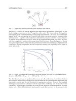
FIGURE 14.14
Oceans and clouds play an important part in the earth’s climate
system. How they will respond to increasing global
temperatures is not clear. Oceans may well add water vapor to
the atmosphere, which might promote warming by enhancing
the greenhouse effect. An increase in global cloudiness could
potentially enhance or reduce the warming produced by
increasing greenhouse gases.
ation from the earth than they emit upward. Low strat-
ified clouds, on the other hand, tend to promote a net
cooling effect. Composed mostly of water droplets, they
reflect much of the sun’s incoming energy, and, because
their tops are relatively warm, they radiate away much
of the infrared energy they receive from the earth. Satel-
lite data from the Earth Radiation Budget Experiment
confirm that, overall, clouds presently have a net cooling
effect on our planet, which means that, without clouds,
our atmosphere would be warmer.
Additional clouds in a warmer world would not
necessarily have a net cooling effect, however. Their
influence on the average surface air temperature would
depend on their extent and on whether low or high
clouds dominate the climate scene. Consequently, the
feedback from clouds could potentially enhance or
reduce the warming produced by increasing greenhouse
gases. Most models show that as the surface air warms,
there will be more convection, more convective-type
clouds, and an increase in cirrus clouds. This situation
would tend to provide a positive feedback on the cli-

mate system, and the effect of clouds on cooling the
earth would be diminished.
Some scientists speculate that an increase in tower-
ing cumuliform clouds, brought on by enhanced con-
vection, will promote another negative feedback on
global warming. They contend that as cumulus clouds
develop, much of their water vapor will condense and
fall to the surface as rain, leaving the upper part of the
clouds relatively dry. Additionally, sinking air filling the
space around the clouds produces warmer and dryer air
aloft. Less water vapor, they feel, will diminish the effect
of greenhouse warming. All modeling and observa-
tional studies, however, do not support these ideas, as
convection generally moistens rather than dries the
middle and upper troposphere.
In addition to the amount and distribution of
clouds, the way in which climate models calculate the
cloud’s optical properties (such as albedo) can have a
large influence on the model’s calculations. For exam-
ple, to illustrate the effect that cloud properties might
have on climate models, researchers at the British Mete-
orological Office altered the representation of clouds in
their model. Initially, the model projected a global tem-
perature rise of about 5°C, accompanying a doubling
of atmospheric CO
2
. However, when water clouds re-
placed ice clouds in the simulation, the projected tem-
perature rise was less than 2°C. It is no wonder, then,
that a study conducted with 14 climate models showed

good agreement on how the global climate would
respond if current values of CO
2
were doubled under
clear skies. But when clouds were incorporated into the
models, the models did not agree, and, in fact, varied
greatly over a wide range.
POSSIBLE CONSEQUENCES OF GLOBAL WARMING
Most climate experts feel that increasing levels of green-
house gases will, by the end of this century, cause the
earth to warm by between 1° and 3.5°C. Look back to
Fig. 14.3, p. 374, and observe that even if the warming
turns out to be 1°C, the earth will be warmer than at any
other time during the past 5000 years. A warming of
3.5°C would be equivalent to the rise in temperature
since the Younger-Dryas event. Climate models predict
that the warming should be greatest over the high
northern latitudes in winter with little warming over the
Arctic in summer. Overall, in winter, surface warming
should be greater over land areas than over the oceans.
Some climatic models predict that, if average
global temperatures increase by about 3°C, the jet
stream will weaken and global winds will shift from
their “normal” position. The added surface warmth will
enhance evaporation, which will lead to a greater world-
wide average precipitation. However, the shifting
upper-level winds might reduce precipitation over cer-
tain areas, which, in turn, would put added stress on
certain agricultural areas, especially when the models
predict that more precipitation will fall in winter over

higher latitudes. Several models indicate that precipita-
tion intensity should increase, suggesting a possibility
for more extreme rainfall events, such as floods and
severe droughts. If the planet warms, total rainfall must
increase to balance the increase in evaporation. But at
this point, climate models are unable to determine
exactly how global precipitation patterns will change.
In a warmer world, most of the precipitation might
fall as rain, even in the mountainous regions of eastern
and western North America, which might allow much
of the winter runoff to end up in the sea, rather than in
reservoirs that capture melting snow during the spring.
Other consequences of global warming might be a
rise in the sea level as alpine glaciers recede, polar ice
Carbon Dioxide, the Greenhouse Effect, and Recent Global Warming 389
Beware when you buy that ocean-front property. If the
ocean level rises 50 cm (about 1.6 ft) by the end of this
century as predicted, ocean shorelines along the east
coast of North America could retreat by 750 m, or
2460 ft.
melts, and the oceans expand as they slowly warm.
Presently, estimates are that by the year 2100 sea level
will rise about 50 cm (20 in.) from its present level.
Taking into account both lower and higher tempera-
ture projections, the rise may be as low as 15 cm or as
high as 95 cm. Rising ocean levels might have a damag-
ing influence on coastal ecosystems. In addition,
coastal groundwater supplies might become contami-
nated with saltwater.
Climate models predict that the warming should

be greater in northern regions (see Fig. 14.15). In the
high latitudes of the Northern Hemisphere, the dark
green boreal forests absorb up to three times as much
solar energy as the snow-covered tundra. Consequently,
the winter temperatures in subarctic regions are, on the
average, about 11.5°C (21°F) higher than they would be
without trees. If warming allows the boreal forests to
expand into the tundra, the forests may accelerate the
warming in that region. As the temperature rises,
organic matter in the soil should decompose at a faster
rate, adding more CO
2
to the air, which might accelerate
the warming even more. Moreover, trees that grow in a
climate zone defined by temperature may become espe-
cially hard hit as rising temperatures place them in an
inhospitable environment. In a weakened state, they
may become more susceptible to insects and disease.
390 Chapter 14 Climate Change
Earlier in this chapter we learned
that, during the last glacier period,
the climate around Greenland (and
probably other areas of the world)
underwent shifts, from ice-age tem-
peratures to much warmer conditions
in a matter of years. What could
bring about such large fluctuations in
temperature over such a short period
of time? It now appears that a vast
circulation of ocean water, known as

the conveyor belt, plays a major role
in the climate picture.
Figure 2 illustrates the movement
of the ocean conveyor belt, or
thermohaline circulation.* The
conveyor-like circulation begins in
the north Atlantic near Greenland
and Iceland, where salty surface
water is cooled through contact with
cold Arctic air masses. The cold,
dense water sinks and flows
southward through the deep Atlantic
Ocean, around Africa, and into the
Indian and Pacific Oceans. In the
North Atlantic, the sinking of cold
water draws warm water northward
from lower latitudes. As this water
flows northward, evaporation
increases the water’s salinity
(dissolved salt content) and density.
When this salty, dense water
reaches the far regions of the North
Atlantic, it gradually sinks to great
depths. This warm part of the
conveyor delivers an incredible
amount of tropical heat to the north-
ern Atlantic. During the winter, this
heat is transferred to the overlying
atmosphere, and evaporation moist-
ens the air. Strong westerly winds

then carry this warmth and moisture
into northern and western Europe,
where it causes winters to be much
warmer and wetter than one would
normally expect for this latitude.
Ocean sediment records along
with ice-core records from Green-
land suggest that the giant conveyor
belt has switched on and off during
the last glacial period. Such events
have apparently coincided with
rapid changes in climate. For exam-
ple, when the conveyor belt is
strong, winters in northern Europe
tend to be wet and relatively mild.
However, when the conveyor belt is
weak or stops altogether, winters in
northern Europe appear to turn
much colder. This switching from a
period of milder winters to one of
severe cold shows up many times in
the climate record. One such
event—the Younger-Dryas—illus-
trates how quickly climate can
change and how western and north-
ern Europe’s climate can cool within
a matter of decades, then quickly
return back to milder conditions.
Apparently, the mechanism that
switches the conveyor belt off is a

massive influx of freshwater. For
example, about 11,000 years ago
during the Younger-Dryas event,
freshwater from a huge glacial lake
began to flow down the St.
Lawrence River and into the North
Atlantic. This massive inflow of fresh-
water reduced the salinity (and,
hence, density) of the surface water
to the point that it stopped sinking.
The conveyor shut down for about
1000 years during which time
severe cold engulfed much of
northern Europe. The conveyor belt
started up again when the influx of
freshwater began to drain down the
Mississippi rather than into the
North Atlantic. It was during this
time that milder conditions returned
to northern Europe.
Will increasing levels of CO
2
have an effect on the conveyor belt?
Some climate models predict that as
THE OCEAN CONVEYOR BELT AND CLIMATE CHANGE
Focus on a Special Topic
*Thermohaline circulations are ocean
circulations produced by differences in
temperature and/or salinity. Changes in
ocean water temperature or salinity create

changes in water density.
Although most climate scientists believe that over
the twenty-first century the earth will warm at an
unprecedented rate (a process that might cause many
problems), they also recognize that increasing levels of
CO
2
in the atmosphere may have some positive conse-
quences. For example, some scientists contend that the
higher level of CO
2
will act as a “fertilizer” for some
plants, accelerating their growth. Increased plant
growth consumes more CO
2
, which might retard the
increasing rate of CO
2
in the environment.
Other scientists feel that the increased plant
growth might force some insects to eat more, resulting
in a net loss of vegetation. There is concern also that a
major increase in CO
2
might upset the balance of
nature, with some plant species becoming so dominant
that others are eliminated. In cold climates, where crops
are now grown only marginally, the warming effect may
actually increase crop yield, whereas in tropical areas,
where many developing nations are located, the warm-

ing may decrease crop yield.
Moreover, rising temperatures may alter the way
landmasses absorb and emit CO
2
. For example, temper-
atures over the Alaskan tundra have risen dramatically
during the past 35 years to the point where more frozen
soil melts in summer than it used to. During warmer
months, deep layers of decaying peat release CO
2
into
Carbon Dioxide, the Greenhouse Effect, and Recent Global Warming 391
CO
2
levels increase, more precipita-
tion will fall over the North Atlantic.
This situation reduces the density of
the sea water and slows down the
conveyor belt. In fact, if CO
2
levels
double, computer models predict
that the conveyor belt will slow by
about 30 percent. If CO
2
levels
quadruple, models predict that the
conveyor belt will stop and severe
cold will return to northern Europe,
even though global temperatures

will likely increase dramatically.
W
a
r
m
s
a
l
t
y
w
a
t
e
r
Sinking
water
Deep, cold salty current
FIGURE 2
The ocean conveyor belt. In the North Atlantic, cold salty water sinks, drawing warm water northward from lower latitudes. The warm water
provides warmth and moisture for the air above, which is then swept into northern Europe by westerly winds that keep the climate of that
region milder than one would normally expect. When the conveyor belt stops, winters apparently turn much colder over northern Europe.
the atmosphere. Until recently, this region absorbed
more CO
2
than it released. Now, however, much of the
tundra acts as a source for CO
2
.
The effect that increasing levels of CO

2
might
have on the upper atmosphere is not totally clear.
However, climate models suggest that while the lower
atmosphere (troposphere) steadily warms, the upper
atmosphere (stratosphere, mesosphere, and thermo-
sphere) will cool. The cooling is brought on by the
additional molecules of CO
2
(and other trace gases)
emitting more infrared radiation both upward and
downward.
IS THE WARMING REAL? Earlier in this chapter we
saw that, over the last hundred years or so, the average
global surface air temperature has risen by about 0.7°C
(1.2°F). Is this warming real? Certainly, the greenhouse
effect is real. We know from Chapter 2 that our world
without water vapor, CO
2
, and other greenhouse gases
would be about 33°C (59°F) colder than at present.
With an average surface temperature of about –18°C
(0°F), much of the planet would be uninhabitable. In
Chapter 2, we also learned that when the rate of
incoming solar energy balances the rate of outgoing
infrared energy from the earth’s surface and atmo-
sphere, the earth-atmosphere system is in a state of
radiative equilibrium. Increasing concentrations of
greenhouse gases can disturb this equilibrium and are,
therefore, referred to as radiative forcing agents. The

radiative forcing* provided by extra CO
2
and other
greenhouse gases increased over the past several cen-
turies. Consequently, most climate scientists contend
that some of the warming during this century is due to
increasing greenhouse gases, but the exact amount of
warming is uncertain.
In an attempt to find a signal that suggests that
greenhouse gases are altering earth’s climate, scientists
initially turned their attention to polar regions, where
the warming should be greater. Here, they examined ice
sheets (especially the west Antarctic ice sheet) to see if
shrinkage of the ice might be occurring. But in polar
regions, as elsewhere around the globe, rising tempera-
tures produce complex interactions among temper-
ature, precipitation, and wind patterns. Hence, it is now
believed that as temperatures rise in south polar re-
gions, more snow will fall in the warmer (but still cold)
air, causing snow and ice to build up over the continent
of Antarctica. Perhaps, this idea explains why high
mountain glaciers in the tropics and middle latitudes of
the Northern Hemisphere are shrinking at record rates,
whereas those in polar regions are not.
In the previous section, we learned that computer
models predict that, in a warmer world, global precipi-
tation should increase. A recent study of weather
records for the past century has found evidence that
392 Chapter 14 Climate Change
90N

70N
30N
10N
50N
30S
10S
50S
70S
90S
180 150W
–6 –4 –2 0 2 4 6 8
7531
Temperature Change, °C
–1–3–5
120W 90W 60W 30W 0 30E 60E 90E 120E 150E 180
FIGURE 14.15
Projected changes in surface air
temperature due to a doubling of
CO
2
and human-induced sulfide
emissions with an Atmospheric
Ocean General Circulation Model
(AOGCM). Notice that the great-
est warming is projected for the
northern polar latitudes. [After F.
B. Mitchell et al., “Transient
climate response to increasing
sulphate aerosols and greenhouse
gases,” Nature (1995) 376:

501–504.]
*Radiative forcing is interpreted as an increase (positive) or a decrease (neg-
ative) in net radiant energy observed over an area at the tropopause. All fac-
tors being equal, an increase in radiative forcing may induce surface warm-
ing, whereas a decrease may induce surface cooling.
precipitation across the United States has indeed
increased by about 10 percent, with most of the increase
occurring in winter. Also, the frequency of extreme
rainfall events (such as days with rainfall amounts
exceeding 2 in.) has increased by almost 10 percent dur-
ing the past century. Analyses of precipitation in other
countries shows similar trends.
There are a few scientists who contend that the
problem of global warming is overstated. They believe
that there are too many uncertainties in the climate
models to adequately represent the highly complex
atmosphere, especially with respect to clouds and
oceans. Some point to the fact that many climate mod-
els predict that, due to increasing levels of greenhouse
gases, average global temperatures should have already
risen by at least 1°C, instead of less than 1°C, as
observed. Others feel that the warming is statistical in
nature and falls within the earth’s natural variability of
climate change.
Critics of global warming point to the fact that,
even though the surface has warmed dramatically over
the past two decades, the overall troposphere has not.
Since 1979, satellite measurements indicate that, within
the troposphere, the air has warmed 0° to 0.2°C,
whereas surface stations during the same period show a

warming of 0.25°C to 0.4°C. If an enhanced atmo-
spheric greenhouse effect is in fact causing the surface
warming, why hasn’t the atmosphere warmed in tan-
dem? One answer may be that perhaps natural events,
such as the ocean warming during El Niño and the
cooling induced by large volcanic eruptions, may
account for part of the temperature differences. Also, it
could well be the case that the thinning of ozone in the
stratosphere may be partly responsible for a cooler
upper troposphere.
With levels of CO
2
increasing by more than 28 per-
cent over the past 100 years, why has the observed
increase in global temperature been so small? Some
researchers suggest that the large heat capacity of the
ocean is delaying the warming of the atmosphere. In
addition, other natural factors (such as changes in the
radiation output of the sun and volcanic eruptions that
inject large quantities of sulfur dioxide into the strato-
sphere) may be countering the warming. Recent find-
ings, however, indicate that human-related emissions of
sulfur, leading to sulfuric aerosols (plus human impact
on other aerosols), appear to be responsible for the cli-
mate response being smaller than one would have
expected from increasing levels of CO
2
and other green-
house gases.
Notice in Fig. 14.16 that, when the cooling effects

of sulfate aerosols and changes in the sun’s energy out-
put are added to the latest climate models along with
greenhouse gases, the predicted temperatures are very
close to those observed. Note also that when greenhouse
gases alone are put into the models (as was done in the
past), the predicted temperatures are considerably
higher than those observed.
Indeed, because the interactions between the earth
and its atmosphere are so complex, it is difficult to
unequivocally prove that the recent warming trend has
been due primarily to increasing concentrations of
greenhouse gases. The problem is that any human-
induced signal of climate change is superimposed on
a background of natural climatic variations (“noise”)
such as the El Niño–Southern Oscillation (ENSO) phe-
nomenon (discussed in Chapter 7). Moreover, in the
temperature observations it is difficult to separate a sig-
nal from the noise of natural climate variability.
The Intergovernmental Panel on Climate Change
(IPCC), a committee of over 2000 leading earth scien-
tists, considered the issues of climate change in a report
Carbon Dioxide, the Greenhouse Effect, and Recent Global Warming 393
Greenhouse gases alone
Greenhouse gases and aerosols
Greenhouse gases, aerosols, and solar radiation
Observed temperatures
1.2
1.0
0.8
0.6

0.4
0.2
0
–0.2
1860 1880 1900 1920 1940 1960 1980 2000
Year
Temperature Change, °C
FIGURE 14.16
Projected surface air temperature changes from different climate
models. Model input from greenhouse gases only is shown in yel-
low; input from greenhouse gases plus aerosols is shown in blue;
input from greenhouse gases, sulfate aerosols, and solar energy
changes is shown in red. The gray line shows observed surface
temperatures. The dashed line is the 1880–1999 mean
temperature. (Redrawn from “The Science of Climate Change”
by Tom M. L. Wigley, published by the Pew Center of Global Cli-
mate Change.)
published in 1990. Updated in 1992, and again in 1995,
the report concluded that:
■ Emissions resulting from human activities are sub-
stantially increasing the atmospheric concentrations
of the greenhouse gases carbon dioxide, methane,
and nitrous oxide.
■ Many greenhouse gases remain in the atmosphere for
a long time (decades to centuries in the case of carbon
dioxide and nitrous oxide); hence, such gases enhance
the greenhouse effect up to hundreds of years.
■ Global mean surface air temperature has increased
by between 0.3° to 0.6°C since the late nineteenth
century.

■ The cooling effect of sulfate aerosols resulting from
sulfur emissions may have offset a significant part of
the greenhouse warming during the past several
decades.
■ Carbon dioxide concentrations are likely to reach
500 parts per million by the year 2100.
■ Increasing levels of greenhouse gases are likely to
cause the global mean surface air temperature to
increase by between 1° and 3.5°C (with the best esti-
mate being 2°C) by the year 2100.
■ Global sea level has risen by between 10 and 25 cm
over the past 100 years, and much of the rise may be
related to the increase in global mean temperature.
■ Average sea level is expected to rise between 15 and
95 cm (with the best estimate being 50 cm) by the
year 2100.
■ Warmer global temperatures will lead to a more vig-
orous hydrological (water) cycle. This prediction
translates into prospects for more severe droughts
and/or floods in some places and less severe droughts
and/or floods in other places.
■ There are many uncertainties in climate predictions,
particularly with regard to the timing, magnitude,
and regional patterns of climate change.
■ There are uncertainties in the magnitude and pat-
terns of long-term natural climatic variability. Never-
theless, the balance of evidence suggests that there is a
discernible human influence on global climate.
But, in reality, how much influence does humanity
have on global climate? Earlier, we learned that over the

past 100 years or so, the earth’s average surface temper-
ature has risen by as much as 0.7°C. Will the climate
slowly continue to warm, or will it warm at an accel-
erated rate due to increasing concentrations of green-
house gases? Are we in a natural cycle where the
temperature will soon level off, then slowly drop? In
centuries to come, will the Northern Hemisphere enter
a cooler period as predicted by the Milankovitch cycles?
Certainly, climate has changed in the past, but how
much and how quickly will it change in the future?
Unfortunately, at present, we have no answers to these
important questions. However, as we learn more about
our complicated and imperfectly understood atmo-
sphere, we will gain better insight into what the future
may have in store for the climate of our globe.
Even though there is uncertainty about the rate
and patterns of future global warming, cutting down on
the emissions of greenhouse gases and pollutants could
have potentially positive benefits, such as reducing acid
rain, diminishing haze, and slowing stratospheric ozone
depletion. Even if the greenhouse warming proves to be
less than today’s consensus, these measures would cer-
tainly benefit humanity.
IN PERSPECTIVE As scientists debate the causes and
effects of global warming, modification of the earth’s
surface, taking place right now, could potentially influ-
ence the immediate climate of certain regions. For
example, studies show that about half the rainfall in the
Amazon River Basin is returned to the atmosphere
through evaporation and through transpiration from

the leaves of trees. Consequently, clearing large areas of
tropical rain forests in South America to create open
areas for farms and cattle ranges will most likely cause a
decrease in evaporative cooling. This decrease, in turn,
could lead to a warming in that area of at least several
degrees Celsius. In turn, the reflectivity of the deforested
area will change. Similar changes in albedo result from
the overgrazing and excessive cultivation of grasslands
in semi-arid regions, causing an increase in desert con-
ditions (a process known as desertification).
Currently, billions of acres of the world’s range and
cropland, along with the welfare of millions of people,
are affected by desertification. Annually, millions of
acres are reduced to a state of near or complete useless-
ness. The main cause is overgrazing, although overculti-
vation, poor irrigation practices, and deforestation also
play a role. The effect that these kinds of activities will
have on climate, as surface albedos increase and more
dust is swept into the air, is uncertain. (For a look at
how a modified surface influences the inhabitants of a
region in Africa, read the Focus section on p. 395.)
394 Chapter 14 Climate Change
Carbon Dioxide, the Greenhouse Effect, and Recent Global Warming 395
The Sahel is in North Africa, located
between about 14° and 18°N latitude
(see Fig. 3). Bounded on the north by
the dry Sahara and on the south by the
grasslands of the Sudan, the Sahel is a
semi-arid region of variable rainfall. Pre-
cipitation totals may exceed 50 cm (20

in.) in the southern portion while in the
north, rainfall is scanty. Yearly rainfall
amounts are also variable as a year
with adequate rainfall can be followed
by a dry one.
During the winter, the Sahel is dry,
but, as summer approaches, the
Intertropical Convergence Zone (ITCZ)
with its rain usually moves into the re-
gion. The inhabitants of the Sahel are
mostly nomadic people who migrate to
find grazing land for their cattle and
goats. In the early and middle 1960s,
adequate rainfall led to improved
pasture lands; herds grew larger and so
did the population. However, in 1968,
the annual rains did not reach as far
north as usual, marking the beginning
of a series of dry years and a severe
drought.
Rain fell in 1969, but the totals were
far below those of the favorable years
in the mid-1960s. The decrease in
rainfall, along with overgrazing, turned
thousands of square kilometers of past-
ure into barren wasteland. By 1973,
when the severe drought reached its cli-
max, rainfall totals were 50 percent of
the long-term average, and perhaps 50
percent of the cattle and goats had

died. The Sahara Desert had migrated
southward into the northern fringes of
the region, and a great famine had
taken the lives of more than 100,000
people. Many more of the
2 million or so inhabitants would have
perished had it not been for massive
outside aid.
Although low rainfall years have
been followed by wetter ones, relat-
ively dry conditions have persisted over
the region for the past 30 years or
so. The wetter years of the 1950s and
1960s appear to be due to the north-
ward displacement of the ITCZ. The
drier years, however, appear to be
more related to the intensity of rain that
falls during the so-called rainy season.
But what causes the lack of intense
rain? Some scientists feel that this
situation is due to a biogeophysical
feedback mechanism wherein less
rainfall and reduced vegetation cover
modify the surface and promote a
positive feedback relationship: Surface
changes act to reduce convective
activity, which in turn promotes or
reinforces the dry conditions. As an
example, when the vegetation is re-
moved from the surface (perhaps

through overgrazing or excessive
cultivation), the surface albedo (reflectiv-
ity) increases, and the surface tempera-
ture drops. But studies show that less
vegetation cover does not always result
in a higher albedo.
Since the mid-1970s the Sahara
Desert has not progressively migrated
southward into the Sahel. In fact, during
dry years, the desert does migrate south-
ward, but in wet years, it retreats. By the
same token, vegetation cover throughout
the Sahel is more extensive during the
wetter years. Consequently, desertifi-
cation is not presently overtaking the
Sahel, nor is the albedo of the region
showing much year-to-year change.
So the question remains: Why did
the Sahel go from a period of abundant
rainfall in the 1950s and early 1960s
to relatively dry conditions since then?
Was there a large change in the
surface albedo brought on by reduced
vegetation? Without adequate satellite
imagery during those years, it is impos-
sible to tell. Does this relatively dry spell
indicate a long-term fluctuation in
climate, or will the wetter years of the
1950s return? And if global temper-
atures rise into the next century, how

will precipitation patterns change? At
present, we have
no answers.
THE SAHEL—AN EXAMPLE OF CLIMATIC VARIABILITY AND HUMAN EXISTENCE
Focus on a Special Topic
FIGURE 3
The semi-arid Sahel of North Africa is bounded by the Sahara Desert to the north and grasslands to the south.
Sahara Desert
Sahel
Grasslands
Latitude (˚N)
30˚
20˚
10˚
10˚ W 0˚ 10˚ E
20˚ E 30˚ E
Sahara desert
Sahel
Tropical rain forest
Grasslands
Longitude
Summary
In this chapter, we considered some of the many ways
the earth’s climate can be changed. First, we saw that the
earth’s climate has undergone considerable change dur-
ing the geologic past. Some of the evidence for a chang-
ing climate comes from tree rings (dendrochronology),
chemical analysis of oxygen-isotopes in ice cores and
fossil shells, and geologic evidence left behind by ad-
vancing and retreating glaciers. The evidence from these

suggest that, throughout much of the geologic past
(before humanity arrived on the scene), the earth was
much warmer than it is today. There were cooler peri-
ods, however, during which glaciers advanced over large
sections of North America and Europe.
We examined some of the possible causes of cli-
mate change, noting that the problem is extremely com-
plex, as a change in one variable in the climate system
almost immediately changes other variables. One the-
ory suggests that the shifting of the continents, along
with volcanic activity and mountain-building, may
account for variations in climate that take place over
millions of years.
The Milankovitch theory proposes that alternating
glacial and interglacial episodes during the past 2 mil-
lion years are the result of small variations in the tilt of
the earth’s axis and in the geometry of the earth’s orbit
around the sun. Another theory suggests that certain
cooler periods in the geologic past may have been
caused by volcanic eruptions rich in sulfur. Still another
theory postulates that climatic variations on earth
might be due to variations in the sun’s energy output.
We examined how sophisticated climate models
project that the earth’s surface will continue to warm by
between 1°C and 3.5°C (with the best estimate being
2°C) by the year 2100, as increasing levels of CO
2
and
other trace gases enhance the atmospheric greenhouse
effect. We learned that more research is needed to

improve these climate models, especially in the area of
the representation of clouds, in order to better refine
these estimates.
Key Terms
The following terms are listed in the order they appear in
the text. Define each. Doing so will aid you in reviewing
the material covered in this chapter.
Questions for Review
1. What methods do scientists use to determine climate
conditions that have occurred in the past?
2. How does the overall climate of the world today com-
pare with the so-called normal climate throughout
earth’s history?
3. Explain how the changing climate influenced the for-
mation of the Bering land bridge.
4. What are some of the uncertainties in the temperature
record during the past 100 years?
5. How does today’s average global temperature compare
with the average temperature during the Little Ice Age?
6. What is the Younger-Dryas event? When did it occur?
7. When did the Little Ice Age occur? Did it occur during
a period of high sunspot activity? Explain.
8. What is a feedback mechanism? How does a positive
feedback mechanism differ from a negative feedback
mechanism?
9. Is the water vapor–temperature rise feedback positive
or negative? Explain.
10. How does the theory of plate tectonics account for cli-
mate change over periods of millions of years?
11. Describe the Milankovitch theory of climatic change

by explaining how each of the 3 cycles alters the
amount of solar energy reaching the earth.
12. Given the analysis of air bubbles trapped in polar ice
during the past 160,000 years (during colder glacial
periods), were CO
2
levels generally higher or lower
than they are presently?
13. What effect do tropospheric sulfate aerosols have on
daytime surface temperatures?
14. What effect do sulfur-rich volcanic eruptions have on
surface temperatures?
15. Explain how variations in the sun’s energy might
influence global climate.
396 Chapter 14 Climate Change
dendrochronology
Ice Age
interglacial period
Younger-Dryas (event)
Little Ice Age
water vapor–temperature
rise feedback
positive feedback
mechanism
snow-albedo feedback
negative feedback
mechanism
theory of plate tectonics
Milankovitch theory
eccentricity

precession
obliquity
sulfate aerosols
Maunder minimum
radiative forcing agents
desertification
16. Explain how the ocean’s conveyor belt circulation
works. How does the conveyor belt appear to influ-
ence the climate of northern Europe?
17. List some of the consequences that increasing levels of
CO
2
and other greenhouse gases might have on the
atmosphere and its inhabitants.
18. Most climate models predict that increasing levels of
CO
2
will cause the mean global surface temperature to
rise by as much as 3.5°C by the year 2100. In order for
this condition to occur, what other greenhouse gas
must also increase in concentration?
19. (a) Describe how clouds influence the climate system.
(b) Which clouds would tend to promote surface
cooling: high clouds or low clouds?
20. Even though CO
2
concentrations have risen dramati-
cally over the past 100 years, how do scientists explain
the fact that global temperatures have risen only
slightly?

Questions for Thought
and Exploration
1. Ice cores extracted from Greenland and Antarctica
have yielded valuable information on climate changes
during the past few hundred thousand years. What do
you feel might be some of the limitations in using ice
core information to evaluate past climate changes?
2. When glaciation was at a maximum (about 18,000
years ago), was global precipitation greater or less than
at present? Explain your reasoning.
3. Consider the following climate change scenario.
Warming global temperatures increase saturation
vapor pressures over the ocean. As more water evapo-
rates, increasing quantities of water vapor build up in
the troposphere. More clouds form as the water vapor
condenses. The clouds increase the albedo, resulting in
decreased amounts of solar radiation reaching the
earth’s surface. Is this scenario plausible? What type(s)
of feedback(s) is/are involved?
4. Are ice ages in the Northern Hemisphere more likely
when the tilt of the earth is at a maximum or a mini-
mum? Explain.
5. Are ice ages in the Northern Hemisphere more likely
when the sun is closest to the earth during summer or
during winter? Explain.
6. The oceans are a major sink of CO
2
. According to one
hypothesis, continued global warming will result in
less CO

2
being dissolved in the oceans. Under this sce-
nario, would you expect the earth to warm or to cool
further? Explain your reasoning.
7. Use the Atmospheric Chemistry/Temperature Trends
section of the Blue Skies CD-ROM to examine climate
model predictions of future temperatures around the
globe. Describe the simulated global temperature pat-
terns 60 and 90 years into the future. What are the
major differences?
8. Global Climate Change Data (l
.gov/trends/trends.htm): Compare graphs of temper-
ature trends for the Northern Hemisphere, the South-
ern Hemisphere, and the globe. Compare and contrast
these trends. Which hemisphere has a trend that is
most similar to the global trend?
9. Venus ( .html):
Study the climate of Venus. In what ways is it similar or
dissimilar to the Earth’s climate? Compare the green-
house effect on both planets. Explain why Venus has a
“runaway” greenhouse effect, while the Earth does not.
10. Paleoclimate ( />tion.html): What is known about past climates? How
does the climate change of the past 100 years compare
to climate changes that have occurred in the past?
When was the last glaciation? Do you think it could
happen again?
For additional readings, go to InfoTrac College Edition,
your online library, at:

Questions for Thought and Exploration 397

White and Colors
White Clouds and Scattered Light
Blue Skies and Hazy Days
Red Suns and Blue Moons
Twinkling, Twilight, and the Green Flash
The Mirage: Seeing Is Not Believing
Focus on an Observation:
The Fata Morgana
Halos, Sundogs, and Sun Pillars
Rainbows
Coronas and Cloud Iridescence
Focus on an Observation:
Glories and the Heiligenschein
Summary
Key Terms
Questions for Review
Questions for Thought and Exploration
Contents
T
he sky is clear, the weather cold, and the year, 1818. Near
Baffin Island in Canada, a ship with full sails enters unknown
waters. On board are the English brothers James and John Ross,
who are hoping to find the elusive “Northwest Passage,” the water-
way linking the Atlantic and Pacific oceans. On this morning,
however, their hopes would be dashed, for directly in front of the
vessel, blocking their path, is a huge towering mountain range. Dis-
appointed, they turn back and report that the Northwest Passage
does not exist. About seventy-five years later Admiral Perry met the
same barrier and called it “Crocker land.”

What type of treasures did this mountain conceal—gold, silver,
precious gems? The curiosity of explorers from all over the world had
been aroused. Speculation was the rule, until, in 1913, the Ameri-
can Museum of Natural History commissioned Donald MacMillan to
lead an expedition to solve the mystery of Crocker land. At first, the
journey was disappointing. Where Perry had seen mountains,
MacMillan saw only vast stretches of open water. Finally, ahead of
his ship was Crocker land, but it was more than two hundred miles
farther west from where Perry had encountered it. MacMillan sailed
on as far as possible. Then he dropped anchor and set out on foot
with a small crew of men.
As the team moved toward the mountains, the mountains seemed
to move away from them. If they stood still, the mountains stood
still; if they started walking, the mountains receded again. Puzzled,
they trekked onward over the glittering snow-fields until huge moun-
tains surrounded them on three sides. At last the riches of Crocker
land would be theirs. But in the next instant the sun disappeared
below the horizon and, as if by magic, the mountains dissolved into
the cold arctic twilight. Dumbfounded, the men looked around only
to see ice in all directions—not a mountain was in sight. There they
were, the victims of one of nature’s greatest practical jokes, for
Crocker land was a mirage.
Light, Color, and Atmospheric Optics
399
T
he sky is full of visual events. Optical illusions
(mirages) can appear as towering mountains or
wet roadways. In clear weather, the sky can appear blue,
while the horizon appears milky white. Sunrises and
sunsets can fill the sky with brilliant shades of pink, red,

orange, and purple. At night, the sky is black, except for
the light from the stars, planets, and the moon. The
moon’s size and color seem to vary during the night,
and the stars twinkle. To understand what we see in the
sky, we will take a closer look at sunlight, examining
how it interacts with the atmosphere to produce an
array of atmospheric visuals.
White and Colors
We know from Chapter 2 that nearly half of the solar
radiation that reaches the atmosphere is in the form
of visible light. As sunlight enters the atmosphere, it
is either absorbed, reflected, scattered, or transmitted
on through. How objects at the surface respond to
this energy depends on their general nature (color, den-
sity, composition) and the wavelength of light that
strikes them. How do we see? Why do we see various
colors? What kind of visual effects do we observe be-
cause of the interaction between light and matter? In
particular, what can we see when light interacts with our
atmosphere?
We perceive light because electromagnetic waves
stimulate antenna-like nerve endings in the retina of the
human eye. These antennae are of two types—rods and
cones. The rods respond to all wavelengths of visible
light and give us the ability to distinguish light from
dark. If people possessed rod-type receptors only, then
only black and white vision would be possible. The
cones respond to specific wavelengths of visible light.
The cones fire an impulse through the nervous system
to the brain, and we perceive this impulse as the sensa-

tion of color. (Color blindness is caused by missing
or malfunctioning cones.) Wavelengths of radiation
shorter than those of visible light do not stimulate color
vision in humans.
White light is perceived when all visible wave-
lengths strike the cones of the eye with nearly equal
intensity. Because the sun radiates almost half of its
energy as visible light, all visible wavelengths from the
midday sun reach the cones, and the sun usually ap-
pears white. A star that is cooler than our sun radiates
most of its energy at slightly longer wavelengths; there-
fore, it appears redder. On the other hand, a star much
hotter than our sun radiates more energy at shorter
wavelengths and thus appears bluer. A star whose tem-
perature is about the same as the sun’s appears white.
Objects that are not hot enough to produce radia-
tion at visible wavelengths can still have color. Everyday
objects we see as red are those that absorb all visible
radiation except red. The red light is reflected from the
object to our eyes. Blue objects have blue light returning
from them, since they absorb all visible wavelengths
except blue. Some surfaces absorb all visible wave-
lengths and reflect no light at all. Since no radiation
strikes the rods or cones, these surfaces appear black.
Therefore, when we see colors, we know that light must
be reaching our eyes.
White Clouds and Scattered Light
One exciting feature of the atmosphere can be experi-
enced when we watch the underside of a puffy, growing
cumulus cloud change color from white to dark gray or

black. When we see this change happen, our first
thought is usually, “It’s going to rain.” Why is the cloud
initially white? Why does it change color? To answer
these questions, let’s examine the concept of scattering.
When sunlight bounces off a surface at the same
angle at which it strikes the surface, we say that the light
is reflected, and call this phenomenon reflection. There
are various constituents of the atmosphere, however,
that tend to deflect sunlight from its path and send it out
in all directions. We know from Chapter 2 that radiation
reflected in this way is said to be scattered. (Scattered
light is also called diffuse light.) During the scattering
process, no energy is gained or lost and, therefore, no
temperature changes occur. In the atmosphere, scatter-
ing is usually caused by small objects, such as air mole-
cules, fine particles of dust, water molecules, and some
pollutants. Just as the ball in a pinball machine bounces
off the pins in many directions, so solar radiation is
knocked about by small particles in the atmosphere.
Typical cloud droplets are large enough to effec-
tively scatter all wavelengths of visible radiation more or
less equally. Clouds, even small ones, are optically thick,
meaning that very little unscattered light gets through
them. These same clouds are poor absorbers of sun-
light. Hence, when we look at a cloud, it appears white
because countless cloud droplets scatter all wavelengths
of visible sunlight in all directions (see Fig. 15.1).
As a cloud grows larger and taller, more sunlight is
reflected from it and less light can penetrate all the way
through it (see Fig. 15.2). In fact, relatively little light

penetrates a cloud whose thickness is 1000 m (3300 ft).
400 Chapter 15 Light, Color, and Atmospheric Optics