- Trang chủ >>
- Khoa Học Tự Nhiên >>
- Vật lý
The Lecture Notes in Physics Part 7 pot
Bạn đang xem bản rút gọn của tài liệu. Xem và tải ngay bản đầy đủ của tài liệu tại đây (243.19 KB, 21 trang )
116 V. Zeitlin
∂
t
u
J
+
0 −J
−3
−10
∂
a
u
J
=
v
0
. (4.32)
The eigenvalues of the matrix in the l.h.s. of (4.32) are μ
±
=±J
−
3
2
and the
corresponding left eigenvectors are
1 , ±J
−
3
2
. Hence, Riemann invariants are
w
±
= u ± 2J
−
1
2
and we have
∂
t
w
±
+ μ
±
∂
a
w
±
= v. (4.33)
Expressions of original variables in terms of w
±
are
u =
1
2
(w
+
+ w
−
), J =
16
(w
+
− w
−
)
2
> 0 ,μ
±
=±
w
+
− w
−
4
3
. (4.34)
In terms of the derivatives of the Riemann invariants r
±
= ∂
a
w
±
, we get
∂
t
r
±
+ μ
±
∂
a
r
±
+
∂μ
±
∂w
+
r
+
r
±
+
∂μ
±
∂w
−
r
−
r
±
= ∂
a
v = Q(a) − J , (4.35)
which may be rewritten using Lagrangian derivatives along the characteristics
d
dt
±
=
∂
t
+ μ
±
∂
a
as
dr
±
dt
±
+
∂μ
±
∂w
+
r
+
r
±
+
∂μ
±
∂w
−
r
−
r
±
= Q(a) − J . (4.36)
Wave breaking and shock formation correspond to r
±
→±∞in finite time.
In terms of new variables R
±
= e
λ
r
±
, with λ =
3
128
log
|
w
+
− w
−
|
, (4.35) may
be rewritten as
dR
±
dt
±
=−e
−λ
∂μ
±
∂w
±
R
2
±
+ e
λ
(
Q(a) − J
)
, (4.37)
where
∂μ
±
∂w
±
=
3
64
(w
+
− w
−
)
2
> 0.
The qualitative analysis of these generalized Ricatti equations shows that if initial
relative vorticity Q − J = ∂
a
v is sufficiently negative (anti-cyclonic), rotation does
not stop wave breaking, which is taking place for any initial conditions. However,
if the relative vorticity is positive (cyclonic case), as well as the derivatives of the
Riemann invariants at the initial moment, there is no breaking. An example of wave
breaking due to the geostrophic adjustment of the unbalanced jet is presented in
Fig. 4.2.
4 Lagrangian Dynamics of Fronts, Vortices and Waves 117
−2L −L 0 L 2L
0
Vmax
Vjet
Fig. 4.2 Wave breaking and shock formation (right panel) during adjustment of the unbalanced
jet (left panel, top to bottom: consecutive profiles of the free surface with time measured in f
−1
units). Length is measured in deformation radius units: L = R
d
=
gH
f
4.2.1.6 “Trapped Waves” in 1.5d RSW: Pulsating Density Fronts
The above-established supra-inertiality of the spectrum of the small perturbations
around a balanced 1.5d RSW front means the absence of trapped waves, and, hence,
the attainability of the adjusted state by evacuating the excess of energy via inertia-
gravity wave emission (eventually with shock formation). There exist, however, the
RSW fronts, where the wave emission is impossible. These are the lens-type con-
figurations with terminating profile of fluid height. Such RSW configurations are
used to model oceanic double density fronts, either outcropping or incropping, e.g.
Griffiths et al. [10]. In Lagrangian description (4.9) the evolution of a double RSW
front corresponds to positive h
I
terminating at x = x
±
. Adjustment of such fronts,
therefore, should proceed without outward IGW emission. An example of adjusted
front treated in literature is given in Fig. 4.3.
A family of exact unbalanced pulsating solutions is known for such fronts (Frei [9];
Rubino et al. [22]). Let us make the following ansatz:
X(x, t) = xχ(t), h
I
(x) =
h
0
2
1 −
x
2
L
2
,v
I
(x) = x, (4.38)
Fig. 4.3 An example of equilibrated double density front
118 V. Zeitlin
where h
0
,,L are constants. Plugging (4.38) into (4.9) and non-dimensionalizing
with the timescale f
−1
and the length-scale L gives the following ODE for χ:
¨χ + χ −
γ
χ
2
= μ, (4.39)
where γ is the Burger number
gh
0
f
2
L
2
and μ = 1 +
f
.
Integrating (4.39) once gives
˙χ
2
2
+ P(χ) = E, P(χ) =
χ
2
2
− μχ +
γ
χ
, (4.40)
where the integration constant E is expressed in terms of initial conditions χ(t = 0)
= 1, ˙χ(t = 0) = U:
E =
U
2
2
+
1
2
− μ + γ. (4.41)
Equation (4.40) may be integrated in elliptic functions. The “potential” P(χ) being
convex, the solution for χ is finite amplitude and oscillating with supra-inertial
frequency. The minimum of P corresponds to the front in geostrophic equilibrium
and constant χ = 1. Thus, the adjustment (initial-value) problem for double density
fronts will result, in general, in a pulsating solution, whereas relaxation to the steady
state is possible only due to viscous effects (shocks).
4.2.2 Axisymmetric Case
4.2.2.1 Governing Equations and Lagrangian Invariants
Axisymmetric RSW motion is described in cylindrical coordinates by fields depend-
ing on radial variable only. As in the rectilinear case, it is possible to reduce the
whole dynamics to a single PDE for a Lagrangian variable R(r, t), the distance to
the center of a “particle” (or rather a particle ring) initially situated at r.
We first rewrite the Eulerian RSW equations in cylindrical coordinates (r,θ) and
assume exact axial symmetry:
(∂
t
+ u
r
∂
r
)u
r
− u
θ
f +
u
θ
r
+ ∂
r
h = 0 ,
(∂
t
+ u
r
∂
r
)u
θ
+ u
r
f +
u
θ
r
= 0 , (4.42)
∂
t
h +
1
r
∂
r
(ru
r
h) = 0 .
Here u
r
, u
θ
are the radial and azimuthal components of velocity. Note that the
adjusted stationary state changes character as compared to the rectilinear case: it
4 Lagrangian Dynamics of Fronts, Vortices and Waves 119
verifies conditions of the cyclo-geostrophic balance and not of the purely geostrophic
one:
u
θ
f +
u
θ
r
= ∂
r
h, u
r
= 0. (4.43)
Multiplying the second equation in (4.42) by r, we recover the conservation of angu-
lar momentum:
(∂
t
+ u
r
∂
r
)
ru
θ
+ f
r
2
2
= 0 , (4.44)
which replaces the conservation of geostrophic momentum in the plane-parallel
case. Equation (4.42) can be rewritten using the Lagrangian coordinate R(r, t).
Integrating (4.44) gives
R(r, t) u
θ
(r, t) + f
R
2
(r, t)
2
= ru
θ I
(r) + f
r
2
2
≡ G(r), (4.45)
where u
θ I
is the initial azimuthal velocity profile. Using the above expression we
get
u
θ
f +
u
θ
R
=
1
R
G − f
R
2
2
f +
G
R
2
−
f
2
=
1
R
3
G
2
−
f
2
R
4
4
. (4.46)
The mass conservation is expressed by the following relation:
h(r, t) R(r, t) dR = h
I
(r) rdr. (4.47)
With the help of (4.46), (4.47) and the definition
˙
R(r, t) = u
r
(r, t), the radial
momentum equation becomes
¨
R +
f
2
4
R −
1
R
3
G
2
+
1
∂
r
R
∂
r
rh
I
R ∂
r
R
= 0 , (4.48)
to be solved with initial conditions R(r, 0) = r,
˙
R(r, 0) = u
r
I
. The stationary part
of this equation defines the adjusted, slow states. The fast motions are axisymmetric
IGW. Indeed, for small perturbations about the state of rest:
R(r, t) = r + φ(r, t), (4.49)
with |φ|r , h
I
(r) = 1 and u
θ I
(r) = 0, the following equation is obtained after
some algebra:
120 V. Zeitlin
¨
φ + f
2
φ −
∂
r
φ
r
− ∂
2
rr
φ +
φ
r
2
= 0 . (4.50)
If solutions are sought in the form φ(r, t) =
ˆ
φ(r) e
iωt
, (4.50) yields, after a change
of variables, the canonical equation for the Bessel functions. The familiar axisym-
metric wave solutions involving Bessel functions J
1
then follow:
φ(r, t) = CJ
1
(
ω
2
− f
2
r) e
iωt
+ c.c., (4.51)
where C is the wave amplitude.
The whole program of the previous section may be carried on as well in cylindri-
cal coordinates, with similar conclusions. We present below only the case of the
axisymmetric density fronts (Sutyrin and Zeitlin [23]).
4.2.2.2 Axisymmetric Density Fronts and Radial “pulson” solutions
We make the following ansatz in (4.48):
h
I
(r) =
h
0
2
1 −
r
2
L
2
, R(r, t) = rφ(t), u
θ I
(r) = r, = const. (4.52)
Then by non-dimensionalizing the system in the same way as for the rectilinear
fronts, introducing the Burger number γ , and denoting M =
1
2
+
f
we get
¨
φ +
φ
4
−
M
2
φ
3
−
γ
φ
3
= 0, (4.53)
to be solved with initial conditions φ(0) = 1,
˙
φ(0) = u
r
I
. A drastic simplification
of this equation is provided by the substitution φ
2
= χ which immediately gives the
equation of the harmonic oscillator with shifted equilibrium position:
¨χ + χ −4E = 0, E =
u
2
r
I
2
+
1
8
+
M
2
+ γ
2
> 0. (4.54)
The “radial pulson” solution (cf. Rubino et al. [21] for a derivation in Eulerian
framework) satisfies the initial conditions χ(0) = 1, ˙χ(0) = 2u
r
I
and is given by
χ(t) = 4E + (1 − 4E) cost + (2u
r
I
+ 1 −4E) sin t. (4.55)
The crucial difference between the radial and rectilinear pulson, thus, is that the for-
mer always has inertial frequency and thus represents nonlinear inertial oscillations,
while the latter is always supra-inertial.
4 Lagrangian Dynamics of Fronts, Vortices and Waves 121
4.3 Including Baroclinicity: 2-Layer 1.5d RSW
4.3.1 Plane-Parallel Case
4.3.1.1 Governing Equations and General Properties of the Model
To introduce the baroclinic effects in the dynamics in the simplest way we consider
the two-layer rotating shallow water model. We use the rigid lid upper boundary
condition and again consider for simplicity a flat bottom. In this case the equations
governing the motion of two superimposed rotating shallow-water layers of unper-
turbed depths H
1,2
, H
1
+H
2
= H and densities ρ
1,2
in Cartesian coordinates under
hypothesis of no dependence of y (straight two-layer fronts) are
∂
t
u
i
+ u
i
∂
x
u
i
− f v
1
+ ρ
−1
i
∂
x
π
i
= 0 , (4.56a)
∂
t
v
i
+ u
i
( f + ∂
x
v
i
) = 0 , (4.56b)
∂
t
h
i
+ ∂
x
((h
i
u
i
) = 0 , i = 1, 2 (4.56c)
π
1
+ g
(ρ
1
h
1
+ ρ
2
h
2
) = π
2
, (4.56d)
h
1
+ h
2
= 1, (4.56e)
where no sum over repeated index is understood, π
i
are the pressures in the layers,
g
=
ρ
2
−ρ
1
ρ
2
+ρ
1
g is the reduced gravity and h
i
are the variable layers depths. A sketch
of the 2-layer 1.5d RSW is presented in Fig. 4.4.
The Lagrangian invariants of equations (4.56a), (4.56b) and (4.56c) are potential
vorticities and geostrophic momenta in each layer:
Q
i
=
f + ∂
x
v
i
h
i
, M
i
= fx+∂
x
v
i
, i = 1, 2. (4.57)
For any solution of system (4.56a), (4.56b), (4.56c), (4.56d) and (4.56e), constraint
(4.56e) imposes that
x
v2(x,t)
u2(x,t)
.
g
Ω
ρ2
ρ1
h2(x,t)
v1(x,t)
(x,t)
u1
h1(x,t)
Fig. 4.4 Schematic representation of the 2-layer 1.5d RSW model
122 V. Zeitlin
∂
x
(h
1
u
1
+ h
2
u
2
) = 0. (4.58)
Hence, the barotropic across-front velocity is
U =
h
1
u
1
+ h
2
u
2
H
= U(t). (4.59)
Choosing the boundary condition of absence of the mass flux across the front sets
U = 0. The geostrophic equilibria are stationary solutions:
u
i
= 0,v
i
=
1
f ρ
i
∂
x
π
i
, i = 1, 2 ,π
2
= π
1
+ g(ρ
1
h
1
+ ρ
2
h
2
). (4.60)
The fast motions in the linear approximation are internal inertia-gravity waves prop-
agating along the interface between the layers. By linearizing about the rest state
h
1
= H
1
, h
2
= H
2
, u
1,2
= 0,v
1,2
= 0, the dispersion relation for the waves with
frequency ω and wavenumber k follows:
ω
2
(ω
2
− f
2
− c
2
e
k
2
) = 0 . (4.61)
Here c
2
e
= g
H
e
is the phase speed of the waves, H
e
=
(ρ
2
−ρ
1
)H
1
H
2
ρ
1
H
1
+ρ
2
H
2
is the equivalent
height for the baroclinic modes of the model. As in the one-layer model, conditions
for existence and uniqueness of the adjusted state can be obtained as conditions for
existence and uniqueness of solutions to the PV equations (LeSommer et al. [14]).
These equations can be combined to give two ordinary differential equations for the
depths of the layers:
g
f
h
1
− (Q
2
+rQ
1
) h
1
=−
(
− f (1 −r) + HQ
2
)
, (4.62a)
g
f
h
2
− (Q
2
+rQ
1
) h
2
=−
(
f (1 −r) +rH Q
1
)
, (4.62b)
where notation r = ρ
1
/ρ
2
for the density ratio of the layers has been introduced and
the prime denotes the x
- differentiation. An essential difference of these equations
from their one-layer counterpart is that the forcing terms at the r.h.s. are not constant.
They, nevertheless, may be analysed by the same method as in 1dRSW.
For an equation of the form h
− R(x) h =−S(x), the existence and uniqueness
of solutions are guaranteed if R and S have constant asymptotics at ±∞. Further-
more, the solution is positive if R and S are positive. Hence, for the initial states
with localized PV anomalies such that
Q
1
≥ 0 and Q
2
≥ (1 −r) f/H , (4.63)
the above equations have unique solutions h
1
and h
2
that are everywhere positive.
4 Lagrangian Dynamics of Fronts, Vortices and Waves 123
A crucial simplification of the rigid-lid 2-layer equations follows from the fact
the pressures π
i
may be eliminated from (4.56a), (4.56b) and (4.56c). Indeed by
using (4.58) and (4.56e) and (4.56d) we get, again under the hypothesis of zero
overall across-front mass flux:
∂π
1
∂x
=
h
1
ρ
1
+
h
2
ρ
2
−1
f (h
1
v
1
+ h
2
v
2
) −
∂
∂x
h
1
u
2
1
+ h
2
u
2
2
−
gh
2
ρ
2
∂
∂x
(
ρ
1
h
1
+ ρ
2
h
2
)
, (4.64)
∂π
2
∂x
=
h
1
ρ
1
+
h
2
ρ
2
−1
f (h
1
v
1
+ h
2
v
2
) −
∂
∂x
h
1
u
2
1
+ h
2
u
2
2
+
gh
1
ρ
1
∂
∂x
(
ρ
1
h
1
+ ρ
2
h
2
)
. (4.65)
One can use (4.64), (4.65) in order to reduce the system to four equations for four
independent variables u
2
, h
2
,v
2
and v
1
, i.e. lower (heavier)-layer variables plus
upper-layer jet velocity:
∂u
2
∂t
+ u
2
∂u
2
∂x
− f v
2
+
ρ
1
ρ
2
h
1
+ ρ
1
h
2
f (h
1
v
1
+ h
2
v
2
)
−
∂
∂x
h
1
u
2
1
+ h
2
u
2
2
+
g(ρ
2
− ρ
1
)
ρ
1
h
1
∂h
2
∂x
= 0, (4.66)
∂h
2
∂t
+ u
2
∂h
2
∂x
+ h
2
∂u
2
∂x
= 0, (4.67)
∂v
2
∂t
+ u
2
∂v
2
∂x
+ fu
2
= 0, (4.68)
∂v
1
∂t
+ u
2
∂v
1
∂x
+ (u
1
− u
2
)
∂v
1
∂x
+ fu
1
= 0, (4.69)
where
u
1
=
h
2
u
2
h
2
− H
, h
1
= H − h
2
. (4.70)
4.3.1.2 Lagrangian Approach to 2-Layer 1.5d RSW
We start from the system (4.66), (4.67), (4.68), (4.69) and (4.70), taken for sim-
plicity in the frequently used limit r → 1 and introduce the Lagrangian coordinate
124 V. Zeitlin
X(x, t) corresponding to the positions of the fluid particles in the lower layer. In
terms of displacements φ with respect to initial positions X(x, t) = x + φ(x, t).
The corresponding Lagrangian derivative is
d
dt
=
∂
∂t
+u
2
∂
∂x
. The dependence of the
height variable h
2
on the Lagrangian labels and transformation of its derivatives are
obtained via the mass conservation in the lower layer: h
2
I
dx = h
2
(X(x, t), t)dX.
The subscript 2 will be omitted in what follows. As in the one-layer case, (4.68)
expresses the conservation of the geostrophic momentum in the lower layer and
allows to eliminate v
2
in terms of φ and its initial value:
v
2
(x, t) + f φ(x, t) = v
2
I
(x). (4.71)
The 2-layer Lagrangian equations, thus, are
¨
X − f
1 −
h
H
v
2
I
− v
1
− f (X − x)
−
1
X
h
˙
X
2
H − h
+ g
1 −
h
H
1
X
h
= 0,
(4.72)
˙v
1
−
˙
X
1 −
h
H
v
1
X
− f
h
H
= 0, (4.73)
where h =
h
I
(x)
X
, prime and dot denote x- and t-differentiations, respectively, and
g
= g
ρ
2
−ρ
1
ρ
2
– the reduced gravity in the limit r → 1.
4.3.1.3 Symmetric Instability
A qualitatively new phenomena appearing in the dynamics of fronts due to the baro-
clinic effects is a specific symmetric instability, i.e. an instability developing without
perturbations in the front-wise direction. This instability is frequently called inertial,
the term “symmetric” being often reserved for its moist counterpart (e.g. Bennetts
and Hoskins [2]).
For simplicity, we will consider the particular case of the initial conditions in the
form of a barotropic jet with h
2
I
= H
2
= const., v
2
I
= v
1
I
= v
I
(x). By introducing
the notation α
1
=
H
1
H
,α
2
=
H
2
H
,α
1
+ α
2
= 1 we have in non-dimensional form:
¨
φ + φ
α
1
+ φ
1 + φ
+
α
1
+ φ
1 + φ
(v
1
− v
I
) −
α
2
1 + φ
˙
φ
2
α
1
+ φ
− γ
1
(1 + φ
)
4
φ
= 0 ,
(4.74)
˙v
1
−
1
α
1
+ φ
˙
φv
1
−
α
2
α
1
+ φ
1
˙
φ = 0, (4.75)
where = Ro =
V
fL
is the Rossby number based on the typical jet velocity V and
typical jet width L, γ = Bu =
g
Hα
1
α
2
f
2
L
2
is the Burger number.
4 Lagrangian Dynamics of Fronts, Vortices and Waves 125
Equations (4.74), (4.75) are to be solved with initial conditions φ(x, 0) = 0,
˙
φ(x, 0)
= u
2
I
,v
1
(x, 0) = v
I
. The initial jet v
1
= v
I
,φ= 0, if non-perturbed: u
I
= 0isa
solution.
System (4.74), (4.75) in the linear approximation gives
¨
φ + α
1
φ + α
1
ξ
1
− γφ
= 0 , (4.76)
˙
ξ
1
−
v
I
α
1
˙
φv
I
−
α
2
α
1
1
˙
φ = 0 , (4.77)
where we introduced v
1
− v
I
= ξ . Hence,
φ
+
˙
φ(1 + v
I
) − γ
˙
φ
= 0 . (4.78)
Using the variable ψ =
˙
φ, renormalizing x with
√
γ and looking for the solution
ψ ∝ e
iωt
, we get the quantum-mechanical Schrödinger equation:
∂
2
xx
ψ +(E − V(x))ψ = 0 (4.79)
for a particle having the energy E = ω
2
and moving in the potential V(x) = 1+v
I
.
It is worth noting that Burger number plays the role of the Planck constant squared.
It is known (e.g. Landau and Lifshits [13]) that in the case of quantum mechanical
potential well there are both propagating solutions corresponding to the continuous
spectrum ω
2
≥ 1 and trapped in the well, localized solutions corresponding to the
discrete spectrum Min(V (x)) < ω
2
< 1. As is easy to see, the potential well cor-
responds to the region of anticyclonic shear. Hence, the trapped modes are localized
there, oscillating at sub-inertial frequencies.
If the potential is deep enough (strong enough anticyclonic shear), non-oscillatory
unstable modes with ω
2
< 0 appear and therefore a specific instability arises. This is
the symmetric instability which is thus intricately related to the presence of trapped
modes inside the front. It should be noted that the known explicit solutions of
the Schrödinger equations for some potentials, e.g. cosh
−2
potential (e.g. Landau
and Lifshits [13]) may be used for analytical studies of symmetric instability. The
Lagrangian equations (4.74), (4.75) provide a convenient framework for studying
the nonlinear stage of this instability.
4.3.1.4 Equatorial 2-Layer 1.5d RSW in Lagrangian Variables
As in the one-layer case, the Lagrangian description may be also applied to the
equatorial zonal flows. The equatorial counterparts of (4.72), (4.73), with obvious
interchanges between the zonal (u) and meridional (v) components of velocity and
respective Lagrangian coordinates, are
126 V. Zeitlin
¨
Y + βYu
2
+
−βY
(
(1 − h)u
1
+ hu
2
)
−
h
1 − h
˙
Y
2
Y
+ g
(1 − h)h
Y
= 0 ,
(4.80)
˙u
1
−
1 +
h
1 − h
˙
Yu
1
Y
+ β
h
1 − h
Y
˙
Y = 0, (4.81)
where
u
2
− β
Y
2
2
= u
2
I
− β
y
2
2
, (4.82)
h =
h
I
Y
and ∂
Y
=
1
Y
∂
y
.
Introducing φ(y, t) = Y(y, t) − y, linearizing around the barotropic jet u
2
I
=
u
1
I
= u
I
and non-dimensionalizing as above with an obvious change for the fre-
quency scale: f → β L, we get the equatorial counterpart of (4.78):
φ
− βy(u
I
− α
2
y)
˙
φ − γ
˙
φ
= 0 . (4.83)
This is an equation for linear equatorial symmetric (inertial) instability (e.g.
Dunkerton [8]). Unlike the mid-latitude case, even a linear shear may lead to sym-
metric instability at the equator. In this case (4.83) after Fourier tranformation in t
and a shift of y gives a quantum-mechanical Schrödinger equation for the harmonic
oscillator with well-known solutions.
4.3.1.5 Relation to 1.5 RSW and Comments on the Pulson Solutions
A limit of strong disparity between the layers depths
h
H
→ 0 may be considered in
(4.72), (4.73). This gives to zeroth order in
h
H
a system of decoupled equations:
¨
X − f
v
2
I
− v
1
− f (X − x)
+ g
1
X
h
I
X
= 0, (4.84)
˙v
1
−
˙
X
X
v
1
= 0. (4.85)
We thus recover in the case of motionless upper layer, when v
1
= 0, the one-layer
RSW equation in Lagrangian form (4.64), with the replacement g → g
, which
provides both a (standard) justification of the one-layer reduced-gravity model and
a possibility to calculate baroclinic corrections to the one-layer RSW solutions. For
example, the pulsating front solution presented in Sect. 4.2 is a zero-order in
h
H
solution of (4.72), (4.73), but corrections will appear in the next orders, in particular
the non-zero velocity field v
1
in the thick upper layer. They may be calculated order
by order, which will be presented elsewhere. It is, however, clear that a nontrivial
signature of the pulson solutions in the upper layer will appear.
4 Lagrangian Dynamics of Fronts, Vortices and Waves 127
4.3.2 Axisymmetric Case
As in the one-layer case, the Lagrangian approach can also be developed in the
axisymmetric case. The two-layer rigid-lid RSW equations for axisymmetric con-
figurations are described by the equations in polar coordinates r,θ:
(∂
t
+ u
(i)
r
∂
r
)u
(i)
r
− u
(i)
θ
f +
u
(i)
θ
r
+ ∂
r
π
(i)
=0 , (4.86a)
(∂
t
+ u
(i)
r
∂
r
)u
(i)
θ
+ u
(i)
r
f +
u
(i)
θ
r
=0 , (4.86b)
∂
t
h
(i)
+
1
r
∂
r
(ru
(i)
r
h
(i)
) =0 , i = 1, 2, (4.86c)
π
(1)
+ g(ρ
1
h
1
+ ρ
2
h
2
) =π
(2)
, (4.86d)
h
(1)
+ h
(2)
= 1, (4.86e)
where u
(i)
r
and u
(i)
θ
, i = 1, 2 are radial and azimuthal components of the velocity,
respectively, in each layer. The analog of constraint (4.58) is
∂
r
(rh
(1)
u
(1)
r
+rh
(2)
u
(2)
r
) = 0. (4.87)
Hence
U =
rh
(1)
u
(1)
r
+rh
(2)
u
(2)
r
H
= U(t). (4.88)
Choosing the boundary condition of zero-radial mass flux across the vortex bound-
ary sets U = 0gives
u
(1)
r
=−
h
(1)
H − h
(2)
u
(2)
r
. (4.89)
The pressures π
(i)
, i = 1, 2 may be excluded, as in the rectilinear case, and we thus
arrive at the following system of equations for four independent variables u
2
, h
2
,v
2
and v
1
, which is the axisymmetric counterpart of (4.66), (4.67), (4.68) and (4.69):
∂u
2
∂t
+ u
2
∂u
2
∂r
−
f +
v
2
r
v
2
+
ρ
1
ρ
2
h
1
+ ρ
1
h
2
f +
v
1
r
(h
1
v
1
) +
f +
v
2
r
(h
2
v
2
) −
∂
∂r
r(h
1
u
2
1
+ h
2
u
2
2
)
+
g(ρ
2
− ρ
1
)
ρ
1
h
1
∂h
2
∂r
= 0, (4.90)
128 V. Zeitlin
∂h
2
∂t
+
∂
∂r
(
ru
2
h
2
)
= 0, (4.91)
∂v
2
∂t
+ u
2
∂v
2
∂r
+ u
2
f +
v
2
r
= 0, (4.92)
∂v
1
∂t
+ u
2
∂v
1
∂r
+ (u
1
− u
2
)
∂v
1
∂r
+
f +
v
2
r
u
1
= 0, (4.93)
where we switched back to the lower index notation for the layer number and
denoted u
r
≡ u, u
θ
≡ v.
A Lagrangian version of these equations may be easily written down along the
lines of the plane-parallel case using the Lagrangian mapping r → R(r, t),the
angular momentum conservation and the mass conservation h
2
RdR = h
I
rdr, with
similar applications and conclusions, which we will not present here. It should be
emphasized that centrifugal instability replaces the symmetric (inertial) instability
in the axisymmetric case.
4.4 Continuously Stratified Rectilinear Fronts
4.4.1 Lagrangian Approach in the Case of Continuous
Stratification
The hydrostatic primitive equations for a continuously stratified fluid with no depen-
dence on y (the “2.5-dimensional” case) read:
∂
t
u + u∂
x
u + w∂
z
u − f v + g∂
x
φ =0 , (4.94a)
∂
t
v +u∂
x
v +w∂
z
v +uf =0 , (4.94b)
∂
z
φ = g
θ
θ
r
, (4.94c)
∂
x
u + ∂
z
w =0 , (4.94d)
(∂
t
+ u∂
x
+ w∂
z
)θ =0 . (4.94e)
Here they are written in the atmospheric context using potential temperature θ and
the so-called pseudo-height vertical coordinate (Hoskins and Bretherton [12]), θ
r
is a normalization constant. For oceanic applications potential temperature should
be replaced by density and the sign in the hydrostatic relation (4.94c) should be
changed, z then becomes the ordinary geometric coordinate.
Potential vorticity (PV)
q = ( f + ∂
x
v) ∂
z
θ − ∂
z
v∂
x
θ (4.95)
is a Lagrangian invariant (∂
t
+u∂
x
+w∂
z
)q = 0. As usual for straight fronts, there
exist an additional Lagrangian invariant, the geostrophic momentum
4 Lagrangian Dynamics of Fronts, Vortices and Waves 129
M = v + fx, (4.96)
where x is understood in Lagrangian sense. The expression for the potential vorticity
in terms of M is
q = ( f + ∂
x
v) ∂
z
θ − ∂
z
v∂
x
θ =
∂(M,θ)
∂(x, z)
. (4.97)
The “slow” balanced motions are geostrophic and hydrostatic equilibria
u = w = 0, f v = g∂
x
φ, ∂
z
φ = g
θ
θ
r
, (4.98)
which are exact stationary solutions of (4.94a), (4.94b) and (4.94c) and obey the
thermal wind relation
f
∂ M
∂z
=
g
θ
r
∂θ
∂x
. (4.99)
A potential may be introduced for balanced states, such that
M = f
−1
∂
∂x
,θ=
θ
r
g
∂
∂z
. (4.100)
In fact, is an “extended” geopotential given as = φ + f
2
x
2
2
.
The fast motions are internal inertia gravity waves. Their dispersion relation may
be easily obtained in the case of linear background stratification θ
0
(z) =
N
2
g
θ
r
z by
linearization about the state of rest:
ω
2
= N
2
k
2
x
k
2
z
+ f
2
, (4.101)
where ω is wave frequency, k
x,z
are the wavenumber components in the horizontal
and vertical directions, respectively and N
2
= g
θ
0
(z)
θ
r
.
Lagrangian variables in the vertical plane X(x, z, t) and Z(x, z, t) are introduced as
positions at time t of the fluid particles initially found at (x, z). The incompressibil-
ity equation is written in the form of the volume conservation:
∂(X, Z)
∂(x, z)
= 1 , (4.102)
The primitive equations become
130 V. Zeitlin
¨
X + f
2
X +
∂(φ, Z)
∂(x, z)
= v
I
+ f
2
x , (4.103)
∂(X,φ)
∂(x, z)
= g
θ
I
θ
r
, (4.104)
and the potential vorticity is expressed as
q =
∂( fx+ v
I
,θ
I
)
∂(x, z)
. (4.105)
Elimination of φ by cross-differentiation gives
∂(X,
¨
X − f v
I
− f
2
x)
∂(x, z)
+
g
θ
0
∂(θ
I
, Z)
∂(x, z)
= 0, (4.106)
∂(X, Z)
∂(x, z)
= 1, (4.107)
and for the stationary adjusted state, we get
∂(X, −f v
I
− f
2
x)
∂(x, z)
+
g
θ
0
∂(θ
I
, Z)
∂(x, z)
= 0, (4.108)
∂(X, Z)
∂(x, z)
= 1. (4.109)
4.4.2 Existence and Uniqueness of the Adjusted State
in the Unbounded Domain
To study the adjusted states it is convenient to use the PV equation written in terms
of :
∂
2
∂ X
2
∂
2
∂ Z
2
−
∂
2
∂ X∂ Z
2
=
gf
θ
r
q , (4.110)
where PV in the r.h.s. is understood as a function of (X, Z). This is the Monge–
Ampère equation. The boundary conditions which we will use far from the frontal
zone are
θ
|
z→±∞
= θ
r
N
2
g
z, N = const.,
¯
X
x→±∞
= x. (4.111)
Although these are formally Neumann-type boundary conditions, it is easy to see
that they are equivalent to the condition that far enough from the origin has the
form
4 Lagrangian Dynamics of Fronts, Vortices and Waves 131
|
|X|,|Z|→∞
= f
2
X
2
2
+ N
2
Z
2
2
. (4.112)
This means that on some distant ellipse (which is a convex curve) f
2
X
2
2
+ N
2
Z
2
2
=
const., the function is constant, so the problem of finding the adjusted state is
reduced to the first (Dirichlet) boundary-value problem for the Monge–Ampère
equation. Existence of solution is guaranteed if the r.h.s., i.e. the PV, is continuous
and positive (Pogorelov [18]). Moreover, if the condition of convexity is added,
which is the case of (4.112), the solution is unique. Thus, for positive PV, condition
of absence of symmetric instability, the adjusted state exists and is unique in the
absence of boundaries. It is to be emphasized that the criterion is the same as for
fronts in 1- and 2-layer RSW.
An alternative Lagrangian formulation using the geostrophic and isentropic coor-
dinates (M,θ)as independent variables in the Monge–Ampère equation was exten-
sively used in the literature, in particular by Cullen and collaborators [5–7]. In
(M,θ)coordinates, the thermal wind relation takes the form:
f
∂ X
∂θ
=
g
θ
r
∂ Z
∂ M
. (4.113)
Hence a potential for the final positions of the fluid particles may be introduced:
X =
g
θ
r
∂
∂ M
, Z = f
∂
∂θ
. (4.114)
The Jacobian of the transformation from (x, z) to (X, Z) can be rewritten as
∂(X, Z)
∂(M,θ)
∂(M,θ)
∂(x, z)
= 1 , (4.115)
from which we can obtain, replacing X and Z by their expressions (4.114) the fol-
lowing Monge–Ampère equation for with a “potential pseudo-density” which is
the inverse of the PV at the r.h.s.:
∂
2
∂ M
2
∂
2
∂θ
2
−
∂
2
∂ M∂θ
2
=
θ
r
gf
1
q
. (4.116)
Assuming that fluid on the boundaries remains there, this equation has oblique
Neumann-type boundary conditions
∂
∂θ
(M
±
(s), θ
±
(s)) =
z
±
f
, (4.117a)
g
θ
r
∂
∂ M
, f
∂
∂θ
→
(
x(M,θ),z(M,θ)
)
as M →±∞, (4.117b)
132 V. Zeitlin
where (M
±
(s), θ
±
(s)) define the upper (z
+
= H) and lower boundaries (z
−
= 0)
in (M,θ) space, s is a coordinate along those boundaries, x and z are initial posi-
tions. The domain in (M,θ) space is generally not convex which may prevent the
existence of the smooth solutions of Monge–Ampère equation, although in general,
this latter may be solved by methods of the optimal transportation theory (Benamou
and Brenier [1]).
To illustrate the possible non-existence of the smooth solutions of the adjustment
problem and the advantages of the Lagrangian approach, we give below an explicitly
integrable example of zero PV in the vertically bounded domain (cf. Ou [15]).
We start with a flow in a slab between z = 0 and z = 1 (in non-dimensional
variables) with purely horizontal density gradients and no vertical shear in v:
θ
I
= θ
I
(x), v
I
= v
I
(x), (4.118)
and solve (4.109). The stationary part of the horizontal momentum equation
reduces to
∂ X
∂z
f (v
I
+ f ) +
∂ Z
∂z
gθ
I
θ
0
= 0 , (4.119)
where the prime denotes the x-derivative. Integration of (4.119) gives
X =
F(x)
f v
I
+ f
2
−
gθ
I
/θ
0
f v
I
+ f
2
Z , (4.120)
and from the incompressibility equation it follows that
Z
2
gθ
I
/θ
0
f v
I
+ f
2
− 2
F
f v
I
+ f
2
Z + 2(G(x) + z) = 0 . (4.121)
The functions F(x), G(x) are to be determined from the boundary conditions. For
the unit strip in the x, z-plane they are
Z(x, 0) = 0 , Z(x, 1) = 1 . (4.122)
Hence
X = x + A(x)
1
2
− Z
, A =
gθ
I
/θ
0
f v
I
+ f
2
, (4.123)
Z =
1
A
(x)
⎡
⎣
1 +
1
2
A
(x) −
1 +
1
2
A
(x)
2
− 2zA
(x)
⎤
⎦
, (4.124)
4 Lagrangian Dynamics of Fronts, Vortices and Waves 133
Fig. 4.5 The end-state of the evolution of the zero-PV state with initially vertical isentropic sur-
faces in the case of existence (left panel, no crossing of the isentropes) and non-existence (right
panel, crossing of the isentropes) of the adjusted state
which is the explicit solution for the adjusted state.
If a discontinuity forms, it forms at a boundary due to the elliptic character of the
problem, i.e. where ∂
x
X(x, 0) = 0or∂
x
X(x, 1) = 0. This will happen if
∂ X
∂x
(x, 0) = 1 ±
1
2
A
(x) = 0 , (4.125)
i.e. if
g
f θ
0
gθ
I
/θ
0
f + v
I
=±2 . (4.126)
The positions of isentropic surfaces and isotachs may be easily obtained from
knowing explicit final positions of the fluid particles (4.123), (4.124) and using the
Lagrangian conservation of θ and M. It may be thus shown (Plougonven and Zeitlin
[17]) that singularity corresponds to intersecting isentropes, as shown in Fig. 4.5 and
infinite gradients of v. We thus have a frontogenesis process, which in fact coincides
with the classical scenario of Hoskins and Bretherton [12], with the only difference
that in their example the parameters of the system were driven towards the singular
case by an adiabatic change due to external deformation field.
4.4.3 Trapped Modes and Symmetric Instability in Continuously
Stratified Case
The Lagrangian approach is also efficient for studying symmetric/inertial instability
in the continuously stratified case. For this, we consider (4.94a), (4.94b), (4.94c),
(4.94d) and (4.94e) taken between the flat top z = H and bottom z = 0. We rewrite
them in the form (4.107) and introduce the deviations of the particle positions from
the stationary balanced state:
X =
¯
X + χ, Z =
¯
Z + ζ, (4.127)
134 V. Zeitlin
so that
∂(
¯
X + χ, ¨χ)
∂(x, z)
−
∂(
¯
X + χ, fM
I
)
∂(x, z)
+
g
θ
r
∂(θ
I
,
¯
Z + ζ)
∂(x, z)
= 0 . (4.128)
It is more convenient to use as independent variables the positions of the particles in
the adjusted state (
¯
X,
¯
Z), rather than the initial positions (x, z). When this change of
variables is made in (4.128), two terms which express the thermal wind relation in
the adjusted state cancel out. Furthermore, it is convenient to express the gradients
of ¯v and θ in the adjusted state through the geopotential
¯
φ, making explicit use of
geostrophic and hydrostatic balances. Equation (4.128) then becomes
∂
2
∂t
2
+ f
2
+
∂
2
¯
φ
∂
¯
X
2
∂χ
∂
¯
Z
+
∂
2
¯
φ
∂
¯
X∂
¯
Z
−
∂χ
∂
¯
X
+
∂ζ
∂
¯
Z
−
∂
2
¯
φ
∂
¯
Z
2
∂ζ
∂
¯
X
+
∂(χ, ¨χ)
∂(
¯
X,
¯
Z)
= 0 .
(4.129)
The incompressibility condition gives
∂χ
∂
¯
X
+
∂ζ
∂
¯
Z
+
∂(χ,ζ)
∂(
¯
X,
¯
Z)
= 0 . (4.130)
We non-dimensionalize these equations in the context of perturbations of a balanced
jet by rescaling time by f
−1
, the horizontal displacements by U/f , where U is
typical transverse velocity which is small with respect to the typical jet velocity V ,
so U = δV , with δ 1. Typical horizontal and vertical length scales are L and H,
respectively. The scale of the vertical displacements is UH/fL, from the continuity
equation. We thus obtain
∂
2
∂t
2
+ 1 + Ro
∂
2
¯
φ
∂
¯
X
2
∂χ
∂
¯
Z
+ Ro
∂
2
¯
φ
∂
¯
X∂
¯
Z
−
∂χ
∂
¯
X
+
∂ζ
∂
¯
Z
− Bu
∂
2
¯
φ
∂
¯
Z
2
∂ζ
∂
¯
X
++δ Ro
∂(χ, ¨χ)
∂(
¯
X,
¯
Z)
= 0 , (4.131a)
∂χ
∂
¯
X
+
∂ζ
∂
¯
Z
+ δ Ro
∂(χ,ζ)
∂(
¯
X,
¯
Z)
= 0 , (4.131b)
where Ro = V/ fLis the Rossby number and Bu = N
2
H
2
/ f
2
L
2
is the Burger
number. We consider intense jets and presume Ro ∼ 1, Bu ∼ 1. We expand χ and
ζ in small parameter δ and obtain to leading order from (4.131b):
∂χ
(0)
∂
¯
X
+
∂ζ
(0)
∂
¯
Z
= 0 , (4.132)
4 Lagrangian Dynamics of Fronts, Vortices and Waves 135
Hence there exists a streamfunction ψ
(0)
such that
χ
(0)
=−
∂ψ
(0)
∂
¯
Z
,ζ
(0)
=
∂ψ
(0)
∂
¯
X
. (4.133)
Equation (4.131a) becomes
∂
2
∂t
2
+ 1 +
∂
2
¯
φ
∂
¯
X
2
∂
2
ψ
(0)
∂
¯
Z
2
−
∂
2
¯
φ
∂
¯
X∂
¯
Z
∂
2
ψ
(0)
∂
¯
X∂
¯
Z
+
∂
2
¯
φ
∂
¯
Z
2
∂
2
ψ
(0)
∂
¯
X
2
= 0 . (4.134)
The boundary conditions are zero vertical displacements of parcels at the top and
bottom boundaries. This implies that ψ
(0)
is constant on the boundaries. As there
is no overall displacement of the fluid layer in the
¯
X-direction, these constants are
equal; they can be both set to zero: ψ
(0)
(
¯
X, 0) = ψ
(0)
(
¯
X, 1) = 0. ψ
(0)
should also
remain bounded as
¯
X →±∞. Equation (4.134) closely resembles the homoge-
neous part of the Sawyer–Eliassen equation (e.g. Holton [11], p. 275) except for
the term with the double-time derivative, which makes (4.134) prognostic. In the
Sawyer–Eliassen equation, this term is absent because the fast time has been filtered
out by balanced scaling, making the equation diagnostic.
Like in the two-layer case above, we take the simplest example of a barotropic
jet. The non-dimensional geopotential describing a balanced jet is
¯
φ = (
¯
X) +
¯
Z
2
2
. (4.135)
The mean stratification, which we suppose constant, is given by the second deriva-
tive of the second term in this expression and the jet velocity is ¯v =
, where the
prime denotes the
¯
X-derivative
= ∂/∂
¯
X. If an unbalanced fast component is
added to (4.135), the equation for its evolution is (cf. (4.134)):
(1 +
+ ∂
2
tt
)∂
2
¯
Z
¯
Z
ψ
(0)
+ ∂
2
¯
X
¯
X
ψ
(0)
= 0 . (4.136)
It allows a separation of variables and results in a regular Sturm–Liouville problem
in the vertical results; given the boundary conditions, the vertical eigenfunctions are
sin(nπ
¯
Z). Hence the solutions are sought in the form:
ψ
(0)
(
¯
X,
¯
Z, t) =
n
sin(nπ
¯
Z)ψ
(0)
n
(
¯
X, t). (4.137)
We look for ψ
(0)
n
(
¯
X, t) with a time dependence of the form e
−iωt
and get a Sturm–
Liouville problem on ]−∞, +∞[). We denote by
ˆ
ψ
nω
(x) the horizontal eigenfunc-
tion with vertical wavenumber n and frequency ω. The equation for
ˆ
ψ
nω
(
¯
X) has the
form of Schrödinger equation of a particle in a well:
∂
2
¯
X
¯
X
ˆ
ψ
nω
− n
2
π
2
(1 +
− ω
2
)
ˆ
ψ
nω
= 0 . (4.138)
136 V. Zeitlin
The factor n
2
π
2
may be removed by rescaling
¯
X as S = nπ
¯
X:
∂
2
SS
ˆ
ψ
nω
− (1 +
(S/nπ) −ω
2
)
ˆ
ψ
nω
= 0 , (4.139)
where the “potential” is (1 +
(S/nπ))and the eigenvalues are ω
2
. For any given
profile of , the depth of the potential is always the same, but its width depends on
the vertical wavenumber n: the smaller the vertical scale of the waves, the wider the
potential.
The Schrödinger equation (4.139) has a continuous and a discrete spectrum of eigen-
values ω
2
. The potential (1 +
) tends to one as
¯
X →∞; hence, for a given n,we
have
• continuous spectrum of solutions with ω>1. This part of the spectrum is doubly
degenerate (two independent solutions for each eigenvalue ω) and corresponds to
leftward and rightward propagating IGW.
• discrete spectrum of solutions with subinertial frequencies:
Min(1 +
)<ω<1 . (4.140)
This part of the spectrum is nondegenerate, and consists of solutions exponen-
tially decaying outside the region where (1 +
− ω
2
)<0, and oscillating
inside that region: they are trapped in the anticyclonic part of the jet.
• For a jet with relative vorticity lower than −1(i.e. − f in dimensional variables),
modes with ω
2
< 0 arise in the trapped mode spectrum, yielding the symmetric
instability, like in the two-layer case.
4.5 Conclusions
Thus we have shown that Lagrangian variables represent an excellent tool for han-
dling dynamics of symmetric fronts (translational symmetry) and vortices (rota-
tional symmetry), both qualitatively and quantitatively. Although it is known that
relaxing the strict symmetry can lead to qualitatively new effects (cf., e.g. Griffiths
et al. [10]), such fundamental “symmetric” phenomena as singularity formation
(catastrophic adjustment) or nonlinear stage of symmetric instability are still ill-
understood. We believe that the mathematical framework developed in the previous
sections will allow to advance in their understanding.
References
1. Benamou, J D., Brenier, Y.: A computational fluid mechanics solution to the Monge–
Kantorovich mass transfer problem. Numer. Math. 84, 375–393 (2000). 132
2. Bennets, D.A., Hoskins, B.J.: Conditional symmetric instability – possible explanation for
frontal rainbands. Q. J. R. Meteorol. Soc. 105, 945–962 (1979). 124
3. Blumen, W.: Geostrophic adjustment. Rev. Geophys. Space Phys. 10, 485–528 (1972). 109