- Trang chủ >>
- Khoa Học Tự Nhiên >>
- Vật lý
Fundamentals Of Geophysical Fluid Dynamics Part 2 ppt
Bạn đang xem bản rút gọn của tài liệu. Xem và tải ngay bản đầy đủ của tài liệu tại đây (375.77 KB, 29 trang )
58 Fundamental Dynamics
x, u
X, U
y, v
Y, V
z, w
Z, W
Ω
t &
T &
rotating coordinatesstationary coordinates
Fig. 2.9. A rotating coordinate frame with coordinates, (X, Y, Z, T ), and a
non-rotating frame with coordinates, (x, y, z, t). The rotation vector is parallel
to the vertical axis, ΩΩΩ = Ω
ˆ
z.
=
D
Dt
r
= ∂
T
+ U∂
X
+ V ∂
Y
+ W ∂
Z
. (2.94)
∇∇∇
s
=
ˆ
x∂
x
+
ˆ
y∂
y
+
ˆ
z∂
z
= ∇∇∇
r
=
ˆ
X∂
X
+
ˆ
Y∂
Y
+
ˆ
Z∂
Z
. (2.95)
Similarly, the incompressible continuity equation in (2.38) preserves its
form,
∇∇∇
s
· u = ∇∇∇
r
· U = 0 , (2.96)
implying that material parcel volume elements are the same in each
frame, with dx = dX. The tracer equations in (2.38) also preserve their
form because of (2.94). The material acceleration transforms as
Du
Dt
s
=
D
Dt
[
ˆ
xu +
ˆ
yv +
ˆ
zw]
=
D
Dt
[
ˆ
X(U −ΩY ) +
ˆ
Y(V + ΩX) +
ˆ
ZW ]
=
DU
Dt
r
+ 2Ω
ˆ
Z ×U +
1
ρ
0
∇∇∇
r
P , (2.97)
with
P = −
ρ
0
Ω
2
2
(X
2
+ Y
2
) . (2.98)
2.4 Earth’s Rotation 59
The step from the first and second lines in (2.97) is an application of
(2.92). In the step to the third line, use is made of (2.94) and the
relations,
D
ˆ
X
Dt
= Ω
ˆ
Y,
D
ˆ
Y
Dt
= −Ω
ˆ
X,
D
ˆ
Z
Dt
= 0 , (2.99)
that describe how the orientation of the transformed coordinates ro-
tates. Since ∇∇∇
s
φ = ∇∇∇
r
φ by (2.95), the momentum equation in (2.38)
transforms into
DU
Dt
r
+ 2Ω
ˆ
Z ×U = −∇∇∇
r
φ +
P
ρ
0
−
ˆ
Z
gρ
ρ
0
+ F . (2.100)
After absorbing the incremental centrifugal force potential, P/ρ
0
, into
a redefined geopotential function, φ, then (2.100) has almost the same
mathematical form as the original non-rotating momentum equation, al-
beit in terms of its transformed variables, except for the addition of the
Coriolis force, −2ΩΩΩ × U. The Coriolis force has the effect of accelerat-
ing a rotating-frame horizontal parcel displacement in the horizontally
perpendicular direction (i.e., to the right when Ω > 0). This acceler-
ation is only an apparent force from the perspective of an observer in
the rotating frame, since it is absent in the inertial-frame momentum
balance.
Hereafter, the original notation (e.g., x) will also be used for rotating
coordinates, and the context will make it clear which reference frame
is being used. Alternative geometrical and heuristic discussions of this
transformation are in Pedlosky (Chap. 1.6, 1987), Gill (Chap. 4.5,
1982), and Cushman-Roisin (Chap. 2, 1994).
2.4.2 Geostrophic Balance
The Rossby number, Ro, is a non-dimensional scaling estimate for the
relative strengths of the advective and Coriolis forces:
u · ∇∇∇u
2ΩΩΩ × u
∼
V V /L
2ΩV
=
V
2ΩL
, (2.101)
or
Ro =
V
fL
, (2.102)
where f = 2Ω is the Coriolis frequency. In the ocean mesoscale eddies
and strong currents (e.g., the Gulf Stream) typically have V ≤ 0.5 m
s
−1
, L ≈ 50 km, and f ≈ 10
−4
s
−1
(∼ 2π day
−1
); thus, Ro ≤ 0.1.
60 Fundamental Dynamics
In the atmosphere the Jet Stream and synoptic storms typically have
V ≤ 50 m s
−1
, L ≈ 10
3
km, and f ≈ 10
−4
s
−1
; thus, Ro ≤ 0.5.
Therefore, large-scale motions have moderate or small Ro, hence strong
rotational influences on their dynamics. Motions on the planetary scale
have a larger L ∼ a and usually a smaller V , so their Ro values are even
smaller.
Assume as a starting model the rotating Primitive Equations with
the hydrostatic approximation (2.58). If t ∼ L/V ∼ 1/fRo, F ∼ RofV
(or smaller), and Ro 1, then the horizontal velocity is approximately
equivalent to the geostrophic velocity, u
g
= (u
g
, v
g
, 0), viz.,
u
h
≈ u
g
,
and the horizontal component of (2.100) becomes
fv
g
=
∂φ
∂x
, fu
g
= −
∂φ
∂y
, (2.103)
with errors O(Ro). This is called geostrophic balance, and it defines
the geostrophic velocity in terms of the pressure gradient and Coriolis
frequency. The accompanying vertical force balance is hydrostatic,
∂φ
∂z
= −g
ρ
ρ
o
= −g(1 −αθ) , (2.104)
expressed here as a notational hybrid of (2.33), (2.58) and (2.80) with
the simple equation of state,
ρ/ρ
o
= 1 −αθ .
Combining (2.103)-(2.104) yields
f
∂v
g
∂z
= gα
∂θ
∂x
, f
∂u
g
∂z
= −gα
∂θ
∂y
, (2.105)
called thermal-wind balance. Thermal-wind balance implies that the ver-
tical gradient of horizontal velocity (or vertical shear) is directed along
isotherms in a horizontal plane with a magnitude proportional to the
horizontal thermal gradient.
Geostrophic balance implies that the horizontal velocity, u
g
, is ap-
proximately along isolines of the geopotential function (i.e., isobars) in
horizontal planes. Comparing this with the incompressible velocity po-
tential representation (Sec. 2.2.1) shows that
ψ =
1
f
φ + O(Ro) ; (2.106)
2.4 Earth’s Rotation 61
i.e., the geopotential is a horizontal streamfunction whose isolines are
streamlines (Sec. 2.1.1). For constant f (i.e., the f-plane approxi-
mation), ∂
x
u
g
+ ∂
y
v
g
= 0 for a geostrophic flow; hence, δ
h
= 0 and
w = 0 at this order of approximation for an incompressible flow. So
there is no divergent potential as part of the geostrophic velocity, i.e.,
X = χ = 0 (Sec. 2.2.1). However, the dynamically consistent evo-
lution of a geostrophic flow does induce small but nonzero X, χ, and
w fields associated with an ageostrophic velocity component that is an
O(Ro) correction to the geostrophic flow, but the explanation for this is
deferred to the topic of quasigeostrophy in Chap. 4.
Now make a scaling analysis in which the magnitudes of various fields
are estimated in terms of the typical magnitudes of a few primary quan-
tities plus assumptions about what the dynamical balances are. The
way that it is done here is called geostrophic scaling. The primary scales
are assumed to be
u, v ∼ V , x, y ∼ L , z ∼ H , f ∼ f
0
. (2.107)
From these additional scaling estimates are derived,
T ∼
L
V
, p ∼ ρ
0
f
0
V L , ρ ∼
ρ
0
f
0
V L
gH
, (2.108)
by advection as the dominant rate for the time evolution, geostrophic
balance, and hydrostatic balance, respectively. For the vertical velocity,
the scaling estimate from 3D continuity is W ∼ V H/L. However, since
geostrophic balance has horizontal velocities that are approximately hor-
izontally non-divergent (i.e., ∇∇∇
h
·u
h
= 0), they cannot provide a balance
in continuity to a w with this magnitude. Therefore, the consistent w
scaling must be an order smaller in the expansion parameter, Ro, viz.,
W ∼ Ro
V H
L
=
V
2
H
f
0
L
2
. (2.109)
Similarly, by assuming that changes in f(y) are small on the horizontal
scale of interest (cf., (2.88)) so that they do not contribute to the leading-
order momentum balance (2.103), then
β =
df
dy
∼ Ro
f
0
L
=
V
L
2
. (2.110)
This condition for neglecting β can be recast, using β ∼ f
0
/a (with
a ≈ 6.4×10
6
m, Earth’s radius), as a statement that L/a = Ro 1, i.e.,
L is a sub-global scale. Finally, with geostrophic scaling the condition
62 Fundamental Dynamics
for validity of the hydrostatic approximation in the vertical momentum
equation can be shown to be
Ro
2
H
L
2
1 (2.111)
by an argument analogous to the non-rotating one in Sec. 2.3.4 (cf.,
(2.72)).
Equipped with these geostrophic scaling estimates, now reconsider the
basis for the oceanic rigid-lid approximation (Sec. 2.3.3). The approxi-
mation is based on the smallness of D
t
h compared to interior values of
w. The scalings are based on horizontal velocity, V , horizontal length,
L, vertical length, H, and Coriolis frequency, f, a geostrophic estimate
for the sea level fluctuation, h ∼ fV L/g, and the advective estimate,
D
t
∼ V/L. These combine to give D
t
h ∼ fV
2
/g. The geostrophic
estimate for w is (2.109). So the rigid lid approximation is accurate if
w
Dh
Dt
V
2
H
f
0
L
2
fV
2
g
R
2
e
L
2
, (2.112)
with
R
e
=
√
gH
f
. (2.113)
R
e
is called the external or barotropic deformation radius (cf., Chap.
4), and it is associated with the density jump across the oceanic free
surface (as opposed to the baroclinic deformation radii associated with
the interior stratification; cf., Chap. 5). For mid-ocean regions with H ≈
5000 m, R
e
has a magnitude of several 1000s km. This is much larger
than the characteristic horizontal scale, L, for most oceanic currents.
Geostrophic scaling analysis can also be used to determine the con-
ditions for consistently neglecting the horizontal component of the local
rotation vector, f
h
= 2Ω
e
cos[θ], compared to the local vertical compo-
nent, f = 2Ω
e
sin[θ] (Fig. 2.8). The Coriolis force in local Cartesian
coordinates on a rotating sphere is
2ΩΩΩ
e
× u = ˆx (f
h
w − fv) + ˆy f u − ˆz f
h
u . (2.114)
In the ˆx momentum equation, f
h
w is negligible compared to fv if
Ro
H
L
f
h
f
1 , (2.115)
2.4 Earth’s Rotation 63
based on the geostrophic scale estimates for v and w. In the ˆz momentum
equation, f
h
u is negligible compared to ∂
z
p/ρ
0
if
H
L
f
h
f
1 , (2.116)
based upon the geostrophic pressure scale, p ∼ ρ
0
fLV . In middle and
high latitudes, f
h
/f ≤ 1, but it becomes large near the Equator. So, for
a geostrophic flow with Ro ≤ O(1), with small aspect ratio, and away
from the Equator, the dynamical effect of the horizontal component of
the Coriolis frequency, f
h
, is negligible. Recall that thinness is also
the basis for consistent hydrostatic balance. For more isotropic motions
(e.g., in a turbulent Ekman boundary layer; Sec. 6.1) or flows very near
the Equator, where f f
h
since θ 1, the neglect of f
h
is not always
valid.
2.4.3 Inertial Oscillations
There is a special type of horizontally uniform solution of the rotating
Primitive Equations (either stably stratified or with uniform density). It
has no pressure or density variations around the resting state, no vertical
velocity, and no non-conservative effects:
δφ = δθ = w = F = Q = ∇∇∇
h
= 0 . (2.117)
The horizontal component of (2.100) implies
∂u
∂t
− fv = 0,
∂v
∂t
+ fu = 0 , (2.118)
and the other dynamical equations are satisfied trivially by (2.117). A
linear combination of the separate equations in (2.118) as ∂
t
(1st) + f ×
(2nd) yields the composite equation,
∂
2
u
∂t
+ f
2
u = 0 . (2.119)
This has a general solution,
u = u
0
cos[ft + λ
0
] . (2.120)
Here u
0
and λ
0
are amplitude and phase constants. From the first
equation in (2.118), the associated northward velocity is
v = −u
0
sin[ft + λ
0
] . (2.121)
64 Fundamental Dynamics
The solution (2.120)-(2.121) is called an inertial oscillation, with a pe-
riod P = 2π/f ≈ 1 day, varying from half a day at the poles to infinity
at the Equator. Its dynamics is somewhat similar to Foucault’s pendu-
lum that appears to a ground-based observer to precess with frequency f
as Earth rotates underneath it; but the analogy is not exact (Cushman-
Roisin, Sec. 2.5, 1994). Durran (1993) interprets an inertial oscillation
as a trajectory with constant absolute angular momentum about the
axis of rotation (cf., Sec. 3.3.2).
For such a solution, the streamlines are parallel, and they rotate
clockwise/counterclockwise with frequency |f | for f > 0/< 0 in the
northern/southern hemisphere when viewed from above. The associ-
ated streamfunction (Sec. 2.2.1) is
ψ(x, y, t) = −u
0
(x sin[ft + λ
0
] + y cos[ft + λ
0
]) . (2.122)
The trajectories are circles (going clockwise for f > 0) with a radius of
u
0
/f, often called inertial circles. This direction of rotary motion is also
called anticyclonic motion, meaning rotation in the opposite direction
from Earth’s rotation (i.e., with an angular frequency about
ˆ
z with the
opposite sign of f). Cyclonic motion is rotation with the same sign as
f. The same terminology is applied to flows with the opposite or same
sign, respectively, of the vertical vorticity, ζ
z
, relative to f (Chap. 3).
Since f ∼ Ω ≈ 10
−4
s
−1
, it is commonly true that f N in the atmo-
spheric troposphere and stratosphere and oceanic pycnocline. Inertial
oscillations are typically slower than buoyancy oscillations (Sec. 2.2.3),
but both are typically faster than the advective evolutionary rate, V/L,
for geostrophic winds and currents.
3
Barotropic and Vortex Dynamics
The ocean and atmosphere are full of vortices, i.e., locally recirculating
flows with approximately circular streamlines and trajectories. Most of-
ten the recirculation is in horizontal planes, perpendicular to the gravita-
tional acceleration and rotation vectors in the vertical direction. Vortices
are often referred to as coherent structures, connoting their nearly uni-
versal circular flow pattern, no matter what their size or intensity, and
their longevity in a Lagrangian coordinate frame that moves with the
larger-scale, ambient flow. Examples include winter cyclones, hurricanes,
tornadoes, dust devils, Gulf-Stream Rings, Meddies (a sub-mesoscale,
subsurface vortex, with L ∼ 10s km, in the North Atlantic whose core
water has chemical properties characteristic of the Mediterranean out-
flow into the Atlantic), plus many others without familiar names. A
coincidental simultaneous occurrence of well-formed vortices in Davis
Strait is shown in Fig. 3.1. The three oceanic anticyclonic vortices on
the southwestern side are made visible by the pattern of their advec-
tion of fragmentary sea ice, and the cyclonic atmospheric vortex to the
northeast is exposed by its pattern in a stratus cloud deck. Each vortex
type probably developed from an antecedent horizontal shear flow in its
respective medium.
Vortices are created by a nonlinear advective process of self-organization,
from an incoherent flow pattern into a coherent one, more local than
global. The antecedent conditions for vortex emergence, when it occurs,
can either be incoherent forcing and initial conditions or be a late-stage
outcome of the instability of a prevailing shear flow, from which fluctua-
tions extract energy and thereby amplify. This self-organizing behavior
conspicuously contrasts with the nonlinear advective dynamics of tur-
bulence. On average turbulence acts to change the flow patterns, to
increase their complexity (i.e., their incoherence), and to limit the time
65
66 Barotropic and Vortex Dynamics
Fig. 3.1. Oceanic and atmospheric vortices in Davis Strait (north of the
Labrador Sea, west of Greenland) during June 2002. Both vortex types are
mesoscale vortices with horizontal diameters of 10s-100s km. (Courtesy of
Jacques Descloirest, NASA Goddard Space Flight Center.)
over which the evolution is predictable. A central problem in GFD is how
these contrasting paradigms — coherent structures and turbulence —
can each have validity in nature. This chapter is an introduction to these
phenomena in the special situation of two-dimensional, or barotropic,
fluid dynamics.
3.1 Barotropic Equations
Consider two-dimensional (2D) dynamics, with ∂
z
= w = δρ = δθ = 0,
and purely vertical rotation with ΩΩΩ =
ˆ
z f/2. The governing momentum
and continuity equations under these conditions are
Du
Dt
− fv = −
∂φ
∂x
+ F
(x)
Dv
Dt
+ fu = −
∂φ
∂y
+ F
(y)
3.1 Barotropic Equations 67
∂u
∂x
+
∂v
∂y
= 0 , (3.1)
with
D
Dt
=
∂
∂t
+ u
∂
∂x
+ v
∂
∂y
.
These equations conserve the total kinetic energy,
KE =
1
2
dx dy u
2
, (3.2)
when F is zero and no energy flux occurs through the boundary:
d
dt
KE = 0 (3.3)
(cf., Sec. 2.1.4 for constant ρ and e in 2D). Equation (3.3) can be derived
by multiplying the momentum equation in (3.1) by u· , integrating over
the domain, and using continuity to show that there is no net energy
source or sink from advection and pressure force. The 2D incompress-
ibility relation implies that the velocity can be represented entirely in
terms of a streamfunction, ψ(x, y, t),
u = −
∂ψ
∂y
, v =
∂ψ
∂x
, (3.4)
since there is no divergence (cf., (2.24)). The vorticity (2.26) in this case
only has a vertical component, ζ = ζ
z
:
ζ =
∂v
∂x
−
∂u
∂y
= ∇
2
ψ . (3.5)
(In the present context, it is implicit that ∇∇∇ = ∇∇∇
h
.) There is no buoy-
ancy influence on the dynamics. This is an example of barotropic flow
using either of its common definitions, ∂
z
= 0 (sometimes enforced by
taking a depth average of a 3D flow) or ∇∇∇φ × ∇∇∇ρ = 0. (The opposite of
barotropic is baroclinic; Chap. 5). The consequence of these simplifying
assumptions is that the gravitational force plays no overt role in 2D fluid
dynamics, however much its influence may be implicit in the rationale
for why 2D flows are geophysically relevant (McWilliams, 1983).
3.1.1 Circulation
The circulation (defined in Sec. 2.1) has a strongly constrained time
evolution. This will be shown using an infinitesimal calculus. Consider
the time evolution of a line integral
C
A · dr, where A is an arbitrary
68 Barotropic and Vortex Dynamics
∆ t
∆ tv
1
∆ r
t
v
2
∆
C at t
C at t = t +
∆
r
2
r
1
1
r
r
2
r
Fig. 3.2. Schematic of circulation evolution for a material line that follows the
flow. C is the closed line at times, t and t
= t + ∆t. The location of two
neighboring points are r
1
and r
2
at time t, and they move with velocity v
1
and v
2
to r
1
and r
2
at time t
.
vector and C is a closed material curve (i.e., attached to the material
parcels along it). A small increment along the curve between two points
marked 1 and 2, ∆r = r
2
− r
1
, becomes ∆r
after a small interval, ∆t
(Fig. 3.2):
∆r
≡ r
2
− r
1
≈ (r
2
+ u
2
∆t) −(r
1
+ u
1
∆t)
= ∆r + (u
2
− u
1
)∆t , (3.6)
using a Taylor series expansion in time for the Lagrangian coordinate,
r(t). Thus,
∆r
− ∆r
∆t
≈ u
2
− u
1
≈
∂u
∂s
∆s = (∆r · ∇∇∇)u (3.7)
3.1 Barotropic Equations 69
for small ∆s = |∆r|, where s is arc length along C. As ∆t → 0, (3.7)
becomes
D
Dt
∆r = (∆r · ∇∇∇)u . (3.8)
This expresses the stretching and bending of ∆r through the tangential
and normal components of (∆r · ∇∇∇)u, respectively. Now divide C into
small line elements ∆r
i
to obtain
d
dt
C
A ·dr ≈
d
dt
i
A
i
· ∆r
i
=
i
DA
i
Dt
· ∆r
i
+ A
i
·
D∆r
i
Dt
=
i
DA
i
Dt
· ∆r
i
+ A
i
· (∆r
i
· ∇∇∇)u
(3.9)
for any vector field, A(r, t). The time derivative, d
t
, for the material
line integral as a whole is replaced by the substantial derivative, D
t
,
operating on each of the local elements, A
i
and ∆r
i
. As max
i
|∆r
i
| → 0,
(3.9) becomes
d
dt
C
A ·dr =
C
DA
Dt
· dr +
C
A ·(dr · ∇∇∇)u . (3.10)
When A = u, the last term vanishes because
C
u ·(dr · ∇∇∇)u =
C
u ·
∂u
∂s
ds
=
C
ds
∂
∂s
1
2
u
2
=
1
2
u
2
|
end
start
= 0 , (3.11)
since the start and end points are the same point for the closed curve,
C. Thus,
d
dt
C
u ·dr =
C
Du
Dt
· dr . (3.12)
The left-side integral operated upon by D
t
is called the circulation, C.
After substituting for the substantial derivative from the momentum
equations (3.1),
d
dt
C
u ·dr =
C
[−
ˆ
zf ×u −∇∇∇φ + F] ·dr . (3.13)
70 Barotropic and Vortex Dynamics
Two of the right-side terms are evaluated as
C
∇∇∇φ · dr =
C
∂φ
∂s
ds = 0 , (3.14)
and
−
C
ˆ
zf ×u ·dr = −
C
fu ·
ˆ
nds
=
C
f
∂ψ
∂s
ds
= −
C
ψ
∂f
∂s
ds , (3.15)
again using the fact that the integral of a derivative vanishes. So here
the form of Kelvin’s circulation theorem is
dC
dt
=
d
dt
C
u ·dr =
C
[−ψ∇∇∇f + F] ·dr . (3.16)
Circulation can only change due to non-conservative viscous or external
forces, or due to spatial variation in f, e.g., in the β-plane approximation
(Sec. 2.4). Insofar as the latter are minor effects, as is often true, then
circulation is preserved on all material circuits, no matter how much
the circuits move around and bend with the advecting flow field. This
strongly constrains the evolutionary possibilities for the flow, but the
constraint is expressed in an integral, Lagrangian form that is rarely
easy to interpret more prosaically.
Baroclinic Kelvin’s Theorem: As remarked after (3.5), the more
fundamental definition of baroclinic is ∇∇∇p × ∇∇∇ρ = 0. As a brief diver-
sion, consider Kelvin’s theorem for a fully 3D flow to see why ∇∇∇p×∇∇∇ρ is
germane to non-barotropic dynamics. For a fully compressible fluid,
the derivation of Kelvin’s circulation theorem includes the following
pressure-gradient term on its right side:
dC
dt
= −
C
1
ρ
∇∇∇p · ds + ···
= −
A
ˆ
n · ∇∇∇×
1
ρ
∇∇∇p
dA + ···
=
A
1
ρ
2
ˆ
n · ∇∇∇p × ∇∇∇ρ dA + ··· . (3.17)
The dots denote other contributions not considered here. The gradient
operator, ∇∇∇, here is fully 3D, A is the area of the 2D surface interior
3.1 Barotropic Equations 71
to the curve C, and
ˆ
n is the unit vector normal to this surface. With
the Boussinesq momentum approximation applied to circulation within
horizontal planes (i.e.,
ˆ
n =
ˆ
z),
dC
dt
=
A
ˆ
z
ρ
2
0
· ∇∇∇
h
p × ∇∇∇
h
ρ dx dy + ··· . (3.18)
Therefore, circulation is generated whenever ∇∇∇
h
p × ∇∇∇
h
ρ = 0, the usual
situation for 3D, stratified flows. But this will not happen if ρ = ρ
0
, or
ρ =
ρ(z), or {p = ˜p(x, y, t)ˆp(z), ρ = −(˜p/g) dˆp/dz, u
h
=
˜
u
n
ˆp }. The
first two of these circumstances are consistent with ∂u
h
/∂z = 0, a 2D
flow, while the third one is not. The third circumstance is often called an
equivalent barotropic flow, whose dynamics have a lot in common with
shallow-water flow (Chap. 4). For further discussion see Gill (p. 237-8,
1982).
3.1.2 Vorticity and Potential Vorticity
The vorticity equation is derived by taking the curl, (
ˆ
z · ∇∇∇
h
×) , of the
momentum equations in (3.1). Now examine in turn each term that
results from this operation. An arrow indicates the change in a term
coming from the momentum equation after applying the curl:
∂u
∂t
−→ −
∂
2
u
∂y∂t
+
∂
2
v
∂x∂t
=
∂ζ
∂t
; (3.19)
(u ·∇)u −→ −
∂
∂y
u
∂u
∂x
+ v
∂u
∂y
+
∂
∂x
u
∂v
∂x
+ v
∂v
∂y
= u
∂
2
v
∂x
2
−
∂
2
u
∂y∂x
+ v
∂
2
v
∂y∂x
−
∂
2
u
∂y
2
−
∂u
∂y
∂u
∂x
+
∂v
∂y
+
∂v
∂x
∂u
∂x
+
∂v
∂y
= u · ∇∇∇ζ , (3.20)
using the 2D continuity relation in (3.1);
∇∇∇φ −→ −
∂
∂y
∂φ
∂x
+
∂
∂x
∂φ
∂y
= 0 ; (3.21)
f
ˆ
z ×u −→ −
∂
∂y
(−fv) +
∂
∂x
(fu)
= f
∂u
∂x
+
∂v
∂y
+ u
∂f
∂x
+ v
∂f
∂y
72 Barotropic and Vortex Dynamics
= u · ∇∇∇f ; (3.22)
and
F −→ −
∂F
x
∂y
+
∂F
y
∂x
= F . (3.23)
The result is
Dζ
Dt
= −u · ∇∇∇f + F . (3.24)
The vorticity only changes following a parcel because of a viscous or
external force curl, F, or spatial variation in f. Notice the similarity
with Kelvin’s theorem (3.16). This is to be expected because, as derived
in Sec. 2.1,
C
u ·dr =
A
ζ dx dy . (3.25)
Equation (3.24) is a local differential relation, rather than an integral
relation, but since (3.16) applies to all possible material curves, both
relations cover the entire 2D domain.
Advection Operator: Using (3.4) the advection operator can be rewrit-
ten as
u · ∇∇∇A = u
∂A
∂x
+ v
∂A
∂y
= −
∂ψ
∂y
∂A
∂x
+
∂ψ
∂x
∂A
∂y
= J[ψ, A] (3.26)
for any advected field, A. J is called the Jacobian operator, and it is
the approximate form for advection in flows dominated by ψ (cf., Sec.
2.2.1), even in 3D.
Potential Vorticity: Since ∂
t
f = 0, (3.24) can be rewritten as
Dq
Dt
= F , (3.27)
with the potential vorticity defined by
q = f + ζ . (3.28)
When F = 0 (conservative flow), q is a parcel invariant; i.e., D
t
q = 0
for all parcels in the domain. This implies that a conservative flow can
3.1 Barotropic Equations 73
only rearrange the spatial distribution of q(x) without changing any of
its aggregate (or integral) properties; e.g.,
d
dt
dx dy q
n
= 0 (3.29)
for any value of n as long as there is no potential-vorticity flux at the
boundary, qu ·
ˆ
n = 0.
A Univariate Dynamical System: Equations (3.24) or (3.27), with
(3.5) and/or (3.28), comprise a partial differential equation system with
ψ as the only dependent variable (assuming that f is known and F can
be expressed in terms of the flow) because φ does not appear in the
potential vorticity equation, in contrast to the momentum-continuity
formulation (3.1). For example, with f = f
0
and F = 0, (3.24) can be
written entirely in terms of ψ as
∇
2
∂ψ
∂t
+ J[ψ, ∇
2
ψ] = 0 . (3.30)
Equation (3.30) is often called the barotropic vorticity equation since it
has no contributions from vertical shear or any other vertical gradients.
Rossby Waves: As an alternative to (3.30) when f = f(y) = f
0
+
β
0
(y − y
0
) (i.e., the β-plane approximation (2.88)) and advection is
neglected (i.e., the flow is linearized about a resting state), (3.24) or
(3.28) becomes
∇
2
∂ψ
∂t
+ β
0
∂ψ
∂x
= 0 . (3.31)
In an unbounded domain this equation has normal-mode solutions with
eigenmodes,
ψ = Real
ψ
0
e
i(kx+y−ωt)
, (3.32)
for an arbitrary amplitude constant, ψ
0
(with the understanding that
only the real part of ψ is physically meaningful) and eigenvalues (eigen-
frequencies),
ω = −
β
0
k
k
2
+
2
. (3.33)
This can be verified as a solution by substitution into (3.31). The type
of relation (3.33), between the eigenfrequency and the wavenumbers
and environmental parameters (here β
0
), is called a dispersion relation,
and it is a usual element for wave and instability solutions (Chap. 4).
74 Barotropic and Vortex Dynamics
These particular eigenmodes are westward-propagating (i.e., ω/k < 0),
barotropic Rossby waves. (Secs. 4.6-4.7 have more analyses.)
3.1.3 Divergence and Diagnostic Force Balance
The divergence equation is derived by operating on the momentum equa-
tions in (3.1) with (∇∇∇ ·) . Again examine the effect of this operation on
each term:
∂u
∂t
−→
∂
∂x
∂u
∂t
+
∂
∂y
∂v
∂t
= 0 ; (3.34)
(u · ∇∇∇)u −→
∂
∂x
u
∂u
∂x
+ v
∂u
∂y
+
∂
∂y
u
∂v
∂x
+ v
∂v
∂y
= −2
∂u
∂x
∂v
∂y
−
∂u
∂y
∂v
∂x
= −2J
∂ψ
∂x
,
∂ψ
∂y
; (3.35)
−∇∇∇φ −→ −∇
2
φ ; (3.36)
f
ˆ
z ×u −→
∂
∂x
(−fv) +
∂
∂y
(fu) = −∇∇∇·(f ∇∇∇ψ) ; (3.37)
and
F −→ ∇∇∇· F . (3.38)
The result is
∇
2
φ = ∇∇∇· (f ∇∇∇ψ) + 2J
∂ψ
∂x
,
∂ψ
∂y
+ ∇∇∇· F . (3.39)
This relation allows φ to be calculated diagnostically from ψ and F,
whereas, as explained near (3.30), ψ can be prognostically solved for
without knowing φ. The partial differential equation system (3.27) and
(3.39) is fully equivalent to the primitive variable form (3.1), given con-
sistent boundary and initial conditions. The former equation pair is a
system that has only a single time derivative. Therefore, it is a first-
order system that needs only a single field (e.g., ψ(x, 0)) as the initial
condition, whereas an incautious inspection of (3.1), by counting time
derivatives, might wrongly conclude that the system is second order,
requiring two independent fields as an initial condition. The latter mis-
take results from overlooking the consequences of the continuity equation
that relates the separate time derivatives, ∂
t
u and ∂
t
v. This mistake is
3.1 Barotropic Equations 75
avoided for the univariate system because the continuity constraint is
implicit in the use of ψ as the prognostic variable.
After neglecting ∇∇∇·F and using the following scaling estimates,
u ∼ V, x ∼ L, f ∼ f
0
,
ψ ∼ V L, φ ∼ f
0
V L, β =
df
dy
∼ Ro
f
0
L
, (3.40)
for Ro 1, (3.39) becomes
∇
2
φ = f
0
∇
2
ψ[ 1 + O(Ro) ] =⇒ φ ≈ f
0
ψ . (3.41)
This is the geostrophic balance relation (2.106). For general f and Ro,
the 2D divergence equation is
∇
2
φ = ∇∇∇· (f ∇∇∇ψ) + 2J
∂ψ
∂x
,
∂ψ
∂y
, (3.42)
again neglecting ∇∇∇·F.
This is called the gradient-wind balance relation. Equation (3.42) is
an exact relation for conservative 2D motions, but also often is a highly
accurate approximation for 3D motions with Ro ≤ O(1) and compati-
ble initial conditions and forcing. In comparison geostrophic balance is
accurate only if Ro 1. When the flow evolution satisfies a diagnos-
tic relation like (3.41) or (3.42), it is said to have a balanced dynamics
and, by implication, exhibits fewer temporal degrees of freedom than
allowed by the more general dynamics. Most large-scale flow evolution
is well balanced, but inertial oscillations and internal gravity waves are
not balanced (cf., Chaps. 2 and 4). Accurate numerical weather fore-
casts require that the initial conditions of the time integration be well
balanced, or the evolution will be erroneously oscillatory compared to
nature.
3.1.4 Stationary, Inviscid Flows
Zonal Flow: A parallel flow, such as the zonal flow,
u(x, t) = U(y)
ˆ
x , (3.43)
is a steady flow when F = 0 (e.g., when ν = 0). This is called an
inviscid stationary state, i.e., a non-evolving solution of (3.1) and (3.28)
for which the advection operator is trivial. On the f -plane a stationary
parallel flow can have an arbitrary orientation, but on the β-plane, with
76 Barotropic and Vortex Dynamics
f = f (y), only a zonal flow (3.43) is a stationary solution. This flow
configuration makes the advective potential-vorticity tendency vanish,
∂q
∂t
= − J[ψ, q] = − J
−
y
U(y
) dy
, f(y) −
dU
dy
(y)
= 0 ,
because the Jacobian operator vanishes if each of its arguments is a
function of a single variable, here y. In a zonal flow, all other flow
quantities (e.g., ψ, φ, ζ, q) are functions only of the coordinate y.
Vortex Flow: A simple example of a vortex solution for 2D, conserva-
tive, uniformly rotating (i.e., f = f
0
) dynamics is an axisymmetric flow
where ψ(x, y, t) = ψ(r), and r = [(x − x
0
)
2
+ (y −y
0
)
2
]
1/2
is the radial
distance from the vortex center at (x
0
, y
0
). This too is a stationary state
since in (3.24)-(3.26), J[ψ(r), ζ(r)] = 0 (see (3.75) for the definition of J
in cylindrical coordinates). The most common vortex radial shape is a
monopole vortex (Fig. 3.3). It has a monotonic decay in ψ as r increases
away from the extremum at the origin (ignoring a possible far-field be-
havior of ψ ∝ log[r]; see (3.50) below). An axisymmetric solution is
most compactly represented in cylindrical coordinates, (r, θ), that are
related to the Cartesian coordinates, (x, y), by
x = x
0
+ r cosθ, y = y
0
+ r sinθ . (3.44)
The solution has corresponding cylindrical-coordinate velocity compo-
nents, (U, V ), related to the Cartesian components by
u = Ucos θ −V sinθ, v = Usin θ + V cos θ . (3.45)
Thus, for an axisymmetric vortex,
u = U =
ˆ
z × ∇∇∇ψ −→ V =
∂ψ
∂r
, U = 0
ζ =
ˆ
z · ∇∇∇×u −→ ζ =
1
r
∂
∂r
[rV ] . (3.46)
A compact monopole vortex — whose vorticity, ζ(r), is restricted to
a finite core region (i.e., ζ = 0 for all r ≥ r
∗
) — has a nearly universal
structure to its velocity in the far-field region well away from its cen-
ter. Integrating the last relation in (3.46) with the boundary condition
V (0) = 0 (i.e., there can be no azimuthal velocity at the origin where
the azimuthal direction is undefined) yields
V (r) =
1
r
r
0
ζ(r
)r
dr
. (3.47)
3.1 Barotropic Equations 77
r
Ψ
V
ζ
ζ
anticyclonic monopole vortex (f > 0)
r
r
r
"bare"
"shielded"
or
Fig. 3.3. An axisymmetric anticyclonic monopole vortex (when f
0
> 0). (Left)
Typical radial profiles for ψ and V . (Right) Typical radial profiles for ζ,
showing either a monotonic decay (“bare”) or an additional outer annulus of
opposite-sign vorticity (“shielded”).
For r ≥ r
∗
, this implies that
V (r) =
C
2πr
. (3.48)
The associated far-field circulation, C, is
C(r) =
r≥r
∗
u ·dr
=
2π
0
V (r)r dθ
= 2πrV (r)
= 2π
r
∗
0
ζ(r
)r
dr
. (3.49)
C(r) is independent of r in the far-field; i.e., the vortex has constant
circulation around all integration circuits, C, that lie entirely outside r
∗
.
78 Barotropic and Vortex Dynamics
Also,
∂ψ
∂r
= V
⇒ ψ =
r
0
V dr
+ ψ
0
⇒ ψ ∼ ψ
0
as r → 0
⇒ ψ ∼
C
2π
ln r as r → ∞ . (3.50)
For monopoles with only a single sign for ζ(r) (e.g., the “bare” profile
in Fig. 3.3), C = 0. In contrast, for a “shielded” profile (Fig. 3.3),
there is a possibility that C = 0 due to cancellation between regions
with opposite-sign ζ. If C = 0, the vortex far-field flow (3.48) is zero
to leading order in 1/r, and V (r) is essentially, though not precisely,
confined to the region where ζ = 0. In this case its advective influence on
its neighborhood is spatially more localized than when C = 0. Finally,
the strain rate for an axisymmetric vortex has the formula,
S = r
d
dr
V
r
∼ −
C
2πr
2
as r → ∞ . (3.51)
Thus, the strain rate is spatially more extensive than the vorticity for a
vortex, but it is less extensive than the velocity field.
Monopole vortices can have either sign for their azimuthal flow di-
rection and the other dynamical variables. Assuming f
0
> 0 (northern
hemisphere) and geostrophic balance (3.41), the two vortex parities are
categorized as
cyclonic
: V > 0, ζ > 0, C > 0, ψ < 0, φ < 0.
anticyclonic
: V < 0, ζ < 0, C < 0, ψ > 0, φ > 0.
(For ζ the sign condition refers to ζ(0) as representative of the vortex
core region.) In the southern hemisphere, cyclonic refers to V < 0, ζ <
0, C < 0, ψ > 0, but still φ < 0, and vice versa for anticyclonic. The 2D
dynamical equations for ψ, (3.24) or (3.27) above, are invariant under
the following transformation:
(ψ, u, v, x, y, t, F, df /dy) ←→ (−ψ, u, −v, x, −y, t, −F, df/dy) , (3.52)
even with β = 0. Therefore, any solution for ψ with one parity implies
the existence of another solution with the opposite parity with the direc-
tion of motion in y reversed. In general 2D dynamics is parity invariant,
even though the divergence relation and its associated pressure field are
not parity invariant. Specifically, the 2D dynamics of cyclones and an-
3.1 Barotropic Equations 79
1
f
∂r
∂φ
C
C
fr/2
fr/2
V
A
B
fr/2−
fr/2−
Fig. 3.4. Graphical solution of axisymmetric gradient-wind balance (3.55).
The circled point A is the neighborhood of geostrophic balance; the point B is
the location of the largest possible negative pressure gradient; and points C are
the non-rotating limit (Ro → ∞) where V can have either sign. Cyclonic and
anticyclonic solutions are in the upper and lower half plane, respectively. The
dashed line indicates the solution branch that is usually centrifugally unstable
for finite Ro values.
ticyclones are essentially equivalent. (This is not true generally for 3D
dynamics, except for geostrophic flows; e.g., Sec. 4.5.)
The more general form of the divergence equation is the gradient-wind
balance (3.42). For an axisymmetric state with ∂
θ
= 0,
1
r
d
dr
r
∂φ
∂r
=
f
0
r
d
dr
r
∂ψ
∂r
+
1
r
d
dr
∂ψ
∂r
2
. (3.53)
This can be integrated, −(
∞
r
· r dr), to obtain
∂φ
∂r
= fV +
1
r
V
2
. (3.54)
This expresses a radial force balance in a vortex among pressure-gradient,
80 Barotropic and Vortex Dynamics
Coriolis, and centrifugal forces, respectively. (By induction it indicates
that the third term in (3.42) is more generally the divergence of a cen-
trifugal force along a curved, but not necessarily circular, trajectory.)
Equation (3.54) is a quadratic algebraic equation for V with solutions,
V (r) = −
fr
2
1 ±
1 +
4
f
2
r
∂φ
∂r
. (3.55)
This solution is graphed in Fig. 3.4. Near the origin (the point marked
A),
1
f
2
r
∂φ
∂r
→ 0 (Ro → 0) and V ≈
1
f
∂φ
∂r
. (3.56)
This relation is geostrophic balance. At the point marked B,
V = −
fr
2
,
∂φ
∂r
= −
f
2
r
4
, and f + ζ = 0 . (3.57)
This corresponds to motionless fluid in a non-rotating (inertial) coordi-
nate frame. Real-valued solutions in (3.55) do not exist for ∂
r
φ values
that are more negative than −f
2
r/4. If there were such an initial con-
dition, the axisymmetric gradient-wind balance relation could not be
satisfied, and the evolution would be such that ∂
t
, ∂
θ
, and/or ∂
z
are
nonzero in some combination.
The two solution branches extending to the right from point B cor-
respond to the ± options in (3.55). The lower branch is dashed as an
indication that these solutions are usually centrifugally unstable (Sec.
3.3.2) and so unlikely to persist.
Finally, at the points marked C,
V ≈ ±
r
∂φ
∂r
(Ro → ∞) . (3.58)
Thus, vortices of either parity must have low-pressure centers (i.e., with
∂
r
φ > 0) when rotational influences are negligibly small. This limit for
(3.42) and (3.54) is called the cyclostrophic balance relation, and it occurs
in small-scale vortices with large Ro values (e.g., tornadoes). Property
damage from a passing tornado is as much due to the sudden drop of
pressure in the vortex core (compared to inside an enclosed building or
car) as it is to the drag forces from the extreme wind speed.
Since the gradient-wind balance relation (3.42) is not invariant under
the parity transformation (3.52), φ(r) does not have the the same shape
for cyclones and anticyclones when Ro = O(1) (Fig. 3.5). This dispar-
ity is partially the reason why low-pressure minima for cyclonic storms
3.2 Vortex Movement 81
r
V
φ
r
V
φ
cyclone
anticyclone
Fig. 3.5. Radial profiles of φ and V for axisymmetric cyclones and anticy-
clones with finite Rossby number (f
0
> 0). Cyclone pressures are “lows”, and
anticyclone pressures are “highs”.
are typically stronger than high-pressure maxima in the extra-tropical
atmosphere (though there are also some 3D dynamical reasons for their
differences).
3.2 Vortex Movement
A single axisymmetric vortex profile like (3.46) is a stationary solution
when ∇∇∇f = F = 0, and it can be stable to small perturbations for
certain profile shapes (Sec. 3.3). The superposition of several such
vortices, however, is not a stationary solution because axisymmetry is
no longer true as a global condition. Multiple vortices induce movement
among themselves while more or less preserving their individual shapes
as long as they remain well separated from each other; this is because
the strain rate is much weaker than the velocity in a vortex far-field.
Alternatively, they can cause strong shape changes (i.e., deformations)
in each other if they come close enough together.
3.2.1 Point Vortices
An idealized model of the mutually induced movement among neighbor-
ing vortices is a set of point vortices. A point vortex is a singular limit
82 Barotropic and Vortex Dynamics
of a stable, axisymmetric vortex with simultaneously r
∗
→ 0 and max
[ζ] → ∞ while C ∼ max [ζ]r
2
∗
is held constant. This limit preserves the
far-field information about a vortex in (3.48). The far-field flow is the
relevant part for causing mutual motion among well separated vortices.
In the point-vortex model the spatial degrees of freedom that represent
the shape deformation within a vortex are neglected (but they sometimes
do become significantly excited; see Sec. 3.7).
Mathematical formulas for a point vortex located at x = x
∗
= (x
∗
, y
∗
)
are
ζ = Cδ(x − x
∗
)
V = C/2πr ,
ψ = c
0
+ C/2π ln r
u = V
ˆ
θθθ = V (−sin θ
ˆ
x + cos θ
ˆ
y)
= V
−
y −y
∗
r
ˆ
x +
x −x
∗
r
ˆ
y
=
C
2πr
2
( −(y −y
∗
)
ˆ
x + (x −x
∗
)
ˆ
y ) , (3.59)
where (r, θ) = x − x
∗
. We choose c
0
= 0 without loss of generality
because only the gradient of ψ is related to the velocity. There is a
singularity at r = 0 for all quantities, and a weak singularity (i.e.,
logarithmic) at r = ∞ for ψ. By superposition, a set of N point vortices
located at {x
α
, α = 1, N} has the expressions,
ζ(x, t) =
N
α=1
C
α
δ(x −x
α
)
ψ(x, t) =
1
2π
N
α=1
C
α
ln |x − x
α
|
u(x, t) =
1
2π
N
α=1
C
α
|x −x
α
|
2
[−(y −y
α
)
ˆ
x + (x −x
α
)
ˆ
y)] . (3.60)
To show that these fields satisfy the differential relations in (3.46), use
the differential relation,
∂|a|
∂a
=
a
|a|
. (3.61)
By (2.1) the trajectory of a fluid parcel is generated from
dx
dt
(t) = u(x(t), t) , x(0) = x
0
. (3.62)