- Trang chủ >>
- Khoa Học Tự Nhiên >>
- Vật lý
Fundamentals Of Geophysical Fluid Dynamics Part 3 potx
Bạn đang xem bản rút gọn của tài liệu. Xem và tải ngay bản đầy đủ của tài liệu tại đây (646.79 KB, 29 trang )
3.2 Vortex Movement 87
C
1
C
2
v
1
v
2
d
1
d
2
v
1
v
2
d
2
d
1
C
1
C
2
≥ > 0 ≥
≥
⇒
C
2
v
2
v
1
v
2
d
2
d
1
C
2
C
1
C
1
v
1
d
1
≥
≥
⇒ > 0≥ −
2
d = d − d
1
Fig. 3.7. (Left) Co-rotating trajectories for two cyclonic point vortices of un-
equal circulation strength. (Right) Trajectories for a cyclonic and anticyclonic
pair of point vortices of unequal circulation strength. Vortex 1 has stronger
circulation magnitude than vortex 2. × denotes the center of rotation for the
trajectories, and d
1
and d
2
are the distances from it to the two vortices. The
vortex separation is d = d
1
+ d
2
.
instability) in the sense that infinitesimal perturbations will continue to
grow to finite displacements¡. In the limit of vanishing vortex separation,
the vortex street becomes a vortex sheet, representing a flow with a
velocity discontinuity across the line; i.e., there is infinite horizontal
shear and vorticity at the sheet. Thus, such a shear flow is unstable
at vanishingly small perturbation length scales (due to the infinitesimal
width of the shear layer). This is an example of barotropic instability
(Sec. 3.3) that sometimes is called Kelvin-Helmholtz instability. A linear,
88 Barotropic and Vortex Dynamics
V
V
V
+ C + C − C
(a) bounded domain (b) unbounded domain
d 2 d
Fig. 3.8. (a) Trajectory of a cyclonic vortex with circulation, +C, located a
distance, d, from a straight, free-slip boundary and (b) its equivalent image
vortex system in an unbounded domain that has zero normal velocity at the
location of the virtual boundary. The vortex movement is poleward parallel
to the boundary at a speed, V = C/4πd.
normal-mode instability analysis for a vortex sheet is presented in Sec.
3.3.3.
Example #5
: A Karman vortex street (named after Theodore von Kar-
man: This is a double vortex street of vortices of equal strengths, oppo-
site parities, and staggered positions (Fig. 3.10). Each of the vortices
moves steadily along its own row with speed U. This configuration can
be shown to be stable to small perturbations if cosh[bπ/a] =
√
2, with a
the along-line vortex separation and b the between-row separation. Such
a configuration often arises from flow past an obstacle (e.g., a mountain
or an island). As a, b → 0, this configuration approaches an infinitely
thin jet flow. Alternatively it could be viewed as a double vortex sheet.
A finite-separation vortex street is stable, while a finite-width jet is un-
stable (Sec. 3.3), indicating that the limit of vanishing separation and
width is a delicate one.
3.2.2 Chaos and Limits of Predictability
An important property of chaotic dynamics is the sensitive dependence
of the solution to perturbations: a microscopic difference in the initial
vortex positions leads to a macroscopic difference in the vortex configu-
ration at a later time on the order of the advection time scale, T = L/V .
3.2 Vortex Movement 89
U(y) as a 0
ψ( x, y)
y
x
y
x
a
vortex street
vortex sheet
X X X X X X
pairing instability
Fig. 3.9. (Top) A vortex street of identical cyclonic point vortices (black dots)
lying on a line, with an uniform pair separation distance, a. This is a station-
ary state since the advective effect of every neighboring vortex is canceled
by the opposite effect from the neighbor on the other side. The associated
streamfunction contours are shown with arrows indicating the flow direction.
(Middle) The instability mode for a vortex street that occurs when two neigh-
boring vortices are displaced to be closer to each other than a, after which
they move away from the line and even closer together. “X” denotes the
unperturbed street locations. (Bottom) The discontinuous zonal flow profile,
u = U(y)
ˆ
bfx, of a vortex sheet. This is the limiting flow for a street when
a → 0 (or, equivalently, when the flow is sampled a distance away from the
sheet much larger than a).
90 Barotropic and Vortex Dynamics
a
y
x
a
b
double vortex sheet
double vortex street
U(y) as a & b 0
Fig. 3.10. (Top) A double vortex street (sometimes called a Karmen vortex
street) with identical cyclonic vortices on the upper line and identical an-
ticyclonic vortices on the parallel lower line. The vortices (black dots) are
separated by a distance, a, along the lines, the lines are separated by a dis-
tance, b, and the vortex positions are staggered between the lines. This is a
stationary state that is stable to small displacements if cosh[πb/a] =
√
2. (Bot-
tom) As the vortex separation distances shrink to zero, the flow approaches
an infinitely thin zonal jet. This is sometimes called a double vortex sheet.
This is the essential reason why the predictability of the weather is only
possible for a finite time (at most 15-20 days), no matter how accurate
the prediction model.
Insofar as chaotic dynamics thoroughly entangles the trajectories of
the vortices, then all neighboring, initially well separated parcels will
come arbitrarily close together at some later time. This process is called
3.3 Barotropic and Centrifugal Instability 91
stirring. The tracer concentrations carried by the parcels may therefore
mix together if there is even a very small tracer diffusivity in the fluid.
Mixing is blending by averaging the tracer concentrations of separate
parcels, and it has the effect of diminishing tracer variations. Trajecto-
ries do not mix, because Hamiltonian dynamics is time reversible, and
any set of vortex trajectories that begin from an orderly configuration,
no matter how later entangled, can always be disentangled by reversing
the sign of the C
α
, hence of the u
α
, and integrating forward over an
equivalent time since the initialization. (This is equivalent to reversing
the sign of t while keeping the same sign for the C
α
.) Thus, conserva-
tive chaotic dynamics stirs parcels but mixes a passive tracer field with
nonzero diffusivity. Equation (3.60) says that non-vortex parcels are
also advected by the vortex motion and therefore also stirred, though
the stirring efficiency is weak for parcels far away from all vortices. Tra-
jectories of non-vortex parcels can be chaotic even for N = 3 vortices in
an unbounded 2D domain.
3.3 Barotropic and Centrifugal Instability
Stationary flows may or may not be stable with respect to small per-
turbations (cf., Sec. 2.3.3). This possibility is analyzed here for several
types of 2D flow.
3.3.1 Rayleigh’s Criterion for Vortex Stability
An analysis is first made for the linear, normal-mode stability of a sta-
tionary, axisymmetric vortex, (
ψ(r), V (r), ζ(r)) with f = f
0
and F = 0
(Sec. 3.1.4). Assume that there is a small-amplitude streamfunction
perturbation, ψ
, such that
ψ =
ψ(r) + ψ
(r, θ, t) , (3.72)
with ψ
ψ. Introducing (3.72) into (3.24) and linearizing around the
stationary flow (i.e., neglecting terms of O(ψ
2
) because they are small)
yields
∇
2
∂ψ
∂t
+ J[
ψ, ∇
2
ψ
] + J[ψ
, ∇
2
ψ] ≈ 0, (3.73)
or, recognizing that
ψ depends only on r,
∇
2
∂ψ
∂t
+
1
r
∂ψ
∂r
∇
2
∂ψ
∂θ
−
1
r
∂ζ
∂r
∂ψ
∂θ
≈ 0 . (3.74)
92 Barotropic and Vortex Dynamics
These expressions use the cylindrical-coordinate operators definitions,
J[A, B] ≡
1
r
∂A
∂r
∂B
∂θ
−
∂A
∂θ
∂B
∂r
∇
2
A ≡
1
r
∂
∂r
r
∂A
∂r
+
1
r
2
∂
2
A
∂θ
2
. (3.75)
Now seek normal mode solutions to (3.74) with the following space-time
structure:
ψ
(r, θ, t) = Real [g(r)e
i(mθ−ωt)
]
=
1
2
[g(r)e
i(mθ−ωt)
+ g
∗
(r)e
−i(mθ−ω
∗
t)
] . (3.76)
Inserting (3.76) into (3.74) and factoring out exp[i(mθ − ωt)] leads to
the following relation:
1
r
∂
r
[r∂
r
g] −
m
2
r
2
g = −
∂
r
ζ
ωr
m
− ∂
r
ψ
g . (3.77)
Next operate on this equation by
∞
0
rg
∗
· dr, noting that
∞
0
g
∗
∂
r
[r∂
r
g] dr = −
∞
0
r(∂
r
g
∗
) (r∂
r
g) dr
if g or ∂
r
g = 0 at r = 0, ∞ (n.b., these are the appropriate boundary
conditions for this eigenmode problem). Also, recall that aa
∗
= |a|
2
≥ 0.
After integrating the first term in (3.77) by parts, the result is
∞
0
r
|∂
r
g|
2
+
m
2
r
2
|g|
2
dr =
∞
0
∂
r
ζ
ω
m
−
1
r
∂
r
ψ
|g|
2
dr . (3.78)
The left side is always real. After writing the complex eigenfrequency as
ω = γ + iσ (3.79)
(i.e., admitting the possibility of perturbations growing at an exponen-
tial rate, ψ
∝ e
σt
, called a normal-mode instability), then the imaginary
part of the preceding equation is
σm
∞
0
∂
r
ζ
(γ −
m
r
∂
r
ψ)
2
+ σ
2
|g|
2
dr = 0 . (3.80)
If σ, m = 0, then the integral must vanish. But all terms in the integrand
are non-negative except ∂
r
ζ. Therefore, a necessary condition for insta-
bility is that ∂
r
ζ must change sign for at least one value of r so that the
integrand can have both positive and negative contributions that cancel
3.3 Barotropic and Centrifugal Instability 93
each other. This is called the Rayleigh’s inflection point criterion (since
the point in r where ∂
r
ζ = 0 is an inflection point for the vorticity pro-
file,
ζ(r)). This type of instability is called barotropic instability¡ since
it arises from horizontal shear and the unstable perturbation flow can
lie entirely within the plane of the shear (i.e., comprise a 2D flow).
With reference to the vortex profiles in Fig. 3.3, a bare monopole
vortex with monotonic
ζ(r) is stable by the Rayleigh criterion, but a
shielded vortex may be unstable. More often than not for barotropic
dynamics with large Re, what may be unstable is unstable.
3.3.2 Centrifugal Instability
There is another type of instability that can occur for a barotropic ax-
isymmetric vortex with constant f. It is different from the one in the pre-
ceding section in two important ways. It can occur with perturbations
that are uniform along the mean flow, i.e., with m = 0; hence it is some-
times referred to as symmetric instability even though it can also occur
with m = 0. And the flow field of the unstable perturbation has nonzero
vertical velocity and vertical variation, unlike the purely horizontal ve-
locity and structure in (3.76). Its other common names are inertial
instability and centrifugal instability. The simplest way to demonstrate
this type of instability is by a parcel displacement argument analogous
to the one for buoyancy oscillations and convection (Sec. 2.3.3). As-
sume there exists an axisymmetric barotropic mean state, (∂
r
φ, V (r)),
that satisfies the gradient-wind balance (3.54). Expressed in cylindrical
coordinates, parcels displaced from their mean position, r
o
, to r
o
+ δr
experience a radial acceleration given by the radial momentum equation,
DU
Dt
=
D
2
δr
Dt
2
=
−
∂φ
∂r
+ fV +
V
2
r
r=r
o
+δr
. (3.81)
The terms on the right side are evaluated by two principles:
• instantaneous adjustment of the parcel pressure gradient to the local
value,
∂φ
∂r
(r
o
+ δr) =
∂
φ
∂r
(r
o
+ δr) ; and (3.82)
• parcel conservation of absolute angular momentum for axisymmetric
flow (cf., Sec. 4.3),
A (r
o
+ δr) =
A (r
o
) , A(r) =
fr
2
2
+ rV (r) . (3.83)
94 Barotropic and Vortex Dynamics
By using these relations to evaluate the right side of (3.81) and making a
Taylor series expansion to express all quantities in terms of their values
at r = r
o
through O(δr) (cf., (2.69)), the following equation is derived:
D
2
δr
Dt
2
+ γ
2
δr = 0 , (3.84)
where
γ
2
=
1
2r
3
A
d
A
dr
r=r
o
. (3.85)
The angular momentum gradient is
dA
dr
= r
f +
1
r
d
dr
[rV ]
; (3.86)
i.e., it is proportional to the absolute vorticity, f + ζ. Therefore, if γ
2
is positive everywhere in the domain (as it is certain to be for approxi-
mately geostrophic vortices near point A in Fig. 3.4), the axisymmetric
parcel motion will be oscillatory in time around r = r
o
. However, if
γ
2
< 0 anywhere in the vortex, then parcel displacements in that re-
gion can exhibit exponential growth; i.e., the vortex is unstable. At
point B in Fig. 3.4,
A = 0, hence γ
2
= 0. This is therefore a possible
marginal point for centrifugal instability. When centrifugal instability
occurs, it involves vertical motions as well as the horizontal ones that
are the primary focus of this chapter.
3.3.3 Barotropic Instability of Parallel Flows
Free Shear Layer: Lord Kelvin (as he is customarily called in the GFD
community) made a pioneering calculation in the 19
th
century of the
unstable 2D eigenmodes for a vortex sheet (cf., the point-vortex street;
Sec. 3.2.1, Example #4) located at y = 0 in an unbounded domain,
with equal and opposite mean zonal flows of ±U/2 on either side. This
step-function velocity profile is the limiting form for a continuous profile
with
u(y) =
Uy
D
, |y| ≤
D
2
,
= +
U
2
, y >
D
2
,
= −
U
2
, y < −
D
2
, (3.87)
3.3 Barotropic and Centrifugal Instability 95
as D, the width of the shear layer, vanishes. Such a zonal flow is a
stationary state (Sec. 3.1.4). A mean flow with a one-signed velocity
change away from any boundaries is also called a free shear layer or a
mixing layer. The latter term emphasizes the turbulence that develops
after the growth of the linear instability that is sometimes called Kelvin-
Helmholtz instability, to a finite-amplitude state where the linearized,
normal-mode dynamics are no longer valid (Sec. 3.6). Because the mean
flow has uniform vorticity (zero outside the shear layer and −U/D inside)
the perturbation vorticity must be zero in each of these regions since all
parcels must conserve their potential vorticity, hence also their vorticity
when f = f
0
. Analogous to the normal modes with exponential solution
forms in (3.32) and (3.76), the unstable modes here have a space-time
structure (eigensolution) of the form,
ψ
= Real
Ψ(y) e
ikx+st
. (3.88)
k is the zonal wavenumber, and s is the unstable growth rate when its
real part is positive. Since ∇
2
ψ
= 0, the meridional structure is a linear
combination of exponential functions of ky consistent with perturbation
decay as |y| → ∞ and continuity of ψ
at y = ±D/2, viz.,
Ψ(y) = Ψ
+
e
−k(y−D/2)
, y ≥ D/2 ,
=
Ψ
+
+ Ψ
−
2
cosh[ky]
cosh[kD/2]
+
Ψ
+
− Ψ
−
2
sinh[ky]
sinh[kD/2]
,
−D/2 ≤ y ≤ D/2 ,
= Ψ
−
e
k(y+D/2)
, y ≤ −D/2 . (3.89)
The constants, Ψ
+
and Ψ
−
, are determined from continuity of both the
perturbation pressure, φ
, and the linearized zonal momentum balance,
∂u
∂t
+
u
∂u
∂x
−
f −
∂
u
∂y
v
= −
∂φ
∂x
, (3.90)
across the layer boundaries at y = ±D/2, with u
, v
evaluated in terms
of ψ
from (3.88)-(3.89). These matching conditions yield an eigenvalue
equation:
s
2
=
kU
2
2
2
1 + (1 −[kD]
−1
) tanh[kD]
kD(1 + [2]
−1
tanh[kD])
− 1
. (3.91)
In the vortex-sheet limit (i.e., kD → 0), there is an instability with
s → ±kU/2. Its growth rate increases as the perturbation wavenumber
increases up to a scale comparable to the inverse layer thickness, 1/D →
∞. Since s has a zero imaginary part, this instability is a standing mode
96 Barotropic and Vortex Dynamics
L
0
+
U
0
y
L
0
−
inflection
points
U(y)
0
Fig. 3.11. Bickley Jet zonal flow profile, u = U(y)
ˆ
x, with U (y) from (3.92).
Inflection points where U
yy
= 0 occur on the flanks of the jet.
that amplifies in place without propagation along the mean flow. The
instability behavior is consistent with the paring instability of the finite
vortex street approximation to a vortex sheet (Sec. 3.2.1, Example #4).
On the other hand, for very small-scale perturbations with kD → ∞,
(3.91) implies that s
2
→ −(kU/2)
2
; i.e., the eigenmodes are stable and
zonally propagating in either direction.
Bickley Jet: In nature shear is spatially distributed rather than singu-
larly confined to a vortex sheet. A well-studied example of a stationary
zonal flow (Sec. 3.1.4) with distributed shear is the so-called Bickley
Jet,
U(y) = U
0
sech
2
[y/L
0
] =
U
0
cosh
2
[y/L
0
]
, (3.92)
3.3 Barotropic and Centrifugal Instability 97
in an unbounded domain. This flow has its maximum speed at y = 0 and
decays exponentially as y → ±∞ (Fig. 3.11). From (3.27) the linearized,
conservative, f-plane, potential-vorticity equation for perturbations ψ is
∂
∂t
+ U
∂
∂x
∇
2
ψ −
d
2
U
dy
2
∂ψ
∂x
= 0 . (3.93)
Analogous to Sec. 3.3.1, a Rayleigh necessary condition for instability
of a parallel flow can be derived for normal-mode eigensolutions of the
form,
ψ = Real
Ψ(y)e
ik(x−ct)
, (3.94)
with the result that ∂
y
q = −∂
2
y
U has to be zero somewhere in the
domain. For the Bickley Jet this condition is satisfied because there
are two inflection points located at y = ±0.66L
0
. With the β-plane
approximation, the Rayleigh criterion for a zonal flow is that
d
q
dy
= β
0
−
d
2
U
dy
2
= 0
somewhere in the flow. Thus, for a given shear flow, U (y), with inflection
points, β = 0 usually has a stabilizing influence (cf., Sec. 5.2.1 for an
analogous β effect for baroclinic instability).
The eigenvalue problem that comes from substituting (3.94) into (3.93)
is the following:
Ψ
yy
−
k
2
+
∂
2
y
U
U −c
Ψ = 0, |Ψ| → 0 as |y| → ∞ . (3.95)
This problem, as most shear-flow instability problems, cannot be solved
analytically. But it is rather easy to solve numerically as a one-dimensional
(1D) boundary-value problem as long as there is no singularity in the co-
efficient in (3.95) associated with a critical layer at the y location where
U(y) = c. Since the imaginary part, c
im
, of c = c
r
+ ic
im
is nonzero for
unstable modes and since, therefore,
1
U −c
=
(U −c
r
) + ic
im
(U −c
r
)
2
+ (c
im
)
2
is bounded for all y, these modes do not have critical layers and are
easily calculated numerically.
Results are shown in Fig. 3.12. There are two types of unstable modes,
a more rapidly growing one with Ψ an even function in y (i.e., a varicose
mode with perturbed streamlines that bulge and contract about y = 0
98 Barotropic and Vortex Dynamics
0
00
U
0
U
0
k L
0
k L
0
c
im
odd mode
even mode
even mode
odd mode
0
1.0
2.0
0 1.0
2.0
1.0
0.5
0.15
0.10
0.05
c
r
kL
0
Fig. 3.12. Eigenvalues for the barotropic instability of the Bickley Jet: (a) the
real part of the zonal phase speed, c
r
, and (b) the growth rate, kc
im
. (Drazin
& Reid, Fig. 4.25, 1981).
while propagating in x with phase speed, c
r
, and amplifying with growth
rate, kc
im
> 0) and another one with Ψ an odd function (i.e., a sinuous
mode with streamlines that meander in y) that also propagates in x
and amplifies. The unstable growth rates are a modest fraction of the
advective rate for the mean jet, U
0
/L
0
. Both modal types are unstable
for all long-wave perturbations with k < k
cr
, but the value of the critical
3.4 Eddy–Mean Interaction 99
wavenumber, k
cr
= O(1/L
0
), is different for the two modes. Both mode
types propagate in the direction of the mean flow with a phase speed
c
r
= O(U
0
). The varicose mode grows more slowly than the sinuous
mode for any specific k. These unstable modes are not consistent with
the stable double vortex street (Sec. 3.2.1, Example #5) as the vortex
spacing vanishes, indicating that both stable and unstable behaviors
may occur in a given situation.
When viscosity effects are included for a Bickley Jet (overlooking the
fact that (3.92) is no longer a stationary state of the governing equa-
tions), then the instability is weakened due to the general damping effect
of molecular diffusion on the flow, and it can even be eliminated at large
enough ν, hence small enough Re. Viscosity can also contribute to
removing critical-layer singularities among the otherwise stable eigen-
modes by providing c with a negative imaginary part, c
im
< 0.
For more extensive discussions of these and other 2D and 3D shear
instabilities, see Drazin & Reid (1981).
3.4 Eddy–Mean Interaction
A normal-mode instability, such as barotropic instability, demonstrates
how the amplitude of a perturbation flow can grow with time. Because
kinetic energy, KE, is conserved when F = 0 (3.3) and KE is a quadratic
functional of u =
u + u
in a barotropic fluid, the sum of “mean” (over-
bar) and “fluctuation” (prime) velocity variances must be constant in
time:
d
dt
(
u
2
+ (u
)
2
) dx = 0,
for any perturbation field that is spatially orthogonal to the mean flow,
u ·u
dx = 0.
(The orthogonality condition is satisfied for all the normal mode insta-
bilities discussed in this chapter.) This implies that the kinetic energy
associated with the fluctuations can grow only at the expense of the
energy associated with the mean flow in the absence of any other flow
components and that energy must be exchanged between these two com-
ponents for this to occur. That is, there is a dynamical interaction be-
tween the mean flow and the fluctuations (also called eddies) that can be
analyzed more generally than just for linear normal-mode fluctuations.
100 Barotropic and Vortex Dynamics
Again consider the particular situation of a parallel zonal flow (as in
Sec. 3.3.3) with
u = U(y, t)
ˆ
x . (3.96)
In the absence of fluctuations or forcing, this is a stationary state (Sec.
3.1.4). For small Rossby number, U is geostrophically balanced with a
geopotential function,
Φ(y, t) = −
y
f(y
)U(y
, t) dy
.
Now, more generally, assume that there are fluctuations (designated
by primes) around this background flow,
u = u(y, t)
ˆ
x + u
(x, y, t), φ = φ(y, t) + φ
(x, y, t) . (3.97)
Here the angle bracket is defined as a zonal average. u is identified
with U and φ with Φ. With this definition for ·, the average of a
fluctuation field is zero, u
= 0; therefore, the KE orthogonality con-
dition is satisfied. By substituting (3.97) into the barotropic equations
and taking their zonal averages, the governing equations for (u, φ)
are obtained. The mean continuity relation is satisfied exactly since
∂
x
u is zero and v = 0. The mean momentum equations are
∂
∂t
u = −
∂
∂y
u
v
+ F
x
∂φ
∂y
= −fu −
∂
∂y
v
2
(3.98)
after integrations by parts and subsitutions of the 2D continuity equa-
tion in (3.1). The possibility of a zonal-mean force, F
x
, is retained
here, but F
y
= 0 is assumed, consistent with a forced zonal flow. All
other terms from (3.1) vanish by the structure of the mean flow or by an
assumption that the fluctuations are periodic, homogeneous (i.e., statis-
tically invariant), or decaying away to zero in the zonal direction. The
quadratic quantities, u
v
and v
2
are zonally averaged eddy momen-
tum fluxes due to products of fluctuation velocity.
The zonal mean flow is generally no longer a stationary state in the
presence of the fluctuations. The first relation in (3.98) shows how the
divergence of an eddy momentum flux, often called a Reynolds stress,
can alter the mean flow or allow it to come to a new steady state by
balancing its mean forcing. The second relation is a diagnostic one for
the departure of φ from its mean geostrophic component, again due
to a Reynolds stress divergence. In the former relation, the indicated
3.4 Eddy–Mean Interaction 101
Reynolds stress, R = u
v
, is the mean meridional flux of zonal momen-
tum by the fluctuations (eddies). In the latter relation, v
2
= v
v
is
the mean meridional flux of meridional momentum by eddies.
As above, the kinetic energy can be written as the sum of mean and
eddy energies,
KE = KE + KE
=
1
2
dy
u
2
+ u
2
, (3.99)
since the cross term uu
vanishes by taking the zonal integral or aver-
age. The equation for KE is derived by multiplying the zonal mean
equation by u and integrating in y:
d
dt
KE = −
dy u
∂
∂y
u
v
+
dy uF
x
=
dy u
v
∂u
∂y
+
dy uF
x
, (3.100)
assuming that u
v
and/or u vanish at the y boundaries. An anal-
ogous derivation for the eddy energy equation yields a compensating
exchange (or energy conversion) term,
d
dt
KE
= −
dy u
v
∂u
∂y
+
dy u
· F
, (3.101)
along with another term related to the fluctuating non-conservative
force, F
. Thus, the necessary and sufficient condition for KE
to grow
at the expense of KE is that the Reynolds stress, u
v
, be anti-
correlated on average (i.e., in a meridional integral) with the mean shear,
∂
y
u. This situation is often referred to as a down-gradient eddy flux. It
is the most common paradigm for how eddies and mean flows influence
each other: mean forcing generates mean flows that are then weakened
or equilibrated by instabilities that generate eddies. If the forcing con-
ditions are steady in time and some kind of statistical equilibrium is
achieved for the flow as a whole, the eddies somehow achieve their own
energetic balance between their generation by instability and a turbu-
lent cascade to viscous dissipation (cf., Sec. 3.7). For example, if F
represents molecular viscous diffusion,
F
= ν∇
2
u
,
then an integration by parts in (3.101) gives an integral relation,
dy u
· F
= −
dy ν(∇∇∇u
)
2
≤ 0 ,
102 Barotropic and Vortex Dynamics
which is never positive in the energy balance. The right side here is called
the energy dissipation. It implies a loss of KE
whenever ∇∇∇u
= 0, and
it at least has the right sign to balance the energy conversion from the
mean flow instability in the KE
budget (3.101).
It can be shown that the barotropic instabilities in Sec. 3.3 all have
down-gradient eddy momentum fluxes associated with the growing nor-
mal modes. (Note that the implied change in u from (3.98) is on the
order of the fluctuation amplitude squared, O(
2
). Thus, for a normal-
mode instability analysis, it is consistent to neglect any evolutionary
change in u in the linearized equations for ψ
at O() when 1.)
3.5 Eddy Viscosity and Diffusion
The relation between the mean jet profile, u(y) and the Reynolds
stress, u
v
(y) is illustrated in Fig. 3.13. The eddy flux is indeed
directed opposite to the mean shear (i.e., it is down-gradient). Since a
down-gradient eddy flux has the same sign as a mean viscous diffusion,
−ν∂
y
u, these eddy fluxes can be anticipated to act in a way similar to
viscosity, i.e., to smooth, broaden, and weaken the mean velocity profile,
consistent with depleting KE and, in turn, generating KE
. This is
expressed in a formula as
u
v
≈ −ν
e
∂
∂y
u , (3.102)
where ν
e
> 0 is the eddy viscosity coefficient. Equation (3.102) can
either be viewed as a definition of ν
e
(y) as a diagnostic measure of the
eddy–mean interaction or be utilized as a parameterization of the process
with some specification of ν
e
(Sec. 6.1.3). When this characterization
is apt, the eddy–mean flow interaction is called an eddy diffusion pro-
cess (also discussed in Chaps. 5-6). Since in the present context the
interaction occurs in the mean horizontal momentum balance, the pro-
cess may more specifically be called horizontal eddy viscosity by analogy
with molecular viscosity (Sec. 2.1.2), and the associated eddy viscosity
coefficient is much larger than the molecular diffusivity, ν
e
ν, if ad-
vection by the velocity fluctuations acts much more rapidly to transport
mean momentum than does the molecular viscous diffusion.
Eddy diffusion can be modeled for material tracers by analogy with
a random walk for parcel trajectories and parcel tracer conservation. A
random walk as a consequence of random velocity fluctuations is a simple
but crude characterization of turbulence. Suppose that there is a large-
3.5 Eddy Viscosity and Diffusion 103
y
y y
y
U (y)
< u’ v’ > (y)
(b) JET
(a) SHEAR LAYER
Fig. 3.13. Sketches of the mean zonal flow, U(y) (left), and Reynolds stress
profile, u
v
(y) (right), for (a) the mixing layer and (b) the Bickley Jet. Thin
arrows on the left panels indicate the mean flow, and fat arrows on the right
panels indicate the meridional flux of eastward zonal momentum. Thus, the
eddy flux acts to broaden both the mixing layer and jet.
scale mean tracer distribution,
τ(x), and fluctuations associated with
the fluid motion, τ
. Further suppose that Lagrangian parcel trajectories
have a mean and fluctuating component,
r =
r + r
(t) , (3.103)
and further suppose that an instantaneous tracer value is the same as
104 Barotropic and Vortex Dynamics
its mean value at its mean location,
τ(r) =
τ(r) . (3.104)
The left side can be decomposed into mean and fluctuation components,
and a Taylor series expansion can be made about the mean parcel loca-
tion,
τ(r) =
τ(r + r
) + τ
(r + r
) ≈ τ(r) + (r
· ∇∇∇) τ(r) + τ
(r) + . . . .
Substituting this into (3.104) yields an expression for the tracer fluctua-
tion in terms of the trajectory fluctuation and the mean tracer gradient,
τ
≈ −(r
· ∇∇∇)
τ , (3.105)
after using the fact that the average of a fluctuation is zero. Now write
an evolution equation for the large-scale tracer field, averaging over the
space and time scales of the fluctuations,
∂τ
∂t
+
u ·τ = −∇∇∇·(u
τ
) . (3.106)
The right side is the divergence of the eddy tracer flux. Substituting
from (3.105) and using the trajectory evolution equation for r
,
u
τ
≈ −u
(r
· ∇∇∇)τ
= −
dr
dt
(r
· ∇∇∇)
τ
= −
d
dt
r
r
· ∇∇∇
τ . (3.107)
An isotropic, random-walk model for trajectories assumes that the differ-
ent coordinate directions are statistically independent and that the vari-
ance of parcel displacements, i.e., the parcel dispersion,
(r
x
)
2
= (r
y
)
2
,
increases linearly with time as parcels wander away from their mean
location. This implies that
d
dt
r
i
r
j
= κ
e
δ
i,j
, (3.108)
where δ
i,j
is the Kroneker delta function (= 1 if i = j and = 0 if
i = j) and i, j are coordinate direction indices. Here κ
e
is called the
Lagrangian parcel diffusivity, sometimes also called the Taylor diffusivity
(after G. I. Taylor), and it is a constant in space and time for a random
walk. Combining (3.106)-(3.108) gives the final form for the mean tracer
evolution equation,
∂τ
∂t
+ u · ∇∇∇τ = κ
e
∇
2
τ , (3.109)
3.6 Emergence of Coherent Vortices 105
where the overbar averaging symbols are now implicit. Thus, if the
fluctuating velocity field on small scales is random, then the effect on
large-scale tracers is an eddy diffusion process. This type of turbulence
parameterization is widely used in GFD, especially in General Circula-
tion Models.
3.6 Emergence of Coherent Vortices
When a flow is barotropically unstable, its linearly unstable eigenmodes
can amplify until the small-amplitude assumption of linearized dynam-
ics is no longer valid. The subsequent evolution is nonlinear due to
momentum advection. It can be correctly called a barotropic form of
turbulence, involving cascade — the systematic transfer of fluctuation
variance, such as the kinetic energy, from one spatial scale to another
— dissipation — the removal of variance after a cascade carries it to a
small enough scale so that viscous diffusion is effective — transport —
altering the distributions of large-scale fields through stirring, mixing,
and other forms of material rearrangement by the turbulent currents —
and chaos — sensitive dependence and limited predictability from un-
certain initial conditions or forcing (Sec. 3.2.2). Nonlinear barotropic
dynamics also often leads to the emergence of coherent vortices, whose
mutually induced movements and other more disruptive interactions can
manifest all the attributes of turbulence.
Since these complex behaviors are difficult to capture with analytic
solutions of (3.1), vortex emergence and evolution are illustrated here
with several experimental and computational examples.
First consider a vortex sheet or free shear layer (Secs. 3.2.1 and 3.3.3)
with a small but finite thickness (Fig. 3.14). It is Kelvin-Helmholtz
unstable, and zonally periodic fluctuations amplify in place as stand-
ing waves. Once the amplitude is large enough, an advective process of
axisymmetrization begins to occur around each significant vorticity ex-
tremum in the fluctuation circulations. The fluctuation circulations all
have the same parity, since their vorticity extrema have to come from
the single-signed vorticity distribution of the parent shear layer. An
axisymmetrization process transforms the spatial pattern of the fluctu-
ations from a wave-like eigenmode (cf., (3.88)) toward a circular vortex
(cf., Sec. 3.1.4). Once the vortices emerge, they move around under
each other’s influences, similar to point vortices (Sec. 3.2.1). As a re-
sult, pairing instabilities begin to occur where the nearest neighboring,
like-sign vortices co-rotate (cf., Fig. 3.7, left) and deform each other.
106 Barotropic and Vortex Dynamics
Fig. 3.14. Vortex emergence and evolution for a computational 2D parallel-
flow shear layer with finite but small viscosity and tracer diffusivity. The two
columns are for vorticity (left) and tracer (right), and the rows are successive
times: near initialization (top); during the nearly linear, Kelvin-Helmholtz,
varicose-mode, instability phase (middle); and after emergence of coherent
anticyclonic vortices and approximately one cycle of pairing and merging of
neighboring vortices (bottom). (Lesieur, 1995).
3.7 Two-Dimensional Turbulence 107
They move together and become intertwined in each other’s vorticity
distribution. This is called vortex merger. The evolutionary outcome of
successive mergers between pairs of vortices is a vortex population with
fewer vortices that have larger sizes and circulations. Finally, because
of the sensitive dependence of these advective processes, the vortex mo-
tions are chaotic, and their spatial distribution becomes irregular, even
when there is considerable regularity in the initial unstable mode.
For an unstable jet flow (Sec. 3.3.3), a similar evolutionary sequence
occurs. However, since this mean flow has vorticity of both signs (Fig.
3.11), the vortices emerge with both parities. An experiment for a turbu-
lent wake flow in a thin soap film that approximately mimics barotropic
fluid dynamics is shown in Fig. 3.15. In this experiment a thin cylinder
is dragged through the film, and this creates an unstable jet in its wake.
The ensuing instability and vortex emergence leads to a population of
vortices, many of which appear as vortex couples (i.e., dipole vortices
that move as in Fig. 3.7).
3.7 Two-Dimensional Turbulence
Turbulence is an inherently dissipative phenomenon since advectively in-
duced cascades spread the variance across different spatial scales, reach-
ing down to arbitrarily small scales where molecular viscosity and diffu-
sion can damp the fluctuations through mixing. Integral kinetic energy
and enstrophy (i.e., vorticity variance) budgets can be derived from (3.1)
with F = ν∇
2
u and spatially periodic boundary conditions (for simplic-
ity):
d KE
dt
= −ν
dx dy (∇∇∇u)
2
d Ens
dt
= −ν
dx dy (∇∇∇ζ)
2
. (3.110)
KE is defined in (3.2), and
Ens =
1
2
dx dy ζ
2
. (3.111)
Therefore, due to the viscosity, KE and Ens are non-negative quantities
that are non-increasing with time as long as there is no external forcing
of the flow.
The common means of representing the scale distribution of a field is
through its Fourier transform and spectrum. For example, the Fourier
108 Barotropic and Vortex Dynamics
y
x
Fig. 3.15. Vortices after emergence and dipole pairing in an experimental 2D
turbulent wake (i.e., jet). The stripes indicate approximate streamfunction
contours. (Couder & Basdevant, 1986).
integral for ψ(x) is
ψ(x) =
dk
ˆ
ψ(k)e
ik·x
. (3.112)
k is the vector wavenumber, and
ˆ
ψ(k) is the complex Fourier transform
coefficient. With this definition the spectrum of ψ is
S(k) = AVG
|
ˆ
ψ(k)|
2
. (3.113)
The averaging is over any appropriate symmetries for the physical sit-
uation of interest (e.g., over time in a statistically stationary situation,
over the directional orientation of k in an isotropic situation, or over
independent realizations in a recurrent situation). S(k) can be inter-
preted as the variance of ψ associated with a spatial scale, L = 1/k,
3.7 Two-Dimensional Turbulence 109
with k = |k|, such that the total variance,
dxψ
2
, is equal to
dk S
(sometimes called Parceval’s Theorem).
With a Fourier representation, the energy and enstrophy are integrals
over their corresponding spectra,
KE =
dk KE(k), Ens =
dk Ens(k) , (3.114)
with
KE(k) =
1
2
k
2
S, Ens(k) =
1
2
k
4
S = k
2
KE(k) . (3.115)
The latter relations are a consequence of the spatial gradient of ψ having
a Fourier transform equal to the product of k and
ˆ
ψ. The spectra in
(3.115) have different shapes due to their different weighting factors of k,
and the enstrophy spectrum has a relatively larger magnitude at smaller
scales than does the energy spectrum (Fig. 3.16, top).
In the absence of viscosity — or during the early time interval after
initialization with smooth, large-scale fields before the cascade carries
enough variance to small scales to make the right-side terms in (3.110)
significant — both KE and Ens are conserved with time. If the cascade
process broadens the spectra (which is a generic behavior in turbulence,
transferring variance across different spatial scales), the only way that
both integral quantities can be conserved, given their different k weights,
is that more of the energy is transferred toward larger scales (smaller k)
while more of the enstrophy is transferred toward smaller scales (larger
k). This behavior is firmly established by computational and laboratory
studies, and it can at least partly be derived as a necessary consequence
of spectrum broadening by the cascades. Define a centroid wavenumber,
k
E
(i.e., a characteristic wavenumber averaged across the spectrum),
and a wavenumber bandwidth, ∆k
E
for the energy spectrum as follows:
k
E
=
dk |k|KE(k)
KE
∆k
E
=
dk (|k| − k
E
)
2
KE(k)
1/2
KE . (3.116)
Both quantities are positive by construction. If the turbulent evolu-
tion broadens the spectrum, then conservation of KE and Ens (i.e.,
˙
KE =
˙
Ens = 0, with the overlying dot again denoting a time deriva-
tive) implies that the energy centroid wavenumber must decrease,
˙
∆k
E
> 0 ⇒ −2k
E
˙
k
E
> 0 ⇒
˙
k
E
< 0 .
110 Barotropic and Vortex Dynamics
log k
t
t
1
t
2
t
3
log k
log KE
log Ens
log KE
KE
Ens
KE(t) / KE(0)
Ens(t) / Ens(0)
1
0
0 ~L/V
Fig. 3.16. (Top) Schematic isotropic spectra for energy, KE(k), and enstro-
phy, Ens(k), in 2D turbulence at large Reynolds number. Note that the
energy peak occurs at smaller k than the enstrophy peak. (Middle) Time evo-
lution of total energy, KE(t), and enstrophy, Ens(t), each normalized by their
initial value. The energy is approximately conserved when Re 1, but the
enstrophy has significant decay over many eddy advective times, L/V . (Bot-
tom) Evolution of the energy spectrum, KE(k, t), at three successive times,
t
1
< t
2
< t
3
. With time the spectrum spreads, and the peak moves to smaller
k.
3.7 Two-Dimensional Turbulence 111
This implies a systematic transfer of the energy toward larger scales.
This tendency is accompanied by an increasing enstrophy centroid wavenum-
ber,
˙
k
Ens
> 0 (with k
Ens
defined analogously to k
E
). These two, co-
existing tendencies are referred to, respectively, as the inverse energy
cascade and the forward enstrophy cascade of 2D turbulence. The indi-
cated direction in the latter case is “forward” to small scales since this
is the most common behavior in different regimes of turbulence (e.g., in
3D, uniform-density turbulence, Ens is not an inviscid integral invariant,
and the energy cascade is in the forward direction).
In the presence of viscosity — or after the forward enstrophy cascade
acts for long enough to make the dissipation terms become significant —
KE will be much less efficiently dissipated than Ens because so much
less of its variance — and the variance of the integrand in its dissipative
term in the right side of (3.110) — resides in the small scales. Thus,
for large Reynolds number (small ν), Ens will decay significantly with
time while KE may not decay much at all (Fig. 3.16, middle). Over the
course of time, the energy spectrum shifts toward smaller wavenumbers
and larger scales due to the inverse cascade, and its dissipation rate
further declines (Fig. 3.16, bottom).
The cascade and dissipation in 2D turbulence co-exist with vortex
emergence, movement, and mergers (Fig. 3.17). From smooth initial
conditions, coherent vortices emerge by axisymmetrization, move ap-
proximately the same way point vortices do (Sec. 3.2), occasionally
couple for brief intervals (Fig. 3.15), and merge when two vortices of
the same parity move close enough together (Fig. 3.18). With time the
vortices become fewer, larger, and sparser in space, and they undergo
less frequent close encounters. Since close encounters are the occasions
when the vortices change through deformation in ways other than sim-
ple movement, the overall evolutionary rates for the spectrum shape and
vortex population become ever slower, even though the kinetic energy
does not diminish. Enstrophy dissipation occurs primarily during emer-
gence and merger events, as filaments of vorticity are stripped off of vor-
tices. The filamentation is a consequence of the differential velocity field
(i.e., shear, strain rate; Sec. 2.1.5), due to one vortex acting on another,
that increases rapidly as the vortex separation distance diminishes. The
filaments continue irreversibly to elongate until their transverse scale
shrinks enough to come under the control of viscous diffusion, and the
enstrophy they contain is thereby dissipated. So, the integral statistical
outcomes of cascade and dissipation in 2D turbulence are the result of a
sequence of local dynamical processes of the elemental coherent vortices,