Fundamentals Of Geophysical Fluid Dynamics Part 6 ppt

174 Baroclinic and Jet Dynamics
or for continuous height modes,
1
H

H
0
dz G
p
(z) G
q
(z) = δ
p,q
, (5.32)
with δ
p,q
= 1 if p = q, and δ
p,q
= 0 if p = q (i.e., δ is a discrete
delta function). This is a mathematically desirable property for a set of
vertical basis functions because it assures that the inverse transformation
for (5.30) is well defined as
˜
ψ
m
= Σ
N
n=1
H
n
H

ψ
n
G
m
(n) (5.33)
or
˜
ψ
m
=
1
H

H
0
dz ψ(z)G
m
(z) . (5.34)
The physical motivation for making this transformation comes from
measurements of large-scale atmospheric and oceanic flows that show
that most of the energy is associated with only a few of the gravest
vertical modes (i.e., ones with the smallest m values and correspondingly
largest vertical scales). So it is more efficient to analyze the behavior
of
˜
ψ
m
(x, y, t) for a few m values than of ψ(x, y, z, t) at all z values with
significant energy. A more theoretical motivation is that the vertical
modes can be chosen — as explained in the rest of this section — so

each mode has a independent (i.e., decoupled from other modes) linear
dynamics analogous to a single fluid layer (barotropic or shallow-water).
In general a full dynamical decoupling between the vertical modes cannot
be achieved, but it can be done for some important behaviors, e.g., the
Rossby wave propagation in Sec. 5.2.1.
For specificity, consider the 2-layer quasigeostrophic equations (N =
2) to illustrate how the G
m
are calculated. The two vertical modes are
referred to as barotropic (m = 0) and baroclinic (m = 1). (For a N-layer
model, each mode with m ≥ 1 is referred to as the m
th
baroclinic mode.)
To achieve the linear-dynamical decoupling between layers, it is sufficient
to ”diagonalize” the relationship between the potential vorticity and
streamfunction. That is, determine the 2x2 matrix G
m
(n) such that
each modal potential vorticity contribution (apart from the planetary
vorticity term), i.e.,
˜q
QG,m
− βy =
1
H
Σ
2
n=1
H
n

(q
QG,n
− βy) G
m
(n) ,
5.1 Layered Hydrostatic Model 175
depends only on its own modal streamfunction field,
˜
ψ
m
=
1
H
Σ
2
n=1
H
n
ψ
n
G
m
(n) ,
and not on any other
˜
ψ
m

with m


= m. This is accomplished by the
following choice:
G
0
(1) = 1 G
0
(2) = 1 (barotropic mode)
G
1
(1) =

H
2
H
1
G
1
(2) = −

H
1
H
2
(baroclinic mode) (5.35)
as can be verified by applying the operator H
−1
Σ
2
n=1
H

n
G
m
(n) to (5.14)
and substituting these G
m
values. The barotropic mode is independent
of height, while the baroclinic mode reverses its sign with height and
has a larger amplitude in the thinner layer. Both modes are normalized
as in (5.31).
With this choice for the vertical modes, the modal streamfunction
fields are related to the layer streamfunctions by
˜
ψ
0
=
H
1
H
ψ
1
+
H
2
H
ψ
2
˜
ψ
1

=
√
H
1
H
2
H
(ψ
1
− ψ
2
) , (5.36)
and the inverse relations for the layer streamfunctions are
ψ
1
=
˜
ψ
0
+
H
2
H
1
˜
ψ
1
ψ
2
=

˜
ψ
0
−
H
1
H
2
˜
ψ
1
. (5.37)
The barotropic mode is therefore the depth average of the layer quanti-
ties, and the baroclinic mode is proportional to the deviation from the
depth average. The various factors involving H
n
assure the orthonor-
mality property (5.32). Identical linear combinations relate the modal
and layer potential vorticities, and after substituting from (5.14), the
latter are evaluated to be
˜q
QG,0
= βy + ∇
2
˜
ψ
0
˜q
QG,1
= βy + ∇

2
˜
ψ
1
−
1
R
2
1
˜
ψ
1
. (5.38)
These relations exhibit the desired decoupling among the modal stream-
function fields. Here the quantity,
R
2
1
=
g

H
1
H
2
f
2
0
H
, (5.39)

176 Baroclinic and Jet Dynamics
defines the deformation radius for the baroclinic mode, R
1
. By analogy,
since the final term in ˜q
QG,1
has no counterpart in ˜q
QG,0
, the two modal
˜q
QG,m
can be said to have an identical definition in terms of
˜
ψ
m
if the
barotropic deformation radius is defined to be
R
0
= ∞ . (5.40)
The form of (5.38) is the same as the quasigeostrophic potential vorticity
for barotropic and shallow-water fluids, (3.28) and (4.113), with the
corresponding deformation radii, R = ∞ and R =
√
gH/f
0
, respectively.
This procedure for deriving the vertical modes, G
m
, can be expressed

in matrix notation for arbitrary N . The layer potential vorticity and
streamfunction vectors,
q
QG
= {q
QG,n
; n = 1, . . ., N} and ψψψ = {ψ
n
; n = 1, . . . , N} ,
are related by (5.27) re-expressed as
q
QG
= P ψψψ + Iβy . (5.41)
Here I is the identity vector (i.e., equal to one for every element), and P
is the matrix operator that represents the contribution of ψψψ derivatives
to q
QG
− Iβy, viz.,
P = I ∇
2
− S , (5.42)
where I is the identity matrix; I∇
2
is the relative vorticity matrix op-
erator; and S, the stretching vorticity matrix operator, represents the
cross-layer coupling. The modal transformations (5.30) and (5.33) are
expressed in matrix notation as
ψψψ = G
˜
ψψψ ,

˜
ψψψ = G
−1
ψψψ , (5.43)
with analogous expressions relating q
QG
− Iβy and
˜
q
QG
− Iβy. The
matrix G is related to the functions in (5.29) by G
nm
= G
m
(n). Thus,
˜
q
QG
= G
−1
P G
˜
ψψψ +
˜
I
0
βy =

I∇

2
− G
−1
SG

˜
ψψψ +
˜
Iβy , (5.44)
using G
−1
G = I.
Therefore, the goal of eliminating cross-modal coupling in (5.44) is
accomplished by making G
−1
SG a diagonal matrix, i.e., by choosing
the vertical modes, G = G
m
(n), as eigenmodes of S with corresponding
eigenvalues, R
−2
m
≥ 0, such that
SG −R
−2
G = 0 (5.45)
for the diagonal matrix, R
−2
= δ
n,m

R
−2
m
. As in (5.39)-(5.40), R
m
is
5.1 Layered Hydrostatic Model 177
called the deformation radius for the m
th
eigenmode. From (5.27), S is
defined by
S
11
=
f
2
0
g

1.5
H
1
, S
12
=
−f
2
0
g


1.5
H
1
, S
1n
= 0, n > 2
S
21
=
−f
2
0
g

1.5
H
2
, S
22
=
f
2
0
H
2

1
g

1.5

+
1
g

2.5

,
S
23
=
−f
2
0
g

2.5
H
2
, S
2n
= 0, n > 3
. . .
S
Nn
= 0, n < N −1, S
N N−1
=
−f
2
0

g

N−.5
H
N
,
S
NN
=
f
2
0
g

N−.5
H
N
. (5.46)
For N = 2 in particular,
S
11
=
f
2
0
g

I
H
1

, S
12
=
−f
2
0
g

I
H
1
,
S
21
=
−f
2
0
g

I
H
2
, S
22
=
f
2
0
g


I
H
2
. (5.47)
It can readily be shown that (5.35) and (5.39)-(5.40) are the correct
eigenmodes and eigenvalues for this S matrix.
S can be recognized as the negative of a layer-discretized form of a
second vertical derivative with unequal layer thicknesses. Thus, just as
(5.28) is the continuous limit for the discrete layer potential vorticity in
(5.27), the continuous limit for the vertical modal problem (5.45) is
d
dz

f
2
0
N
2
dG
dz

+ R
−2
G = 0 . (5.48)
Vertical boundary conditions are required to make this a well posed
boundary-eigenvalue problem for G
m
(z) and R
m

. From (5.20)-(5.22) the
vertically continuous formula for the quasigeostrophic vertical velocity
is
w
QG
=
f
0
N
2
D
Dt
g

∂ψ
∂z

. (5.49)
Zero vertical velocity at the boundaries is assured by ∂ψ/∂z = 0, so an
appropriate boundary condition for (5.48) is
dG
dz
= 0 at z = 0, H . (5.50)
178 Baroclinic and Jet Dynamics
G
m
(z)
2
(z)N
z

0
0
H
H
m=0
m=1
m=2
z
(a) (b)
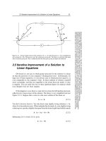
Fig. 5.3. Dynamically determined vertical modes for a continuously stratified
fluid: (a) stratification profile, N
2
(z); (b) vertical modes, G
m
(z) for m =
0, 1, 2.
When N
2
(z) > 0 at all heights, the eigenvalues from (5.48) and (5.50)
are countably infinite in number, positive in sign, and ordered by mag-
nitude: R
0
> R
1
> R
2
> . . . > 0. The eigenmodes satisfy the orthonor-
mality condition (5.32). Fig. 5.3 illustrates the shapes of the G
m
(z)

for the first few m with a stratification profile, N(z), that is upward-
intensified. For m = 0 (barotropic mode), G
0
(z) = 1, corresponding to
R
0
= ∞. For m ≥ 1 (baroclinic modes), G
m
(z) has precisely m zero-
crossings in z, so larger m corresponds to smaller vertical scales and
smaller deformation radii, R
m
. Note that the discrete modes in (5.35)
for N = 2 have the same structure as in Fig. 5.3, except for having a
finite truncation level, M = N −1. (The relation, H
1
> H
2
, in (5.35) is
analogous to an upward-intensified N(z) profile.)
5.2 Baroclinic Instability
The 2-layer quasigeostrophic model is now used to examine the stability
problem for a mean zonal current with vertical shear (Fig. 5.4). This is
the simplest flow configuration exhibiting baroclinic instability (cf., the
3D baroclinic instability in exercise #8 of this chapter). Even though
5.2 Baroclinic Instability 179
u
2
= − U
z

x
u
1
= + U
Fig. 5.4. Mean zonal baroclinic flow in a 2-layer fluid.
the Shallow-Water Equations (Chap. 4) contain some of the combined
effects of rotation and stratification, they do so incompletely compared
to fully 3D dynamics and, in particular, do not admit baroclinic insta-
bility because they cannot represent vertical shear.
In this analysis, for simplicity, assume that H
1
= H
2
= H/2; hence
the baroclinic deformation radius (5.39) is
R =

g

I
H
1
2f
.
This choice is a conventional idealization for the stratification in the
mid-latitude troposphere, whose mean stability profile, N(z), is approx-
imately constant in z above the planetary boundary layer (Chap. 6)
and below the tropopause. Further assume that there is no horizontal
shear (thereby precluding any barotropic instability) and no barotropic
180 Baroclinic and Jet Dynamics

component to the mean flow:
u
n
= (−1)
(n+1)
U
ˆ
x , (5.51)
with U a constant. Geostrophically and hydrostatically related mean
fields are
ψ
n
= (−1)
n+1
Uy
h
2
= −
f
0
g

(
ψ
1
− ψ
2
) +
H
2

=
2f
0
Uy
g

I
+
H
2
h
1
= H − h
2
q
QG,n
= βy + (−1)
n+1
Uy
R
2
. (5.52)
In this configuration there is more light fluid to the south (in the north-
ern hemisphere), since
h
2
−H
2
< 0 for y < 0, and more heavy fluid to the
north. Making an association between light density and warm tempera-

ture, then the south is also warmer and more buoyant (cf., (5.9)). This
is similar to the mid-latitude, northern-hemisphere atmosphere, with
stronger westerly winds aloft (Fig. 5.1) and warmer air to the south.
Note that (5.51)-(5.52) is a conservative stationary state; i.e., ∂
t
= 0
in (5.7) if F
n
= 0. The
q
QG,n
are functions only of y, as are the ψ
n
.
So they are functionals of each other. Therefore, J[ψ
n
, q
QG,n
] = 0,
and ∂
t
q
QG,n
= 0. The fluctuation dynamics are linearized around this
stationary state. Define
ψ
n
=
ψ
n

+ ψ

n
q
QG,n
=
q
QG,n
+ q

QG,n
, (5.53)
and insert these into (5.13)-(5.14), neglecting purely mean terms, per-
turbation nonlinear terms (assuming weak perturbations), and non-
conservative terms:
∂q

QG,n
∂t
+
u
n
∂q

QG,n
∂x
+ v

n
∂

q
QG,n
∂y
= 0 , (5.54)
or, evaluating the mean quantities explicitly,
∂q

QG,1
∂t
+ U
∂q

QG,1
∂x
+ v

1

β +
U
R
2

= 0
∂q

QG,2
∂t
− U
∂q


QG,2
∂x
+ v

2

β −
U
R
2

= 0 . (5.55)
5.2 Baroclinic Instability 181
5.2.1 Unstable Modes
One can expect there to be normal-mode solutions in the form of
ψ

n
= Real

Ψ
n
e
i(kx+y−ωt)

, (5.56)
with analogous expressions for the other dependent variables, because
the linear partial differential equations in (5.55) have constant coeffi-
cients. Inserting (5.56) into (5.55) and factoring out the exponential

function gives
(C − U )

K
2
Ψ
1
+
1
2R
2
(Ψ
1
− Ψ
2
)

+

β +
U
R
2

Ψ
1
= 0
(C + U )

K

2
Ψ
2
−
1
2R
2
(Ψ
1
− Ψ
2
)

+

β −
U
R
2

Ψ
2
= 0 (5.57)
for C = ω/k and K
2
= k
2
+ 
2
. Redefine the variables by transforming

the layer amplitudes into vertical modal amplitudes by (5.36):
˜
Ψ
0
≡
1
2
(Ψ
1
+ Ψ
2
)
˜
Ψ
1
≡
1
2
(Ψ
1
− Ψ
2
) . (5.58)
These are the barotropic and baroclinic vertical modes, respectively. The
linear combinations of layer coefficients are the vertical eigenfunctions
associated with R
0
= ∞ and R
1
= R from (5.39). Now take the sum

and difference of the equations in (5.57) and substitute (5.58) to obtain
the following modal amplitude equations:

CK
2
+ β

˜
Ψ
0
− UK
2
˜
Ψ
1
= 0

C(K
2
+ R
−2
) + β

˜
Ψ
1
− U(K
2
− R
−2

)
˜
Ψ
0
= 0 . (5.59)
For the special case with no mean flow, U = 0, the first equation in
(5.59) is satisfied for
˜
Ψ
0
= 0 only if
C = C
0
= −
β
K
2
. (5.60)
˜
Ψ
0
is the barotropic vertical modal amplitude, and this relation is iden-
tical to the dispersion relation for barotropic Rossby waves with an infi-
nite deformation radius (Sec. 3.1.2). The second equation in (5.59) with
˜
Ψ
1
= 0 implies that if
C = C
1

= −
β
K
2
+ R
−2
. (5.61)
˜
Ψ
1
is the baroclinic vertical modal amplitude, and the expression for C
182 Baroclinic and Jet Dynamics
is the same as the dispersion relation for baroclinic Rossby waves with
finite deformation radius, R (Sec. 4.7).
When U = 0, (5.59) has non-trivial modal amplitudes,
˜
Ψ
0
and
˜
Ψ
1
,
only if the determinant for their second-order system of linear algebraic
equations vanishes, viz.,
[CK
2
+ β] [C(K
2
+ R

−2
) + β] − U
2
K
2
[K
2
− R
−2
] = 0 . (5.62)
This is the general dispersion relation for this normal-mode problem.
To understand the implications of (5.62) with U = 0, first consider
the case of β = 0. Then the dispersion relation can be rewritten as
C
2
= U
2
K
2
− R
−2
K
2
+ R
−2
. (5.63)
For all KR < 1 (i.e., the long waves), C
2
< 0. This implies that C is
purely imaginary with an exponentially growing modal solution (i.e., an

instability) and a decaying one, proportional to
e
−ikCt
= e
k Imag[C]t
.
This behavior is a baroclinic instability for a mean flow with shear only
in the vertical direction.
For U, β = 0, the analogous condition for C having a nonzero imagi-
nary part is when the discriminant of the quadratic dispersion relation
(5.62) is negative, i.e., P < 0 for
P ≡ β
2
(2K
2
+ R
−2
)
2
− 4(β
2
K
2
− U
2
K
4
(K
2
− R

−2
)) (K
2
+ R
−2
)
= β
2
R
−4
+ 4U
2
K
4
(K
4
− R
−4
) . (5.64)
Note that β tends to stabilize the flow because it acts to make P more
positive and thus reduces the magnitude of Imag [C] when P is negative.
Also note that in both (5.63) and (5.64) the instability is equally strong
for either sign of U (i.e., eastward or westward vertical shear).
The smallest value for P(K) occurs when
0 =
∂P
∂K
4
= 4U
2

(K
4
− R
−4
) + 4U
2
K
4
, (5.65)
or
K =
1
2
1/4
R
. (5.66)
At this K value, the value for P is
P = β
2
R
−4
− U
2
R
−8
. (5.67)
5.2 Baroclinic Instability 183
Therefore, a necessary condition for instability is
U > βR
2

. (5.68)
From (5.52) this condition is equivalent to the mean potential vorticity
gradients, d
y
q
QG,n
, having opposite signs in the two layers,
d
q
QG,1
dy
·
d
q
QG,2
dy
< 0 .
The instability requirement for a sign change in the mean (potential)
vorticity gradient is similar to the Rayleigh criterion for barotropic vor-
tex instability (Sec. 3.3.1), and, not surprisingly, a Rayleigh criterion
may also be derived for quasigeostrophic baroclinic instability.
Further analysis of P(K) shows other conditions for instability:
• KR < 1 is necessary (and it is also sufficient when β = 0).
• U >
1
2
β(R
−4
− K
4

)
−1/2
→ ∞ as K → R
−1
from below.
• U >
1
2
βK
−2
→ ∞ as K → 0 from above.
These relations support the regime diagram in Fig. 5.5 for baroclinic
instability. For any U > βR
2
, there is a perturbation length scale for
the most unstable mode that is somewhat greater than the baroclinic
deformation radius. Short waves (K
−1
< R) are stable, and very long
waves (K
−1
→ ∞) are stable through the influence of β.
When P < 0, the solution to (5.62) is
C = −
β(2K
2
+ R
−2
)
2K

2
(K
2
+ R
−2
)
±
i
√
−P
2K
2
(K
2
+ R
−2
)
. (5.69)
Thus the zonal phase propagation for unstable modes (i.e., the real part
of C) is to the west. From (5.69),
−
β
K
2
< Real [C] < −
β
K
2
+ R
−2

. (5.70)
The unstable-mode phase speed lies in between the barotropic and baro-
clinic Rossby wave speeds in (5.60)-(5.61). This result is demonstrated
by substituting the first term in (5.69) for Real [C] and factoring −β/K
2
from all three expressions in (5.70). These steps yield
1 ≥
1 + µ/2
1 + µ
≥
1
1 + µ
(5.71)
for µ = (KR)
−2
. These inequalities are obviously true for all µ ≥ 0.
184 Baroclinic and Jet Dynamics
2
β
UK
2
=
βR
2
U
KR
2
−1/4
1
STABLE

UNSTABLE
U =
2
βR
2
(1−K
−1/2
)
4
R
4
Fig. 5.5. Regime diagram for baroclinic instability. The solid line indicates the
marginal stability curve as a function of the mean vertical shear amplitude,
U, and perturbation wavenumber, K, for β = 0. The vertical dashed line is
the marginal stability curve for β = 0.
5.2.2 Upshear Phase Tilt
From (5.59),
˜
Ψ
1
=
C + βK
−2
U
˜
Ψ
0
=




C + βK
−2
U



e
iθ
˜
Ψ
0
, (5.72)
where θ is the phase angle for (C + βK
−2
)/U in the complex plane.
Since
Real

C + βK
−2
U

> 0 (5.73)
from (5.70), and
Imag

C + βK
−2
U


=
Imag [C]
U
> 0 (5.74)
5.2 Baroclinic Instability 185
ψ’
~
ψ’
ψ’
~
ψ’
ψ’
~
0
1
2
+
−
’
~
ψ
0
1
1
+
+
= =
x
Fig. 5.6. Modal and layer phase relations for the perturbation streamfunction,

ψ

(x, t), in baroclinic instability for a 2-layer fluid. This plot exhibits graphical
addition: in each column the modal curves in the top two rows are added
together to obtain the respective layer curves in the bottom row.
for growing modes (with Real [−ikC] > 0, i.e., Imag [C] > 0), then
0 < θ < π/2 in westerly wind shear (U > 0). As shown in Fig. 5.6
this implies that
˜
ψ
1
has its pattern shifted to the west relative to
˜
ψ
0
,
by an amount less than a quarter wavelength. A graphical addition and
subtraction of
˜
ψ
1
and
˜
ψ
0
according to (5.58) is shown in Fig. 5.6. It
indicates that the layer ψ
1
has its pattern shifted to the west relative
to ψ

2
, by an amount less than a half wavelength. Therefore, upper-
layer disturbances are shifted to the west relative to lower-layer ones;
i.e., they are tilted upstream with respect to the mean shear direction
(Fig. 5.7). This feature is usually evident on weather maps during the
amplifying phase for mid-latitude cyclonic synoptic storms and is often
used as a synoptic analyst’s rule of thumb.
5.2.3 Eddy Heat Flux
Now calculate the poleward eddy heat flux,
v

T

(disregarding the con-
version factor, ρ
o
c
p
, between temperature and heat; Sec. 2.1.2). The
heat flux is analogous to a Reynolds stress (Sec. 3.4) as a contributor
to the dynamical balance relations for the equilibrium state, except it
186 Baroclinic and Jet Dynamics
ψ ’ (x,z)u(z)
x
z
+
+
+
+
+

−
+
−
− −
−
−
Fig. 5.7. Up-shear phase tilting for the perturbation streamfunction, ψ

(x, t),
in baroclinic instability for a continuously stratified fluid.
appears in the mean heat equation rather than the mean momentum
equation. Here v

= ∂
x
ψ

, and the temperature fluctuation is associated
with the interfacial displacement as in (5.9),
T

=
b

αg
=
1
αg
∂φ


∂z
=
f
αg
∂ψ

∂z
=
2f
αgH
(ψ

1
− ψ

2
) =
4f
αgH
˜
ψ

1
,
with all the proportionality constants positive in the northern hemi-
sphere. Suppose that at some time the modal fields have the (x, z)
structure,
˜
ψ


1
= A
1
sin[kx + θ]
˜
ψ

0
= A
0
sin[kx] (5.75)
for A
0
, A
1
> 0 and 0 < θ < π/2 (Fig. 5.6). Then
˜v

1
= A
1
k cos[kx + θ]
˜v

0
= A
0
k cos[kx] . (5.76)
The layer velocities, v


n
, are proportional to the sum of ˜v

0
and ±˜v

1
in the
upper and lower layers, respectively, as in (5.37). Therefore the modal
heat fluxes are
˜v

1
T

≡
k
2π

2π
0
dx ˜v

1
T

∝

2π
0

dx sin[kx + θ] cos[kx + θ] = 0
5.2 Baroclinic Instability 187
˜v

0
T

≡
k
2π

2π
0
dx ˜v

0
T

∝
k
2π

2π
0
dx sin[kx + θ] cos[kx] =
sin[θ]
2
(5.77)
with positive proportionality constants. Since each v


n
has a positive
contribution from ˜v

0
, the interfacial heat flux,
v

T

, is proportional to
˜v

0
T

, and it is therefore positive, v

T

> 0. The sign of v

T

is directly
related to the range of values for θ, i.e., to the upshear vertical phase
tilt (Sec. 5.2.2).
5.2.4 Effects on the Mean Flow
The nonzero eddy heat flux for baroclinic instability implies there is
an eddy–mean interaction. A mean energy balance is derived similarly

to the energy conservation relation (5.16) by manipulation of the mean
momentum and thickness equations. The result has the following form
in the present context:
d
dt
E = . . . +
 
dx dy g

I
v

η

d
η
dy
, (5.78)
where the dots refer to any non-conservative processes (here unspecified)
and the mean-flow energy is defined by
E =
 
dx dy
1
2

h
1
u
2

1
+ h
2
u
2
2
+ g

I
η
2

. (5.79)
Analogous to (3.100) for barotropic instability, there is a baroclinic en-
ergy conversion term here that generates fluctuation energy by removing
it from the mean energy when the eddy flux,
v

η

, has the opposite sign
to the mean gradient, d
y
η. Since η is proportional to T in a layered
model, this kind of conversion occurs when
v

T

> 0 and d

y
T < 0 (as
shown in Sec. 5.2.3).
The eddy–mean interaction cannot be fully analyzed in the spatially
homogeneous formulation of this section, implicit in the horizontally
periodic eigenmodes (5.56). It is the divergence of the eddy heat flux
that causes changes in the mean temperature gradient,
∂
T
∂t
= . . . −
∂
∂y
v

T

,
and the divergence is zero in a homogeneous flow. Thus, a more complete
interpretation of the role of eddies in the general circulation requires an
188 Baroclinic and Jet Dynamics
extension to inhomogeneous flows, such as the tropospheric westerly jet
that has its maximum speed at a middle latitude, ≈ 45
o
.
The poleward heat flux in baroclinic instability tends to weaken the
mean state by transporting warm air fluctuations into the region on the
poleward side of the jet with its associated mean-state cold air (n.b.,
Fig. 5.1). Equation (5.78) shows that the mean circulation loses energy
as the unstable fluctuations grow in amplitude: the mean meridional

temperature gradient (hence the mean geostrophic shear) is diminished
by the eddy heat flux, and part of the mean available potential en-
ergy associated with the meridional temperature gradient is converted
into eddy energy. The mid-latitude atmospheric climate is established
as a balance between the acceleration of the westerly Jet Stream by
Equator-to-pole differential radiative heating and the limitation of the
jet’s vertical shear strength by the unstable eddies that transport heat
between the Equatorial heating and polar cooling zones.
A similar interpretation can be made for the zonally directed Antarc-
tic Circumpolar Current (ACC) in the ocean (Fig. 6.11). In the wind-
driven ACC, the more natural dynamical characterization is in terms of
the mean momentum balance rather than the mean heat balance, al-
though these two balances must be closely related because of thermal
wind balance. A mean eastward wind stress beneath the westerly winds
drives a surface-intensified, eastward mean current that is baroclinically
unstable and generates eddies that transfer momentum vertically. This
eddy momentum transfer has to be balanced against a bottom turbulent
drag and/or topographic form stress (a pressure force against the solid
bottom topography; Sec. 5.3.3). The eddies also transport heat south-
ward (poleward in the Southern Hemisphere), balanced by the advective
heat flux caused by the mean, ageostrophic, secondary circulation in the
meridional (y, z) plane, such that there is no net heat flux by their com-
bined effects.
In these descriptions for the baroclinically unstable westerly winds
and ACC, notice two important ideas about the dynamical maintenance
of a mean zonal flow:
• An equivalence between horizontal heat flux and vertical momentum
flux for quasigeostrophic flows. The latter process is referred to as
isopycnal form stress. It is analogous to topographic form stress ex-
cept that the relevant material surface is an isopycnal in the fluid

interior instead of the solid bottom. Isopycnal form stress is not the
vertical Reynolds stress, < u

w

>, which is much weaker than the
5.3 Turbulent Baroclinic Zonal Jet 189
isopycnal form stress for quasigeostrophic flows because w

is so weak
(Sec. 4.7).
• The existence of a mean secondary circulation in the (y, z) plane,
perpendicular to the main zonal flow, associated with the eddy heat
and momentum fluxes whose mean meridional advection of heat may
partly balance the poleward eddy heat flux. This is called the Deacon
Cell for the ACC and the Ferrel Cell for the westerly winds. It also
is referred to as the meridional overturning circulation.
In the next section these behaviors are illustrated in an idealized prob-
lem for the statistical equilibrium state of an inhomogeneous zonal jet,
and the structures of the mean flow, eddy fluxes, and secondary circu-
lation are examined.
5.3 Turbulent Baroclinic Zonal Jet
5.3.1 Posing the Jet Problem
Consider a computational solution for a N-layer quasigeostrophic model
(Sec. 5.1.2) that demonstrates the phenomena discussed at the end of
the previous section. The problem could be formulated for a zonal jet
forced either by a meridional heating gradient (e.g., the mid-latitude
westerly winds in the atmosphere) or by a zonal surface stress (e.g.,
the ACC in the ocean). The latter is adopted because it embodies the
essentially adiabatic dynamics in baroclinic instability and its associated

eddy–mean interactions. It is an idealized model for the ACC, neglecting
both the actual wind and basin geographies and the diabatic surface
fluxes and interior mixing. For historical reasons (McWilliams & Chow,
1981), a solution is presented here with N set to 3; this is a N value
larger by one than the minimum vertical resolution, N = 2, needed to
represent baroclinic instability (Sec. 5.2).
This idealization for the ACC is as an adiabatic, quasigeostrophic,
zonally periodic jet driven by a broad, steady, zonal surface wind stress.
The flow environment is a Southern-hemisphere, β-plane approximation
to the Coriolis frequency and has an irregular bottom topography (which
can be included in the bottom layer of a N -layer model analogous to its
inclusion in a shallow-water model; Sec. 4.1). The mean stratification is
specified so that the baroclinic deformation radii, the R
m
from (5.46),
are much smaller than both the meridional wind scale, L
τ
, and the ACC
meridional velocity scale, L; the latter are also specified to be comparable
to the domain width, L
y
(i.e., R
m
 L, L
τ
, L
y
∀ m ≥ 1). This
190 Baroclinic and Jet Dynamics
s

(y)τ
x
1.5
η
1.5
η
η
N−.5
ρ
2
ρ
1
ρ
N
f =∇ βy
f/2 z
− g z
η
2.5
h
1
= H
1
−
h
2
= H
2
+ −
h

N
= H
N
+
z = H
z = B(x,y)
y
x
z
−B
Fig. 5.8. Posing the zonal jet problem for a N-layer model for a rotating,
stratified fluid on the β plane with surface wind stress and bottom topography.
The black dots indicate deleted intermediate layers for n = 3 to N −1.
problem configuration is sketched in Fig. 5.8. Another important scale is
L
β
=

V/β, with V a typical velocity associated with either the mean
or eddy currents. This is the Rhines scale (Sec. 4.8.1). In both the ACC
and this idealized solution, L
β
is somewhat smaller than L
y
, although
not by much. The domain is a meridionally bounded, zonally periodic
channel with solid side boundary conditions of no normal flow and zero
lateral stress. However, since the wind stress decays in amplitude away
from the channel center toward the walls, as do both the mean zonal jet
and its eddies, the meridional boundaries do not play a significant role

in the solution behavior (cf., the essential role of a western boundary
current in a wind gyre; Sec. 6.2). The resting layer depths are chosen
to have the values, H
n
= [500, 1250, 3250] m. They are unequal in
size, as is commonly done to represent the fact that mean stratification,
N(z), increases in the upper ocean. The reduced gravity values, g

n+.5
,
are then chosen so that the associated deformation radii are R
m
= [∞,
32, 15] km after solving the eigenvalue problem in Sec. 5.1.3, and these
values are similar to those for the real ACC. Both of the baroclinic R
m
(i.e., m ≥ 1) values are small compared to the chosen channel width of
L
y
= 1000 km.
5.3 Turbulent Baroclinic Zonal Jet 191
The wind stress accelerates a zonal flow. To have any chance of ar-
riving at an equilibrium state, the problem must be posed to include
non-conservative terms, e.g., with horizontal and vertical eddy viscosi-
ties (Sec. 3.5), ν
h
and ν
v
[m
2

s
−1
], and/or a bottom-drag damping co-
efficient, 
bot
[m s
−1
]. Non-conservative terms have not been discussed
very much so far, and they will merely be stated here in advance of the
more extensive discussion in Chap. 6. In combination with the imposed
zonal surface wind stress, τ
x
s
(y), these non-conservative quantities are
expressed in the non-conservative horizontal force as
F
1
=
τ
x
s
ρ
o
H
1
ˆ
x + ν
h
∇
2

u
1
+
2ν
v
H
1

u
2
− u
1
H
1
+ H
2

F
n
= ν
h
∇
2
u
n
+
2ν
v
H
n


u
n+1
− u
n
H
n
+ H
n+1
+
u
n−1
− u
n
H
n
+ H
n−1

,
2 ≤ n ≤ N − 1 ,
F
N
= ν
h
∇
2
u
N
+

2ν
v
H
N

u
N−1
− u
N
H
N
+ H
N−1

−

bot
H
N
u
N
. (5.80)
The wind stress is a forcing term in the upper layer (n = 1); the bottom
drag is a damping term in the bottom layer (n = N); the horizontal
eddy viscosity multiplies a second-order horizontal Laplacian operator
on u
n
, analogous to molecular viscosity (Sec. 2.1.2); and the verti-
cal eddy viscosity multiplies a finite-difference approximation to the
analogous second-order vertical derivative operating on u(z). In the

quasigeostrophic potential-vorticity equations (5.26)-(5.27), these non-
conservative terms enter as the force curl, F
n
. The potential-vorticity
equations are solved for the geostrophic layer streamfunctions, ψ
n
, and
the velocities in (5.80) are evaluated geostrophically.
The top and bottom boundary stress terms appear as equivalent body
forces in the layers adjacent to the boundaries. The underlying concept
for the boundary stress terms is that they are conveyed to the fluid in-
terior through turbulent boundary layers, called Ekman layers, whose
thickness is much smaller than the model’s layer thickness. So the verti-
cal flow structure within the Ekman layers cannot be explicitly resolved
in the layered model. Instead the Ekman layers are conceived of as thin
sub-layers embedded within the n = 1 and N resolved layers, and they
cause near-boundary vertical velocities, called Ekman pumping, at the
interior layer interfaces closest to the boundaries. In turn the Ekman
pumping causes vortex stretching in the rest of the resolved layer and
thereby acts to modify the layer’s thickness and potential vorticity. The
boundary stress terms in (5.80) have the net effects summarized here;
192 Baroclinic and Jet Dynamics
the detailed functioning of a turbulent boundary layer are explained in
Chap. 6.
If the eddy diffusion parameters are large enough (i.e., the effective
Reynolds number, Re, is small enough), they can viscously support a
steady, stable, laminar jet in equilibrium against the acceleration by the
wind stress. However, for smaller diffusivity values — as certainly re-
quired for geophysical plausibility — the accelerating jet will become un-
stable before it reaches a viscous stationary state. A bifurcation sequence

of successive instabilities with increasing Re values can be mapped out,
but most geophysical jets are well past this transition regime in Re. The
jets can reach an equilibrium state only through coexistence with a state
of fully developed turbulence comprised by the geostrophic, mesoscale ed-
dies generated by the mean jet instabilities. Accordingly, the values for
ν
h
and ν
v
in the computational solution are chosen to be small in or-
der to yield fully developed turbulence. The most important type of
jet instability for broad baroclinic jets, with L
y
 R
1
, is baroclinic in-
stability (Sec. 5.2). In fully developed turbulence the eddies grow by
instability of the mean currents, and they cascade the variance of the
fluctuations from their generation scale to the dissipation scale (cf., Sec.
3.7). In equilibrium the average rates for these processes must be equal.
In turn, the turbulent eddies limit and reshape the mean circulation (as
described at the end of Sec. 5.2.4) in an eddy–mean interaction.
5.3.2 Equilibrium Velocity and Buoyancy Structure
First consider the flow patterns and the geostrophically balanced buoy-
ancy field for fully developed turbulence in the statistical equilibrium
state that develops during a long-time integration of the 3-layer quasi-
geostrophic model. The instantaneous ψ
n
(x, y) and q
QG,n

(x, y) fields are
shown in Fig. 5.9, and the T (x, y) = b(x, y)/αg and w fields are shown
in Fig. 5.10 (n.b., f < 0 since this is for the southern hemisphere).
Note the strong, narrow, meandering jet in the upper ocean and the
weaker, broader flow in the abyssal ocean. The instantaneous centerline
for the jet is associated with a continuous front in b, a broken front in
q, and extrema in w alternating in sign within the eddies and along the
meandering jet axis.
The mean state is identified by an overbar defined as an average over
(x, t). The domain for each of these coordinates is taken to be infi-
nite, consistent with our interpretive assumptions of zonal homogeneity
and stationarity for the problem posed in Sec. 5.3.1, even though the
5.3 Turbulent Baroclinic Zonal Jet 193
ψ
1
ψ
3
x
y
x
xx
y
q
1
β y
q
3
yβ
− −
Fig. 5.9. Instantaneous horizontal patterns for streamfunction, ψ

n
, and quasi-
geostrophic potential vorticity, q
QG,n
(excluding its βy term), in the upper-
and lower-most layers in a zonal-jet solution with N = 3. The ψ contour
interval is 1.5 × 10
−4
m
2
s
−1
, and the q contour intervals are 2.5 (n = 1) and
0.25 (n = 3) ×10
−4
s
−1
. (McWilliams & Chow, 1981).
domain is necessarily finite (but large, for statistical accuracy) in a com-
putational solution. The combination of periodicity and translational
symmetry (literal or statistical) for the basin shape, wind stress, and to-
pography is a common finite-extent approximation to homogeneity. The
mean geostrophic flow is a surface intensified zonal jet,
u
n
(y), sketched
in Fig. 5.11. This jet is in hydrostatic, geostrophic balance with the
dynamic pressure,
φ
m

; streamfunction, ψ
n
; layer thickness, h
n
; interfa-
194 Baroclinic and Jet Dynamics
T
1.5
T
2.5
w
1.5
w
2.5
x
y
y
x
xx
Fig. 5.10. Instantaneous horizontal patterns for temperature, T
n+.5
, and ver-
tical velocity, w
n+.5
, at the upper and lower interior interfaces in a quasi-
geostrophic zonal-jet solution with N = 3. The T and w contour intervals are
0.4 and 0.1 K and 10
−4
m s
−1

and 0.5 ×10
−4
m s
−1
at the upper and lower
interfaces, respectively. (McWilliams & Chow, 1981).
cial elevation anomaly,
η
n+.5
; and interfacial buoyancy anomaly, b
n+.5
— each defined in Sec. 5.2 and sketched in Fig. 5.12.
The 3D mean circulation is (
u, v
a
, w). Only the zonal component is in
geostrophic balance. The meridional flow cannot be in geostrophic bal-
ance because there can be no mean zonal pressure gradient in a zonally
periodic channel, and vertical velocity is never geostrophic by defini-
tion (Sec. 2.4.2). Thus both components of the mean velocity in the
meridional plane (i.e., the meridional overturning circulation that is an
idealized form of the Deacon Cell; Sec. 5.2.4) is ageostrophic and thus
5.3 Turbulent Baroclinic Zonal Jet 195
u(y=0,z)
_
L /2
y
L /2
y
u

n
(y)
_
0
H
z
0
y
n=1n=2n=3
−
Fig. 5.11. Sketch of the time-mean zonal flow, u(y, z), in the equilibrium jet
problem with N = 3: (left) vertical profile in the middle of the channel and
(right) meridional profiles in different layers. Note the intensification of the
mean jet toward the surface and the middle of the channel.
u
N
y
u
1
u
2
z = H
z = B
y
z
x
north
n = 1
1.5
2

2.5
N−.5
N
h
N
h
2
h
1
warm
cool
ρ
1
ρ
2
ρ
N
n =
n =
n =
n =
n =
south
Fig. 5.12. Sketch of a meridional cross-section for the time-mean zonal jet,
the layer thickness, the density, and the buoyancy anomaly.
weaker than
u by O(Ro). The overturning circulation is sketched in Fig.
5.13. Because of the zonal periodicity, its component velocities satisfy a
2D continuity relation pointwise (cf., (4.112)):
∂

v
a
∂y
+
∂
w
∂z
= 0 . (5.81)
(A 2D zonally averaged continuity equation also occurs for the merid-
196 Baroclinic and Jet Dynamics
u
N
y
z
v v
v
v
w
w
u
1
u
2
z = H
z = B
north
n = 1
2
N
n =

n =
south
Fig. 5.13. Sketch of the time-mean, meridional overturning circulation (i.e.,
Deacon Cell) for the zonal jet, overlaid on the mean zonal jet and layer thick-
ness.
ional overturning circulation with solid boundaries in x, e.g., as in Sec.
6.2.) This relation will be further examined in the context of the layer
mass balance (Sec. 5.3.5).
The meridional profiles of mean and eddy-variance quantities in Figs.
5.14-5.15 show the following features:
• an eastward jet that increases its strength with height (cf., the atmo-
spheric westerly winds);
• geostrophically balancing temperature gradients (with cold water on
the poleward side of the jet);
• opposing potential vorticity gradients in the top and bottom layers
(i.e., satisfying a Rayleigh necessary condition for baroclinic instabil-
ity; Sec. 5.2.1);
• a nearly uniform q
QG,2
(y) in the middle layer (n.b., this is a conse-
quence of the eddy mixing of q
QG
, sometimes called potential-vorticity
homogenization, in a layer without significant non-conservative forces;
Sec. 5.3.4);
• mean upwelling on the poleward side of the jet and downwelling on the
Equatorward side (i.e., a Deacon Cell, the overturning secondary cir-
culation in the meridional plane, with an equatorward surface branch
that is Ekman-layer transport due to eastward wind stress in the
southern hemisphere; Chap. 6);

5.3 Turbulent Baroclinic Zonal Jet 197
yq∂
n
n
/ ∂
Hw
n+.5
n=1
2
3
1.5
2.5
1.5
2.5
n=1
n=1
2
2
3
3
n=1
2
2
n=1
3
3
ψ
n
u
n

(y) [m s
−1
]
H
n
q
T
n+.5
(y) [K]
6
6
6
m]y [10
m]
m]y [10
y [10
n
−1
](y) [m s
v
a,n
(y) [10 m s
−1
]
(y) [10 m ] s
−12
−1
]
[10 s ]
−1

(y) [10 m s
5
−3
−6 −7
0
1
2
0
1
2
0
1
2
0
10
−10
Fig. 5.14. Time-mean meridional profiles for a quasigeostrophic zonal-jet so-
lution with N = 3. The panels (clockwise from the upper right) are for
streamfunction, geostrophic zonal velocity, potential vorticity gradient, ver-
tical velocity, ageostrophic meridional velocity, temperature, and potential
vorticity. (McWilliams & Chow, 1981).
198 Baroclinic and Jet Dynamics
[x10]
n=1
n=1
n=1
2
2
2
3

3
1.5
2.5
3
]
2
(y) [m
2
v’
n
−2
s
T’ ]
2
’ψ
n+.5
2
(y) [K
[10y m]
6
[10y
6
m]
s(y) [m
2
u’
n
2
(y) [10 m ]
−2

s
44
]
−2
2
0
0
00
10
0.1
0.1
1
5
.5
.05
.05
n
Fig. 5.15. Meridional eddy variance profiles for a quasigeostrophic zonal-jet so-
lution with N = 3. The panels (clockwise from the upper right) are for stream-
function, geostrophic zonal velocity, temperature, and geostrophic meridional
velocity. (McWilliams & Chow, 1981).
• eddy variance profiles for ψ

, u

, v

, and T

= b


/αg that decay both
meridionally and vertically away from the jet core.
To understand how this equilibrium is dynamically maintained, the
mean dynamical balances for various quantities will be analyzed in Secs.
5.3.3-5.3.6. In each case the eddy flux makes an essential contribution
(cf., Sec. 3.4).