A Laboratory Course in C++Data Structures phần 8 doc
Bạn đang xem bản rút gọn của tài liệu. Xem và tải ngay bản đầy đủ của tài liệu tại đây (421.9 KB, 43 trang )
Weighted Graph ADT
|
285
Laboratory 13: Cover Sheet
Name __________________________________________ Date _______________________
Section _________________________________________
Place a check mark in the Assigned column next to the exercises your instructor has assigned to
you. Attach this cover sheet to the front of the packet of materials you submit following the
laboratory.
Activities
Prelab Exercise
Bridge Exercise
In-lab Exercise 1
In-lab Exercise 2
In-lab Exercise 3
Postlab Exercise 1
Postlab Exercise 2
Total
Assigned: Check or
list exercise numbers
Completed
Weighted Graph ADT
|
287
Laboratory 13: Prelab Exercise
Name __________________________________________ Date _______________________
Section _________________________________________
You can represent a graph in many ways. In this laboratory you will use an array to store the set
of vertices and an adjacency matrix to store the set of edges. An entry (j,k) in an adjacency matrix
contains information on the edge that goes from the vertex with index j to the vertex with index
k. For a weighted graph, each matrix entry contains the weight of the corresponding edge. A
specially chosen weight value is used to indicate edges that are missing from the graph.
The following graph yields the vertex list and adjacency matrix shown below. A ‘–’ is used to
denote an edge that is missing from the graph.
B
93
50
D
A
87
E
112
100
210
C
Vertex list
Adjacency matrix
Index
Label
From\To
0
1
2
3
4
0
A
0
—
50
100
—
—
1
B
1
50
—
—
93
—
2
C
2
100
—
—
112
210
3
D
3
—
93
112
—
87
4
E
4
—
—
210
87
—
Vertex A has an array index of 0 and vertex C has an array index of 2. The weight of the edge
from vertex A to vertex C is therefore stored in entry (0,2) in the adjacency matrix.
Step 1: Implement the operations in the Weighted Graph ADT using an array to store the vertices
(vertexList) and an adjacency matrix to store the edges (adjMatrix). The number of
vertices in a graph is not fixed; therefore, you need to store the maximum number of
vertices the graph can hold (maxSize) as well as the actual number of vertices in the
graph (size). Base your implementation on the following declarations from the file
wtgraph.h. An implementation of the showStructure operation is given in the file
show13.cpp.
288
|
Laboratory 13
const int defMaxGraphSize = 10,
vertexLabelLength = 11,
infiniteEdgeWt = INT_MAX;
// Default number of vertices
// Length of a vertex label
// “Weight” of a missing edge
class Vertex
{
public:
char label [vertexLabelLength];
// Vertex label
};
class WtGraph
{
public:
// Constructor
WtGraph ( int maxNumber = defMaxGraphSize )
throw ( bad_alloc );
// Destructor
~WtGraph ();
// Graph manipulation operations
void insertVertex ( Vertex newVertex )
throw ( logic_error );
void insertEdge ( char *v1, char *v2, int wt )
throw ( logic_error );
bool retrieveVertex ( char *v, Vertex &vData );
// Insert vertex
// Insert edge
//
bool getEdgeWeight ( char *v1, char *v2, int &wt )
throw ( logic_error );
//
void removeVertex ( char *v )
//
throw ( logic_error );
void removeEdge ( char *v1, char *v2 )
//
throw ( logic_error );
void clear ();
//
// Graph status operations
bool isEmpty () const;
bool isFull () const;
Get vertex
Get edge wt.
Remove vertex
Remove edge
Clear graph
// Graph is empty
// Graph is full
// Output the graph structure — used in testing/debugging
void showStructure ();
private:
// Facilitator functions
int getIndex ( char *v );
int getEdge ( int row, int col );
void setEdge ( int row, int col, int wt);
// Converts vertex label to
// an adjacency matrix
// index
//
//
//
//
Get edge weight using
Set edge weight using
adjacency matrix
indices
Weighted Graph ADT
// Data members
int maxSize,
size;
Vertex *vertexList;
int *adjMatrix;
//
//
//
//
Maximum number of vertices in the graph
Actual number of vertices in the graph
Vertex list
Adjacency matrix
};
Your implementations of the public member functions should use your getEdge() and
setEdge() facilitator functions to access entries in the adjacency matrix. For
example, the assignment statement
setEdge(2,3, 100);
uses the setEdge() function to assign a weight of 100 to the entry in the second row,
third column of the adjacency matrix. The if statement
if ( getEdge(j,k) == infiniteEdgeWt )
cout << “Edge is missing from graph” << endl;
uses this function to test whether there is an edge connecting the vertex with index j
and the vertex with index k.
Step 2: Save your implementation of the Weighted Graph ADT in the file
wtgraph.cpp. Be sure to document your code.
|
289
290
|
Laboratory 13
Laboratory 13: Bridge Exercise
Name __________________________________________ Date _______________________
Section _________________________________________
Check with your instructor whether you are to complete this exercise prior to your lab period
or during lab.
The test program in the file test13.cpp allows you to interactively test your implementation of
the Weighted Graph ADT using the following commands.
Command
+v
=v w wt
?v
#v w
-v
!v w
E
F
C
Q
Action
Insert vertex v.
Insert an edge connecting vertices v and w. The weight of this edge is wt.
Retrieve vertex v.
Retrieve the edge connecting vertices v and w and output its weight.
Remove vertex v.
Remove the edge connecting vertices v and w.
Report whether the graph is empty.
Report whether the graph is full.
Clear the graph.
Quit the test program.
Note that v and w denote vertex labels (type char*), not individual characters (type char). As a
result, you must be careful to enter these commands using the exact format shown above—
including spaces.
Step 1: Prepare a test plan for your implementation of the Weighted Graph ADT. Your test plan
should cover graphs in which the vertices are connected in a variety of ways. Be sure to
include test cases that attempt to retrieve edges that do not exist or that connect
nonexistent vertices. A test plan form follows.
Step 2: Execute your test plan. If you discover mistakes in your implementation, correct them
and execute your test plan again.
Weighted Graph ADT
Test Plan for the Operations in the Weighted Graph ADT
Test Case
Commands
Expected Result
Checked
|
291
|
292
Laboratory 13
Laboratory 13: In-lab Exercise 1
Name __________________________________________ Date _______________________
Section _________________________________________
In many applications of weighted graphs, you need to determine not only whether there is an edge
connecting a pair of vertices, but whether there is a path connecting the vertices. By extending the
concept of an adjacency matrix, you can produce a path matrix in which an entry (j,k) contains
the cost of the least costly (or shortest) path from the vertex with index j to the vertex with index
k. The following graph yields the path matrix shown below.
B
93
50
D
A
87
E
112
100
210
C
Vertex list
Path matrix
Index
Label
From/To:
0
1
2
3
4
0
A
0
0
50
100
143
230
1
B
1
50
0
150
93
180
2
C
2
100
150
0
112
199
3
D
3
143
93
112
0
87
4
E
4
230
180
199
87
0
This graph includes a number of paths from vertex A to vertex E. The cost of the least costly path
connecting these vertices is stored in entry (0,4) in the path matrix, where 0 is the index of vertex
A and 4 is the index of vertex E. The corresponding path is ABDE.
In creating this path matrix, we have assumed that a path with cost 0 exists from a vertex to
itself (entries of the form (j, j)). This assumption is based on the view that traveling from a vertex
to itself is a nonevent and thus costs nothing. Depending on how you intend to apply the
information in a graph, you may want to use an alternative assumption.
Given the adjacency matrix for a graph, we begin construction of the path matrix by noting
that all edges are paths. These one-edge-long paths are combined to form two-edge-long paths by
applying the following reasoning.
Weighted Graph ADT
If
then
there exists a path from a vertex j to a vertex m and
there exists a path from a vertex m to a vertex k,
there exists a path from vertex j to vertex k.
We can apply this same reasoning to these newly generated paths to form paths
consisting of more and more edges. The key to this process is to enumerate and
combine paths in a manner that is both complete and efficient. One approach to this
task is described in the following algorithm, known as Warshall’s algorithm. Note that
variables j, k, and m refer to vertex indices, not vertex labels.
Initialize the path matrix so that it is the same as the edge
matrix (all edges are paths). In addition, create a path with
cost 0 from each vertex back to itself.
for ( m = 0 ; m < size ; m++ )
for ( j = 0 ; j < size ; j++ )
for ( k = 0 ; k < size ; k++ )
If there exists a path from vertex j to vertex m and
there exists a path from vertex m to vertex k,
then add a path from vertex j to vertex k to the path matrix.
This algorithm establishes the existence of paths between vertices but not their
costs. Fortunately, by extending the reasoning used above, we can easily determine the
costs of the least costly paths between vertices.
If there exists a path from a vertex j to a vertex m and
there exists a path from a vertex m to a vertex k and
the cost of going from j to m to k is less than entry (j,k) in
the path matrix,
then replace entry (j,k) with the sum of entries (j,m) and (m,k).
Incorporating this reasoning into the previous algorithm yields the following
algorithm, known as Floyd’s algorithm.
Initialize the path matrix so that it is the same as the edge
matrix (all edges are paths). In addition, create a path with
cost 0 from each vertex back to itself.
for ( m = 0 ; m < size ; m++ )
for ( j = 0 ; j < size ; j++ )
for ( k = 0 ; k < size ; k++ )
If there exists a path from vertex j to vertex m and
there exists a path from vertex m to vertex k and
the sum of entries (j,m) and (m,k) is less than entry
(j,k) in the path matrix,
then replace entry (j,k) with the sum of entries (j,m)
and (m,k).
The following Weighted Graph ADT operation computes a graph’s path matrix.
|
293
294
|
Laboratory 13
void computePaths ()
Requirements:
None
Results:
Computes a graph’s path matrix.
Step 1: Add the data member
int *pathMatrix;
// Path matrix
and the function prototype
void computePaths ();
// Computes path matrix
to the WtGraph class declaration in the file wtgraph.h.
Step 2: Implement the computePaths operation described above and add it to the
file wtgraph.cpp.
Step 3: Replace the showStructure() function in the file wtgraph.cpp with a
showStructure() function that outputs a graph’s path matrix in addition to
its vertex list and adjacency matrix. An implementation of this function is
given in the file show14.cpp.
Step 4: Activate the “ PM ” (path matrix) test in the test program test13.cpp by
removing the comment delimiter (and the characters “PM”) from the lines that
begin with “//PM”.
Step 5: Prepare a test plan for the computePaths operation that includes graphs in
which the vertices are connected in a variety of ways with a variety of
weights. Be sure to include test cases in which an edge between a pair of
vertices has a higher cost than a multiedge path between these same vertices.
The edge CE and the path CDE in the graph shown earlier have this property.
A test plan form follows.
Step 6: Execute your test plan. If you discover mistakes in your implementation of
the computePaths operation, correct them and execute your test plan again.
Weighted Graph ADT
Test Plan for the computePaths Operation
Test Case
Commands
Expected Result
Checked
|
295
296
|
Laboratory 13
Laboratory 13: In-lab Exercise 2
Name __________________________________________ Date _______________________
Section _________________________________________
Suppose you wish to create a road map of a particular highway network. To avoid causing
confusion among map users, you must be careful to color the cities in such a way that no cities
sharing a common border also share the same color. An assignment of colors to cities that meets
this criterion is called a proper coloring of the map.
Restating this problem in terms of a graph, we say that an assignment of colors to the vertices
in a graph is a proper coloring of the graph if no vertex is assigned the same color as an adjacent
vertex. The assignment of colors (gray and white) shown in the following graph is an example of a
proper coloring.
B
F
C
Two colors are not always enough to produce a proper coloring. One of the most famous
theorems in graph theory, the Four-Color Theorem, states that creating a proper coloring of any
planar graph (that is, any graph that can be drawn on a sheet of paper without having the edges
cross one another) requires using at most four colors. A planar graph that requires four colors is
shown below. Note that if a graph is not planar, you may need to use more than four colors.
A
B
C
D
Weighted Graph ADT
The following Weighted Graph ADT operation determines whether a graph has a
proper coloring.
bool hasProperColoring () const
Requirements:
All the vertices have been assigned a color.
Results:
Returns true if no vertex in a graph has the same color as an adjacent vertex.
Otherwise, returns false.
Step 1: Add the following data member to the Vertex class declaration in the file
wtgraph.h.
char color;
// Vertex color (‘r’ for red and so forth)
Add the following function prototype to the WtGraph class declaration in the
file wtgraph.h.
bool hasProperColoring () const;
// Proper coloring?
Step 2: Implement the hasProperColoring operation described above and add it to
the file wtgraph.cpp.
Step 3: Replace the showStructure() function in the file wtgraph.cpp with a
showStructure() function that outputs a vertex’s color in addition to its
label. An implementation of this function is given in the file show13.cpp.
Step 4: Activate the “P” (proper coloring) command in the test program test13.cpp by
removing the comment delimiter (and the characters “PC”) from the lines that
begin with “//PC”.
Step 5: Prepare a test plan for the properColoring operation that includes a variety
of graphs and vertex colorings. A test plan form follows.
Step 6: Execute your test plan. If you discover mistakes in your implementation of
the properColoring operation, correct them and execute your test plan
again.
|
297
298
|
Laboratory 13
Test Plan for the properColoring Operation
Test Case
Commands
Expected Result
Checked
Weighted Graph ADT
|
299
Laboratory 13: In-lab Exercise 3
Name __________________________________________ Date _______________________
Section _________________________________________
A communications network consists of a set of switching centers (vertices) and a set of
communications lines (edges) that connect these centers. When designing a network, a
communications company needs to know whether the resulting network will continue to support
communications between all centers should one of these communications lines be rendered
inoperative due to weather or equipment failure. That is, they need to know the answer to the
following question.
Given a graph in which there is a path from every vertex to every other vertex, will removing any edge
from the graph always produce a graph in which there is still a path from every vertex to every other
vertex?
Obviously, the answer to this question depends on the graph. The answer for the graph shown
below is yes.
A
B
E
C
D
F
On the other hand, you can divide the following graph into two disconnected subgraphs by
removing the edge connecting vertices D and E. Thus, for this graph the answer is no.
A
B
E
G
C
D
F
H
Although determining an answer to this question for an arbitrary graph is somewhat difficult,
there are certain classes of graphs for which the answer is always yes. Given the definitions:
• A graph G is said to be connected if there exists a path from every vertex in G to every other
vertex in G.
• The degree of a vertex V in a graph G is the number of edges in G which connect to V, where
an edge from V to itself counts twice.
300
|
Laboratory 13
The following rule can be derived using simple graph theory:
If all of the vertices in a connected graph are of even degree, then removing any one edge
from the graph will always produce a connected graph.
If this rule applies to a graph, then you know that the answer to the previous question
is yes for that graph. Note that this rule tells you nothing about connected graphs in
which the degree of one or more vertices is odd.
The following Weighted Graph ADT operation checks whether every vertex in a
graph is of even degree.
bool areAllEven () const
Requirements:
None
Results:
Returns true if every vertex in a graph is of even degree. Otherwise, returns false.
Step 1: Implement the areAllEven operation described above and add it to the file
wtgraph.cpp. A prototype for this operation is included in the declaration of
the WtGraph class in the file wtgraph.h.
Step 2: Activate the ‘ D ’ (degree) command in the test program test13.cpp by
removing the comment delimiter (and the character ‘D’) from the lines that
begin with “//D”.
Step 3: Prepare a test plan for this operation that includes graphs in which the
vertices are connected in a variety of ways. A test plan form follows.
Step 4: Execute your test plan. If you discover mistakes in your implementation of
the areAllEven operation, correct them and execute your test plan again.
Weighted Graph ADT
Test Plan for the areAllEven Operation
Test Case
Commands
Expected Result
Checked
|
301
Weighted Graph ADT
|
303
Laboratory 13: Postlab Exercise 1
Name __________________________________________ Date _______________________
Section _________________________________________
Floyd’s algorithm (In-lab Exercise 1) computes the shortest path between each pair of vertices in a
graph. Suppose you need to know not only the cost of the shortest path between a pair of vertices,
but also which vertices lie along this path. At first, it may seem that you need to store a list of
vertices for every entry in the path matrix. Fortunately, you do not need to store this much
information. For each entry (j,k) in the path matrix, all you need to know is the index of the vertex
that follows j on the shortest path from j to k—that is, the index of the second vertex on the
shortest path from j to k. The following graph, for example,
B
93
50
D
A
87
E
112
100
210
C
yields the augmented path matrix shown below.
Vertex list
Path matrix (cost|second vertex on shortest path)
Index
Label
From/To
0
1
2
3
4
0
A
0
0|0
50|1
100|2
143|1
230|1
1
B
1
50|0
0|1
150|0
93|3
180|3
2
C
2
100|0
150|0
0|2
112|3
199|3
3
D
3
143|1
93|1
112|2
0|3
87|4
4
E
4
230|3
180|3
199|3
87|3
0|4
Entry (0,4) in this path matrix indicates that the cost of the shortest path from vertex A to vertex E
is 230. It further indicates that vertex B (the vertex with index 1) is the second vertex on the
shortest path. Thus the shortest path is of the form AB . . . E.
Explain how you can use this augmented path matrix to list the vertices that lie along the
shortest path between a given pair of vertices.
Weighted Graph ADT
|
305
Laboratory 13: Postlab Exercise 2
Name __________________________________________ Date _______________________
Section _________________________________________
Give an example of a graph for which no proper coloring can be created using less than five colors
(see In-lab Exercise 2). Does your example contradict the Four-Color Theorem?
Hash Table ADT
Implement the Hash Table ADT using an array of lists
representation
Use a hash table to implement a password-based
authentication system
Implement a perfect hash to store selected C++
reserved words
Implement a standard deviation analysis operation to
analyze the uniformity of the key distribution
Analyze the efficiency of your implementation of the
Hash Table ADT
Objectives
In this laboratory you will:
308
|
Laboratory 14
Overview
The data structures you have implemented up to this point are all useful and widely
used. However, their average performance for insertion and retrieval is generally O(N),
or at best O(log2N). As N becomes large—large is a relative term, depending on current
hardware configuration and performance, data record size and a number of other
factors, but let’s say hundreds of thousands or millions of records—O(N) becomes a
poor choice. Even O(log2N) performance can be unacceptable when handling many
simultaneous queries or processing large reports. How does searching, inserting, and
retrieving in O(1) sound? That is the possibility that the Hash Table ADT tries to offer.
Hash tables are among the fastest data structures for most operations and come closest
to offering O(1) performance. Consequently, a hash table is the preferred data structure
in many contexts. For instance, most electronic library catalogs are based on hash
tables.
The goal of the ideal hash table is to come up with a unique mapping of each key
onto a specific location in an array. The mapping of the key to a specific location in an
array is handled by the hash operation. A hash operation will accept the key as input
and return an integer that is used as an index into the hash table.
How does this work? The simplest case occurs when the key is an integer. Then the
hash function could simply return an integer. For instance, given the key 3, the hash
function would return the index value 3 to place the record in the hash table position
3. The key 1 would be used to place the record in hash table position 1.
Index
0
1
Key
2
3
1
4
5
6
3
But what about a key value of 8? The array used to implement the hash table does not
have a valid position 8, so some set of operations must be performed on the key in
order to map it to an index value that is valid for the array. A simple solution to this
problem is to perform a modulus operation with the table size on the key value. Using
the example of 8 for the table of size 7 above, the hash function would calculate 8
modulus 7 to produce an index value of 1.
Unfortunately, it is easy for the hash calculation to generate the same index value
for more than one key. This is called a collision. Using a key of 10 in the example
above, the hash calculation would produce 3—calculated as 10 modulus 7 (10%7 in
C++). But position 3 already has a key associated with it—the key 3. There are a
number of methods that can be used to resolve the collision. The one we use is called
chaining. When using chaining, all the keys that generate a particular index are
connected to that array position in a chain. One way to implement chaining is by
associating a list with each table entry. Using this approach, position 0 in the hash
table would have a list of all data items for which the hash operation produces an
index of 0, position 1 would have a list of all data items associated with index 1, and
so on through index 6. The key values 1, 3, 7, 8, 10, and 13 would produce the
following chains associated with the indexes 0, 1, 3, and 6.
Index
0
1
2
3
Key
7
1
3
8
10
4
5
6
13