Software Fault Tolerance Techniques and Implementation phần 5 pdf
Bạn đang xem bản rút gọn của tài liệu. Xem và tải ngay bản đầy đủ của tài liệu tại đây (1000.41 KB, 35 trang )
an executive that handles orchestrating and synchronizing the technique
(e.g., distributing the inputs, as shown), one or more additional variants
(versions) of the algorithm/program, and a DM. The versions are different
variants providing an incremental sort. For versions 1 and 2, a quick-
sort and bubble sort are used, respectively. Version 3 is the original incre-
mental sort.
Also note the design of the DM. It is straightforward to compare result
values if those values are individual numbers or strings (or other basic types).
How do we compare a list of values? Must all entries in all or a majority of
the lists be the same for success? Or can we compare each entry in the result
lists separately? Since the result of our sort is an ordered list, we can check
each entry against the entries in the same position in the other result lists. If
we designate the result in this example as r
ij
where i = 1, 2, 3 (up to n = 3 ver-
sions) and j = 1, 2, …, 6 (up to k = 6 items in the result set), then our DM
performs the following tests:
r
1j
= r
2j
= r
3j
where j = 1, …, k
If the r
ij
are equal for a specific j, then the result for that entry in the list is r
1j
(randomly selected since they are all equal). If they are not all equal for a spe-
cific j, do any two entries for a specific j match? That is, does
r
1j
= r
2j
OR r
1j
= r
3j
OR r
2j
= r
3j
where j = 1, …, k
If a match is found, the matching value is selected as the result for that posi-
tion in the list. If there is no match, that is, r
1j
≠ r
2j
≠ r
3j,
then there is no
correct result for that entry, designated by Ø.
Now, lets step through the example.
•
Upon entry to NVP, the executive performs the following: it for-
mats calls to the n = 3 versions and through those calls distributes
the inputs to the versions. The input set is (8, 7, 13, −4, 17, 44).
•
Each version, V
i
(i = 1, 2, 3), executes.
•
The results of the version executions (r
ij
, i = 1, , n; j = 1, , k) are
gathered by the executive and submitted to the DM.
126 Software Fault Tolerance Techniques and Implementation
TEAMFLY
Team-Fly
®
•
The DM examines the results as follows (shading indicates matching
results):
j r
1j
r
2j
r
3j
Result
−" −" −" −"
% % −% %
! & & −& &
" ! ! −! !
# % % −% %
$ "" "" −"" ""
•
The adjudicated result is (−4, 7, 8, 13, 17, 44).
•
Control returns to the executive.
• The executive passes the correct result, (−4, 7, 8, 13, 17, 44), outside
the NVP, and the NVP module is exited.
4.2.3 N-Version Programming Issues and Discussion
This section presents the advantages, disadvantages, and issues related to
NVP. As stated earlier in this chapter, software fault tolerance techniques
generally provide protection against errors in translating requirements and
functionality into code, but do not provide explicit protection against errors
in specifying requirements. This is true for all of the techniques described in
this book. Being a design diverse, forward recovery technique, NVP sub-
sumes design diversitys and forward recoverys advantages and disadvan-
tages, too. These are discussed in Sections 2.2 and 1.4.2, respectively. While
designing software fault tolerance into a system, many considerations have to
be taken into account. These are discussed in Chapter 3. Issues related to sev-
eral software fault tolerance techniques (such as similar errors, coincident
failures, overhead, cost, redundancy, etc.) and the programming practices
used to implement the techniques are described in Chapter 3. Issues related
to implementing voters are discussed in Section 7.1.
There are a few issues to note specifically for the NVP technique. NVP
runs in a multiprocessor environment, although it could be executed sequen-
tially in a uniprocessor environment. The overhead incurred (beyond that
of running a single version, as in non-fault-tolerant software) includes
additional memory for the second through the nth variants, executive,
and DM; additional execution time for the executive and the DM; and
Design Diverse Software Fault Tolerance Techniques %
synchronization overhead. The time overhead for the NVP technique is
always dependent upon the slowest variant, since all variant results must be
available for the voter to operate (for the basic majority voter). One solution
to the synchronization time overhead is to use a DM performing an algo-
rithm that operates on two or more results as they become available. (See
the self-configuring optimal programming (SCOP) technique discussion in
Section 6.4.)
In NVP operation, it is rarely necessary to interrupt the modules ser-
vice during voting. This continuity of service is attractive for applications
that require high availability.
To implement NVP, the developer can use the programming tech-
niques (such as assertions, atomic actions, idealized components) described
in Chapter 3. It is advised that the developer use the NVP paradigm
described in Section 3.3.3 to maximize the effectiveness of NVP by minimiz-
ing the chances of introducing related faults. There are three elements to the
NVP approach to software fault tolerance: the process of initial specification
and NVP, the product of that processthe N-version software (NVS)and
the environment that supports execution of NVS and provides decision algo-
rithmsthe N-version executive (NVX).
The purpose of the NVP design paradigm [60, 5] (see Section 3.3.3) is
to integrate NVP requirements and the software development methodol-
ogy. The objectives of the design paradigm are to (a) reduce the possibility of
oversights, mistakes, and inconsistencies in software development and testing;
(b) eliminate the most perceivable causes of remaining design faults; and (c)
minimize the probability that two or more variants produce similar erroneous
results during the same decision action. Not only must the design and develop-
ment be independent, but maintenance of the n variants must be performed
by separate maintenance entities or organizations to maintain independence.
It is critical that the initial specification for the variants used in NVP be
free of flaws. If the specification is flawed and the n programming teams use
that specification, then the variants are likely to produce indistinguishable
results. The success of NVP depends on the residual faults in each variant
being distinguishable, that is, that they cause disagreement in the decision
algorithm. Common mode failures or undetected similar errors among
a majority of the variants can cause an incorrect decision to be made by
the DM. Related faults among the variants and the DM also have to be mini-
mized. The similar error problem is the core issue in design diversity [61] and
has led to much research, some of it controversial (see [62]).
Also indistinguishable to voting-type decision algorithms are multiple
correct results (MCR) (see Section 3.1.1). Hence, NVP in general, and
128 Software Fault Tolerance Techniques and Implementation
voting-type decision algorithms in particular, are not appropriate for situa-
tions in which MCR may occur, such as in algorithms to find routes between
cities or finding the roots of an equation.
Using NVP to improve testing (e.g., in back-to-back testing) will likely
result in bugs being found that might otherwise not be found in single ver-
sion software [63]. However, testing the variants against one another with
comparison testing may cause the variants to compute progressively more
similar functions, thereby reducing the opportunity for NVP to tolerate
remaining faults [64].
Even though NVP utilizes the design diversity principle, it cannot be
guaranteed that the variants have no common residual design faults. If this
occurs, the purpose of NVP is defeated. The DM may also contain residual
design faults. If it does, then the DM may accept incorrect results or reject
correct results.
NVP does provide design diversity, but does not provide redundancy
or diversity in the data or data structures used. Independent design teams
may design data structures within each variant differently, but those struc-
tures global to NVP remain fixed [16]. This may limit the programmers
ability to diversify the variants.
Another issue in applying diverse, redundant software (this holds for
NVP and other design diverse software approaches) is determination of the
level at which the approach should be applied. The technique application
level influences the size of the resulting modules, and there are advantages
and disadvantages to both small and large modules. Stringini and Avizienis
[65] detail these as follows. Small modules imply:
•
Frequent invocations of the error detection mechanisms, resulting in
low error latency but high overhead;
•
Less computation must be redone in case of rollback, or less data
must be corrected by a vote (i.e., in NVP), but more temporary data
needs to be saved in checkpoints or voted upon;
•
The specifications common to the diverse implementations must be
similar to a higher level of detail. (Instead of specifying only what a
large module should do, and which variables must compose the state
of the computation outside that module, one needs to specify how
that large module is decomposed into smaller modules, what each
of the smaller modules does, and how it shall present its results to
the DM.)
Design Diverse Software Fault Tolerance Techniques '
Also needed for implementation and further examination of the tech-
nique is information on the underlying architecture and technique perfor-
mance. These are discussed in Sections 4.2.3.1 and 4.2.3.2, respectively.
Table 4.4 lists several NVP issues, indicates whether or not they are an
advantage or disadvantage (if applicable), and points to where in the book
the reader may find additional information.
The indication that an issue in Table 4.4 can be a positive or negative
(+/−) influence on the technique or on its effectiveness further indicates
130 Software Fault Tolerance Techniques and Implementation
Table 4.4
N-Version Programming Issue Summary
Issue
Advantage (+)/
Disadvantage (−) Where Discussed
Provides protec tion against errors in tr anslating
requirements an d functionality into code (true for
software fault to lerance techniques in ge neral)
+ Chapter 1
Does not provide explicit protection against errors
in specifying re quirements (true for soft ware fault
tolerance techn iques in general)
− Chapter 1
General forward recovery advantag es + Section 1.3.1.2
General forward recovery disadvan tages − Section 1.3.1.2
General design d iversity advantages + Section 2.2
General design d iversity disadvantages − Section 2.2
Similar errors o r common residual de sign errors − Section 3.1.1
Coincident and c orrelated failures − Section 3.1.1
MCR and identical and wrong results − Section 3.1.1
Consistent comparison problem (CCP) − Section 3.1.2
Overhead for tolerating a single fault +/− Section 3.1.4
Cost (Table 3.3) +/− Section 3.1.4
Space and time redundancy +/− Section 3.1.4
Design consider ations + Section 3.3.1
Dependable syst em development model + Section 3.3.2
NVS design paradigm + Section 3.3.3
Dependability s tudies +/− Section 4.1.3.3
Voters and discussions related to specific types
of voters
+/− Section 7.1
that the issue may be a disadvantage in general (e.g., cost is higher than non-
fault-tolerant software) but an advantage in relation to another technique.
In these cases, the reader is referred to the noted section for discussion of
the issue.
4.2.3.1 Architecture
We mentioned in Sections 1.3.1.2 and 2.5 that structuring is required if we
are to handle system complexity, especially when fault tolerance is involved
[1618]. This includes defining the organization of software modules onto
the hardware elements on which they run.
NVP is typically multiprocessor implemented with components resid-
ing on n hardware units and the executive residing on one of the processors.
Communications between the software components is done through remote
function calls or method invocations. Laprie and colleagues [19] provide
illustrations and discussion of architectures for NVP tolerating one fault and
that for tolerating two consecutive faults.
4.2.3.2 Performance
There have been numerous investigations into the performance of soft-
ware fault tolerance techniques in general (e.g., in the effectiveness of
software diversity, discussed in Chapters 2 and 3) and the dependability
of specific techniques themselves. Table 4.2 (in Section 4.1.3.3) provides
a list of references for these dependability investigations. This list, although
not exhaustive, provides a good sampling of the types of analyses that have
been performed and substantial background for analyzing software fault
tolerance dependability. The reader is encouraged to examine the references
for details on assumptions made by the researchers, experiment design, and
results interpretation. Laprie and colleagues [19] provide the derivation
and formulation of an equation for the probability of failure for NVP. A
comparative discussion of the techniques is provided in Section 4.7.
One way to improve the performance of NVP is to use a DM that
is appropriate for the problem solution domain. CV (see Section 7.1.4) is
one such alternative to majority voting. Consensus voting has the advantage
of being more stable than majority voting. The reliability of CV is at least
equivalent to majority voting. It performs better than majority voting when
average N-tuple reliability is low, or the average decision space in which vot-
ers work is not binary [53]. Also, when n is greater than 3, consensus voting
can make plurality decisions, that is, in situations where there is no majority
(the majority voter fails), the consensus voter selects as the correct result
the value of a unique maximum of identical outputs. A disadvantage of
Design Diverse Software Fault Tolerance Techniques 131
consensus voting is the added complexity of the decision algorithm. How-
ever, this may be overcome, at least in part, by pre-approved DM compo-
nents [66].
4.3 Distributed Recovery Blocks
The DRB technique (developed by Kane Kim [10, 67, 68]) is a combination
of distributed and/or parallel processing and recovery blocks that provides
both hardware and software fault tolerance. The DRB scheme has been
steadily expanded and supported by testbed demonstrations. Emphasis in the
development of the technique has been placed on real-time target applica-
tions, distributed and parallel computing systems, and handling both hard-
ware and software faults. Although DRB uses recovery blocks, it implements
a forward recovery scheme, consistent with its emphasis on real-time appli-
cations.
The techniques architecture consists of a pair of self-checking process-
ing nodes (PSP). The PSP scheme uses two copies of a self-checking comput-
ing component that are structured as a primary-shadow pair [69], resident on
two or more networked nodes. In the PSP scheme, each computing com-
ponent iterates through computation cycles and each of these cycles is two-
phase structured. A two-phase structured cycle consists of an input acquisi-
tion phase and an output phase. During the input acquisition phase, input
actions and computation actions may take place, but not output actions.
Similarly, during the output phase, only output actions may take place. This
facilitates parallel replicated execution of real-time tasks without incurring
excessive overhead related to synchronization of the two partner nodes in the
same primary-shadow structured computing station.
The structure and operation of the DRB are described in 4.3.1, with
an example provided in 4.3.2. Advantages, limitations, and issues related to
the DRB are presented in 4.3.3.
4.3.1 Distributed Recovery Block Operation
As shown in Figure 4.6, the basic DRB technique consists of a primary node
and a shadow node, each cooperating and each running an RcB scheme. An
input buffer at each node holds incoming data, released upon the next cycle.
The logic and time AT is an acceptance test and WDT combination that
checks its local processing. The time AT is a WDT that checks the other
node in the pair. The same primary try blocks, alternate try blocks, and ATs
132 Software Fault Tolerance Techniques and Implementation
Design Diverse Software Fault Tolerance Techniques 133
Input
buffer
B
F
F
S
Y
Initial shadow node
Data
ID
Input
buffer
A B
F
Time
AT
Local
DB
F
S
X
Initial primary node
A
Predecessor computing station
Time
AT
Local
DB
Successor computing station
Initial first try block
AT: Acceptance test
DB: Database
S: Success
F: Failure
Initial second try block
Logic and time
AT
Logic and time
AT
Figu re 4.6 Distribute d recovery block structure. (From: [6 7], © 19 89, IEEE. Reprinted with perm ission.)
are used on both nodes. The local DB (database) holds the current local
result. The DRB technique operation has the following much-simplified,
single cycle, general syntax.
run RB1 on Node 1 (Initial Primary),
RB2 on Node 2 (Initial Shadow)
ensure AT on Node 1 or Node 2
by Primary on Node 1 or Alternate on Node 2
else by Alternate on Node 1 or Primary on Node 2
else failure exception
The DRB single cycle syntax above states that the technique executes
the recovery blocks on both nodes concurrently, with one node (the initial
primary node) executing the primary algorithm first and the other (the initial
shadow node) executing the alternate. The technique first attempts to ensure
the AT (i.e., produce a result that passes the AT) with the primary algorithm
on node 1s results. If this result fails the AT, then the DRB tries the result
from the alternate algorithm on node 2. If neither passes the AT, then back-
ward recovery is used to execute the alternate on Node 1 and the primary on
Node 2. The results of these executions are checked to ensure the AT. If nei-
ther of these results passes the AT, then an error occurs. If any of the results are
successful, the result is passed on to the successor computing station.
Both fault-free and failure scenarios for the DRB are described below.
During this discussion of the DRB operation, keep in mind the following.
The governing rule of the DRB technique is that the primary node tries to
execute the primary alternate whenever possible and the shadow node tries to
execute the alternate try block whenever possible. In examining these scenar-
ios, the following abbreviations and notations are used:
AT Acceptance test;
Check-1 Check the AT result of the partner node with the WDT on;
Check-1* Check the progress of and/or AT status of the partner node;
Check-2 Check the delivery success of the partner node with the
WDT on;
Status-1 Inform other node of pickup of new input;
Status-2 Inform other node of AT result;
Status-3 Inform that output was delivered to successor computing
station successfully.
The Check and Status notations above were defined in [70].
134 Software Fault Tolerance Techniques and Implementation
4.3.1.1 Failure-Free Operation
Table 4.5 describes the operation of the DRB technique when no failure or
exception occurs.
4.3.1.2 Failure ScenarioPrimary Fails AT, Alternate Passes on Backup Node
Table 4.6 outlines the operation of the DRB technique when the primary
try block (on the primary node) fails its AT and the alternate try block (on
the backup node) is successful. Differences between this scenario and the
failure-free scenario are in gray type.
Design Diverse Software Fault Tolerance Techniques 135
Table 4.5
Distributed Recovery Block Without Failure or Exception
Primary Node Backup Node
Begin the comput ing cycle (Cycle). Begin the comput ing cycle (Cycle).
Receive input da ta from predecessor comp uting
station (Input).
Receive input da ta from predecessor comp uting
station (Input).
Start the recovery block (Ensure). Start the recovery block (Ensure).
Inform the back up node of pickup of new i nput
(Status-1 message).
Inform the prim ary node of pickup of new input
(Status-1 message).
Run the primary try block (Try). Run the alternate try block (Try).
Test the primary try blocks results (AT). The
results pass the AT.
Test the alterna te try blocks results (AT). The
results pass the AT.
Inform backup n ode of AT success
(Status-2 message).
Inform primary node of AT success
(Status-2 message).
Check if backup node is up and operating
correctly. Has it taken Status-2 actions
during a preset maximum number of data
processing cycl es? (Check-1* Message)
Yes, backup is OK.
Check AT result of primary node (Check-1
message). It pass ed and was placed in the
buffer.
Deliver result to successor computing station
(SEND) and update local database with result.
Check to make su re the primary successfully
delivered result (Check-2 message).
[Wait]
Tell backup node that result was de livered
(Status-3 message).
Primary was suc cessful in delivering res ult (No
Timeout).
End this processing cycle. End this processing cycle.
4.3.1.3 Failure ScenarioPrimary Node Stops Processing
This scenario is briefly described because it greatly resembles the previous
scenario with few exceptions. If the primary node stops processing entirely,
then no update message (
Status-2) can be sent to the backup. The backup
136 Software Fault Tolerance Techniques and Implementation
Table 4.6
Operation of Distributed Recovery Block When the Primary Fails and the Alternate Is Successful
Primary Node Backup Node
Begin the comput ing cycle (Cycle). Begin the comput ing cycle (Cycle).
Receive input da ta from predecessor comp uting
station (Input).
Receive input da ta from predecessor
computing stati on (Input).
Start the recovery block (Ensure). Start the recovery block (Ensure).
Inform the back up node of pickup of new i nput
(Status-1 message).
Inform the prim ary node of pickup of new
input (Status-1 message).
Run the primary try block (Try). Run the alternate try block (Try).
Test the primary try blocks results (
AT). The
results fail the AT.
Test the alterna te try blocks results (AT).
The results pass the AT.
Inform backup n ode of AT failure (Status-2
message).
Inform primary node of AT success
(Status-2 message).
Attempt to become the backup rollback and
retry using alternate try block (on primary node)
using same data on which primary try block failed
(to keep the sta te consistent or local dat abase
up-to-date). As sume the role of backup no de.
Check AT result of primary node
(Check-1 message). The p rimary node
failed. Assume the role of primary node.
Deliver result to successor computing
station (SEND) and update local database
with result.
Test the alterna te try blocks results (AT). The
results pass the AT.
Tell primary nod e that result was delivered
(Status-3 message).
Inform backup n ode of AT success (Status-2
message).
Check AT result of backup node (Check-1
message). It pass ed and was placed in the buffer.
Check to make su re the backup node succes sfully
delivered resul t (Check-2 message).
Backup was successful in delivering resu lt (No
Timeout).
End this processing cycle. End this processing cycle.
TEAMFLY
Team-Fly
®
node detects the crash with the expiration of a local timer associated with the
Check-1 message. The backup node operates as if the primary failed its AT
(as shown in the right-hand column in Table 4.6). If the backup node had
stopped instead, there would be no need to change processing in the primary
node, since it would simply retain the role of primary.
4.3.1.4 Failure ScenarioBoth Fail
Table 4.7 outlines the operation of the DRB technique when the primary
try block (on the primary node) fails its AT and the alternate try block (on
the backup node) also fails its AT. Differences between this scenario and the
failure-free scenario are in gray type.
In this scenario, the primary and back-up nodes did not switch roles.
When both fail their AT, there are two (or more) alternatives for resumption
of roles: (1) retain the original roles (primary as primary, backup as backup)
or (2) the first node to successfully pass its AT assumes the primary role.
Option one is less complex to implement, but option two can result in faster
recovery when the retry of the initial primary node takes significantly longer
than that of the initial backup.
4.3.2 Distributed Recovery Block Example
This section provides an example implementation of the DRB technique.
Recall the sort algorithm used in the RcB technique example (Section 4.1.2
and Figure 4.2). The implementation produces incorrect results if one or
more of the inputs is negative. In a DRB implementation of fault tolerance
for this example, upon each node resides a recovery block consisting of the
original sort algorithm implementation as primary and a different algorithm
implemented for the alternate try block. The AT is the sum of inputs
and outputs AT used in the RcB technique example, with a WDT. See
Section 4.1.2 for a description of the AT. Look at Figure 4.6 for the follow-
ing description of the DRB components for this example:
•
Initial primary node X:
•
Input buffer;
•
Primary A: Original sort algorithm implementation;
•
Alternate B: Alternate sort algorithm implementation;
•
Logic and time AT: Sum of inputs and outputs AT with WDT;
•
Local database;
•
Time AT;
Design Diverse Software Fault Tolerance Techniques 137
•
Initial shadow node Y:
•
Input buffer;
•
Primary A: Alternate sort algorithm implementation;
138 Software Fault Tolerance Techniques and Implementation
Table 4.7
Operation of Distributed Recovery Block When Both the Primary and Alternate Try Blocks Fail
Primary Node Backup Node
Begin the comput ing cycle (Cycle). Begin the comput ing cycle (Cycle).
Receive input da ta from predecessor comp uting
station (Input).
Receive input da ta from predecessor comp uting
station (Input).
Start the recovery block (Ensure). Start the recovery block (Ensure).
Inform the back up node of pickup of new i nput
(Status-1 message).
Inform the prim ary node of pickup of new input
(Status-1 message).
Run the primary try block (Try). Run the alternate try block (Try).
Test the primary try blocks results (AT). The
results fail the AT.
Test the alterna te try blocks results (AT). The
results fail the AT.
Inform backup n ode of AT failure (Status-2
message).
Inform primary node of AT failure (Status-2
message).
Rollback and retry using alternate try block (on
primary node) us ing same data on which
primary try block failed (to keep the st ate
consistent or local database up-to-date) .
Rollback and retry using primary try block (on
backup node) usi ng same data on which
alternate try block failed (to keep the state
consistent or local database up-to-date) .
Test the alterna te try blocks results (AT). The
results pass the AT.
Test the primary try blocks results (AT). The
results pass the AT.
Inform backup n ode of AT success
(Status-2 message).
Inform primary node of AT success
(Status-2 message).
Check if backup node is up and operating
correctly. Has it taken Status-2 actions during a
preset maximum number of data processing
cycles? (Check-1* Message) Yes, backup
is OK.
Check AT result of primary node (Check-1
message). It pass ed and was placed in the
buffer.
Deliver result to successor computing station
(SEND) and update local database with result.
Check to make su re the primary node
successfully de livered result (Check-2
message).
Tell backup node that result was de livered
(Status-3 message).
Primary was suc cessful in delivering res ult (No
Timeout).
End this processing cycle. End this processing cycle.
•
Alternate B: Original sort algorithm implementation;
•
Logic and time AT: Sum of inputs and outputs AT with WDT;
•
Local database;
•
Time AT.
Table 4.8 describes the events occurring on both nodes during the con-
current DRB execution.
4.3.3 Distributed Recovery Block Issues and Discussion
This section presents the advantages, disadvantages, and issues related to the
DRB technique. In general, software fault tolerance techniques provide pro-
tection against errors in translating requirements and functionality into code
but do not provide explicit protection against errors in specifying require-
ments. This is true for all of the techniques described in this book. Being a
design diverse, forward recovery technique, the DRB subsumes design diver-
sitys and forward recoverys advantages and disadvantages, too. These are
discussed in Sections 2.2 and 1.4.2, respectively. While designing soft-
ware fault tolerance into a system, many considerations have to be taken
into account. These are discussed in Chapter 3. Issues related to several soft-
ware fault tolerance techniques (such as similar errors, coincident failures,
overhead, cost, redundancy, etc.) and the programming practices used to
implement the techniques are described in Chapter 3. Issues related to imple-
menting ATs are discussed in Section 7.2.
There are a few issues to note specifically for the DRB technique. The
DRB runs in a multiprocessor environment. When the results of the initial
primary nodes primary try block pass the AT, the overhead incurred
(beyond that of running the primary alone, as in non-fault-tolerant soft-
ware) includes running the alternate on the shadow node, setting the check-
points for both nodes, and executing the ATs on both nodes. When recovery
is required, the time overhead is minimal because maximum concurrency is
exploited in DRB execution.
The DRBs relatively low run-time overhead makes it a candidate for
use in real-time systems. The DRB was originally developed for systems such
as command and control in which data from one pair of processors is out-
put to another pair of processors. The extended DRB implements changes to
the DRB for application to real-time process control [71, 72]. Extensions
and modifications to the original DRB scheme have also been developed
Design Diverse Software Fault Tolerance Techniques !'
for a repairable DRB [70] and for use in a load-sharing multiprocessing
scheme [67].
As with the RcB technique, an advantage of the DRB is that it is natu-
rally applicable to software modules, versus whole systems. It is natural to
140 Software Fault Tolerance Techniques and Implementation
Table 4.8
Concurrent Events in an Example Distributed Recovery Block Execution
Primary Node Backup Node
Begin the comput ing cycle. Begin the comput ing cycle.
Receive input da ta from predecessor comp uting
station. Input is (8, 7, 13, −4, 17, 44). Sum the
inputs for later use by AT. (Sum of inputs = 85.)
Receive input da ta from predecessor comp uting
station. Input is (8, 7, 13, −4, 17, 44). Sum the
inputs for later use by AT. (Sum of inputs = 85.)
Start the recovery block. Start the recovery block.
Inform the back up node of pickup of new i nput. Inform the prima ry node of pickup of new i nput.
Run the primary try block (original sort
algorithm). Result = (−4, −7, −8, −13, −17,
−44).
Run the alternate try block (backup sort
algorithm). Result = (−4, 7, 8, 13, 17, 44).
Test the primary try blocks results. Sum of
inputs was 85; sum of results = −93, not equal.
The results fail the AT.
Test the alterna te try blocks results. Sum of
inputs was 85; sum of results = 85, equal. The
results pass the AT.
Inform backup n ode of AT failure. Inform primary nod e of AT success.
Attempt to become the backuprollb ack and
retry using alternate algorithm (on pri mary
node) using same data on which ori ginal sort
algorithm faile d. Result = (−4, 7, 8, 13, 17, 44).
Check AT result of primary node. The primary
node failed. Ass ume the role of primary no de.
Test the alterna te try blocks (backup so rt
algorithm) results. Sum of inputs was 85; sum
of results = 85, equal. The results p ass the AT.
Deliver result to successor computing station
and update local database with result.
Inform backup n ode of AT success. Tell primar y node that result was delivered.
Check AT result of backup node. It passed and
was placed in th e buffer.
Check to make su re the backup node
successfully de livered result.
Backup was successful in delivering resu lt.
End this processing cycle. End this processing cycle.
apply the DRB to specific critical modules or processes in the system without
incurring the cost and complexity of supporting fault tolerance for an entire
system.
Also similar to the RcB technique, effective DRB operation requires
simple, highly effective ATs. A simple, effective AT can be difficult to
develop and depends heavily on the specification (see Section 7.2). Timing
tests are essential parts of the ATs for DRB use in real-time systems.
The DRB technique can provide real-time recovery from processing
node omission failures and can prevent the follow-on nodes from process-
ing faulty values to the extent determined by the ATs detection coverage.
The following DRB station node omission failures are tolerated: those caused
by (a) a fault in the internal hardware of a DRB station, (b) a design defect in
the operating system running on internal processing nodes of a DRB station,
or (c) a design defect in some application software modules used within a
DRB station [68].
Kim [68] lists the following major useful characteristics of the DRB
technique.
• Forward recovery can be accomplished in the same manner regard-
less of whether a node fails due to hardware faults or software faults.
• The recovery time is minimal since maximum concurrency is
exploited between the primary and the shadow nodes.
•
The increase in the processing turnaround time is minimal because
the primary node does not wait for any status message from the
shadow node.
•
The cost-effectiveness and the flexibility of the DRB technique is
high because:
•
A DRB computing station can operate with just two try blocks
and two processing nodes;
•
The two try blocks are not required to produce identical results
and the second try block need not be as sophisticated as the first
try block.
However, the DRB technique does impose some restrictions on the use of
RcB. To be used in DRB, a recovery block should be two-phase structured
(see the DRB operational description earlier in Section 4.3). This restriction
is necessary to prevent the establishment of interdependency, for recovery,
among the various DRB stations.
Design Diverse Software Fault Tolerance Techniques "
To implement the DRB technique, the developer can use the program-
ming techniques (such as assertions, checkpointing, atomic actions, idealized
components) described in Chapter 3. Implementation techniques for the
DRB are discussed by Kim in [68]. Also needed for implementation and fur-
ther examination of the technique is information on the underlying architec-
ture and performance. These are discussed in Sections 4.3.3.1 and 4.3.3.2,
respectively. Table 4.9 lists several DRB issues, indicates whether or not they
are an advantage or disadvantage (if applicable), and points to where in the
book the reader may find additional information.
The indication that an issue in Table 4.9 can be a positive or negative
(+/−) influence on the technique or on its effectiveness further indicates that
the issue may be a disadvantage in general but an advantage in relation to
142 Software Fault Tolerance Techniques and Implementation
Table 4.9
Distributed Recovery Block Issue Summary
Issue
Advantage (+)/
Disadvantage (−) Where Discussed
Provides protec tion against errors in tr anslating
requirements an d functionality into code (true for
software fault to lerance techniques in ge neral)
+ Chapter 1
Does not provide explicit protection against errors
in specifying re quirements (true for soft ware fault
tolerance techn iques in general)
− Chapter 1
General forward recovery advantag es + Section 1.4.2
General forward recovery disadvan tages − Section 1.4.2
General design d iversity advantages + Section 2.2
General design d iversity disadvantages − Section 2.2
Similar errors o r common residual de sign errors
(The DRB is affected to a lesser degree th an other
forward recovery techniques.)
− Section 3.1.1
Coincident and c orrelated failures − Section 3.1.1
Domino effect − Section 3.1.3
Overhead for tolerating a single fault +/− Section 3.1.4
Cost (Table 3.3) +/− Section 3.1.4
Space and time redundancy +/− Section 3.1.4
Dependability s tudies +/− Section 4.1.3.3
ATs and discussions related to specific types of ATs +/− Section 7.2
another technique. In these cases, the reader is referred to the discussion of
the issue (versus repeating the discussion here).
4.3.3.1 Architecture
We mentioned in Sections 1.3.1.2 and 2.5 that structuring is required if we
are to handle system complexity, especially when fault tolerance is involved
[1618]. This includes defining the organization of software modules onto
the hardware elements on which they run.
The DRB uses multiple processors with the recovery block components
and executive residing on distributed hardware units. Communications
between the software components is done through remote function calls or
method invocations. Laprie and colleagues [19] provide illustrations and dis-
cussion of distributed architectures for recovery blocks tolerating one fault
and those for tolerating two consecutive faults.
4.3.3.2 Performance
There have been numerous investigations into the performance of soft-
ware fault tolerance techniques in general (e.g., in the effectiveness of
software diversity, discussed in Chapters 2 and 3) and the dependability
of specific techniques themselves. Table 4.2 (in Section 4.1.3.3) provides
a list of references for these dependability investigations. This list, although
not exhaustive, provides a good sampling of the types of analyses that have
been performed and substantial background for analyzing software fault
tolerance dependability. The reader is encouraged to examine the references
for details on assumptions made by the researchers, experiment design, and
results interpretation. A comparative discussion of the techniques is provided
in Section 4.7. Laprie and colleagues [19] provide the derivation and formu-
lation of an equation for the probability of failure for the DRB technique.
One DRB experiment will be mentioned here, with others noted
in Table 4.2 and in the comparative analysis of the techniques provided in
Section 4.7. Kim and Welch [67] demonstrated the feasibility of the DRB
using a radar tracking application. The most important results of the demon-
stration include the following.
•
The increase in the average response time went from 1.8 to 2.6 mil-
liseconds (this is small in relation to the maximum response time of
40 milliseconds for the application).
•
The average processor utilization for the AT was 8%.
•
Backup processing was not a significant portion of the total workload.
Design Diverse Software Fault Tolerance Techniques 143
4.4 N Self-Checking Programming
NSCP is a design diverse technique developed by Laprie, et al. [73, 19].
The hardware fault tolerance architecture related to NSCP is active dynamic
redundancy. Self-checking programming is not a new concept, having been
introduced in 1975 [74]. A self-checking program uses program redundancy
to check its own behavior during execution. It results from either the applica-
tion of an AT to a variants results or from the application of a comparator to
the results of two variants. Self-checking software was used as the basis of the
Airbus A-300, A-310, and A-320 [75] flight control systems and the Swedish
railways interlocking system.
The NSCP hardware architecture consists of four components grouped
in two pairs in hot standby redundancy, in which each hardware compo-
nent supports one software variant. NSCP software includes two variants and
a comparison algorithm or one variant and an AT on each hardware pair.
When the NSCP executes, one of the self-checking components is the
active component. The other components are hot spares. When the
active component fails, one of the spares is switched to for delivery of
the service. When a spare fails, the active component continues to deliver
the service as it did before the spare failed. This is called result switching.
The N in NSCP is typically even, with the NSCP modules executed
in pairs. (N can be odd, for instance, in the case where one variant is used
in both pairs. In this case, if there are four hardware components, N = 3.)
Since the pairs are executed concurrently, there is an executive or consistency
mechanism that controls any required synchronization of inputs and out-
puts. The self-checking group results are compared or otherwise assessed for
correction. If there is no agreement, then the pair results are discarded. If
there is agreement, then the pair results are compared with the other pairs
results. NSCP failure occurs if both pairs disagree or the pairs agree but pro-
duce different results. NSCP is thus vulnerable to related faults between the
variants.
NSCP operation is described in 4.4.1, with an example provided in
4.4.2. The advantages and disadvantages of NSCP are presented in 4.4.3.
4.4.1 N Self-Checking Programming Operation
The NSCP technique consists of an executive, n variants, and comparison
algorithm(s). The executive orchestrates the NSCP technique operation,
which has the general syntax (for n = 4):
144 Software Fault Tolerance Techniques and Implementation
run Variants 1 and 2 on Hardware Pair 1,
Variants 3 and 4 on Hardware Pair 2
compare Results 1 and 2 compare Results 3 and 4
if not (match) if not (match)
set NoMatch1 set NoMatch2
else set Result Pair 1 else set Result Pair 2
if NoMatch1 and not NoMatch2, Result = Result Pair 2
else if NoMatch2 and not NoMatch1, Result = Result Pair 1
else if NoMatch1 and NoMatch2, raise exception
else if not NoMatch1 and not NoMatch2
then compare Result Pair 1 and 2
if not (match), raise exception
if (match), Result = Result Pair 1 or 2
return Result
The NSCP syntax above states that the technique executes the n vari-
ants concurrently, on n/2 hardware pairs. The results of the paired variants
are compared (e.g., variant 1 and 2 results are compared, variant 3 and 4
results are compared). If any pairs results do not match, a flag is set indicat-
ing pair failure. If a single pair failure has occurred, then the nonfailing pairs
results are returned as the NSCP result. If both pairs failed to match, then an
exception is raised. If pair results match (i.e., result 1 = result 2 and result 3 =
result 4) then the results of the pairs are compared. If they match (i.e., result
1 = result 2 = result 3 = result 4), then the result is set as one of the matching
values and returned as the NSCP result. If the result of the pair matches does
not match, then an exception is raised.
NSCP operation is illustrated in Figure 4.7. The NSCP block is
entered and the inputs are distributed to the variants. Each variant executes
on the inputs and the pairs results are gathered. Perhaps the above verbal
description of the NSCP result selection clouds the fairly simple concept.
Another way of illustrating the result selection process follows in Figure 4.8.
4.4.2 N Self-Checking Programming Example
This section provides an example implementation of the NSCP tech-
nique. Recall the sort algorithm used in the RcB example (Section 4.1.2 and
Figure 4.2). Our original sort implementation produces incorrect results if
one or more of the inputs are negative. Lets look at how the NSCP might be
used to protect our system against faults arising from this error.
Design Diverse Software Fault Tolerance Techniques "#
Figure 4.9 illustrates an NSCP implementation of fault tolerance for
this example. Note the additional components needed for NSCP imple-
mentation: an executive that handles orchestrating and synchronizing the
technique, n = 4 variants of incremental sort functionality, and comparators.
Variant 1 is the original incremental sort; variant 2 uses the quicksort algo-
rithm; variant 3 uses a bubble sort algorithm; and variant 4 uses heapsort.
The comparators simply test if the values of its inputs (the variant results) are
equal.
Now, lets step through the example.
•
Upon entry to the NSCP, the executive formats calls to the n = 4
variants and through those calls distributes the inputs to the vari-
ants. The input set is (8, 7, 13, −4, 17, 44).
•
Each variant, V
i
(i = 1, 2, 3, 4), executes.
146 Software Fault Tolerance Techniques and Implementation
NSCP entry
Output selected
NSCP exit
Failure exception
Variant 1
Module outputs Module outputs
Pair agreement Pair agreement
NSCP
Distribute
inputs
Variant 2
Variant 3
Variant 1
Variant 1 Variant 4
Gather results Gather results
Select result or
raise exception
Pair
fails
Pair
fails
Select result or
raise exception
Select result or
raise exception
Gather
results
Figu re 4.7 N self-checking programming structure and operation.
TEAMFLY
Team-Fly
®
_
The results of variants 1 and 2
executions are gathered and
submitted to the comparator.
_
The results of variants 3 and 4
executions are gathered and
submitted to the comparator.
_
The comparator examines the
results as follows:
R
1
= (−4, −7, −8, −13, −17, −44)
R
2
= (−4, 7, 8, 13, 17, 44)
R
1
≠ R
2
Pair failure. Set NoMatch1
(to use the other pairs results).
_
The comparator examines the
results as follows:
R
3
= (−4, 7, 8, 13, 17, 44)
R
4
= (−4, 7, 8, 13, 17, 44)
R
3
= R
4
Pair agreement.
Pair result = (−4, 7, 8, 13, 17, 44).
Design Diverse Software Fault Tolerance Techniques 147
Pair 1 Pair 2
Pair agreement Pair agreement
Result =
Success
Pair 1 Pair 2
Pair agreement Pair agreement
Result =
Result =
Failure, raise exception
Failure, raise exception
Result =
Success (partial failure,
then switch)
Pair 1 Pair 2 Pair 1 Pair 2
Pair fails
switch to standby
Pair agreement
Pair fails Pair fails
≠
≠
≠
(a) (b)
(d)
(c)
Figu re 4.8 N self-checking programming r esult selection process examples (a) success,
(b) f ailure, (c) partial failure, an d (d) failure.
•
The pair results, the NoMatch1 flag, and (−4, 7, 8, 13, 17, 44) are
gathered and submitted to another comparator.
•
The comparator examines the results as follows:
If (NoMatch1 AND NOT NoMatch2) use pair 2s results:
The adjudicated result is (−4, 7, 8, 13, 17, 44).
•
Control returns to the executive.
•
The executive passes the correct result, (−4, 7, 8, 13, 17, 44), outside
the NSCP, and the NSCP module is exited.
148 Software Fault Tolerance Techniques and Implementation
Distribute
inputs
Variant 1:
Original
incremental sort
Variant 2:
Quicksort
Variant 3:
Bubble sort
Variant 4:
Heapsort
( 4, 7, 8, 13, 17, 44)− − − − − − ( 4, 7, 8, 13, 17, 44)− ( 4, 7, 8, 13, 17, 44)−( 4, 7, 8, 13, 17, 44)−
Comparator:
( 4, 7, 8, 13, 17, 44)
( 4, 7, 8, 13, 17, 44)
Set Switch 1
− − − − − − ≠
−
Pair failure
Comparator:
( 4, 7, 8, 13, 17, 44)
( 4, 7, 8, 13, 17, 44)
− =
−
Pair agreement
(8, 13, 17, 44)7,4,−
Comparator:
Input (Switch 1, ( 4, 7, 8, 13, 17, 44))
Result ( 4, 7, 8, 13, 17, 44)
−
= −
Output: ( 4, 7, 8, 13, 17, 44)−
Figu re 4.9 Example of N self-checking programming implementation.
4.4.3 N Self-Checking Programming Issues and Discussion
This section presents the advantages, disadvantages, and issues related to
NSCP. As stated earlier in this chapter, software fault tolerance techniques
generally provide protection against errors in translating requirements and
functionality into code, but do not provide explicit protection against errors
in specifying requirements. This is true for all of the techniques described
in this book. Being a design diverse, forward recovery technique, NSCP
subsumes design diversitys and forward recoverys advantages and disadvan-
tages, too. These are discussed in Sections 2.2 and 1.4.2, respectively. While
designing software fault tolerance into a system, many considerations have to
be taken into account. These are discussed in Chapter 3. Issues related to sev-
eral software fault tolerance techniques (e.g., similar errors, coincident fail-
ures, overhead, cost, and redundancy) and the programming practices used
to implement the techniques are described in Chapter 3.
There are a few issues to note specifically for the NSCP technique.
NSCP runs in a multiprocessor environment. The overhead incurred
(beyond that of running a single non-fault-tolerant component) includes
additional memory for the second through the nth variants, executive,
and DM (comparators); additional execution time for the executive and the
DMs; and synchronization (input consistency) overhead.
The NSCP delays results only for comparison and result switching and
rarely requires interruption of the modules service during the comparisons
or result switching. This continuity of service is attractive for applications
that require high availability.
In NVP, the variants cooperate via the voting DM to deliver a correct
result. In NSCP though, each variant is responsible for delivering an accept-
able result.
To implement NSCP, the developer can use the programming techniques
(such as assertions, atomic actions, and idealized components) described in
Chapter 3. The developer may use relevant aspects of the NVP paradigm
described in Section 3.3.3 to minimize the chances of introducing related faults.
As in NVP and other design diverse techniques, it is critical that the
initial specification for the variants used in NSCP be free of flaws. Common
mode failures or undetected similar errors among the variants can cause an
incorrect decision to be made by the comparators. Related faults among the
variants and the comparators also have to be minimized.
Another issue in applying diverse, redundant software (i.e., this holds
for NSCP and other design diverse software fault tolerance approaches) is
determination of the level at which the approach should be applied. The
Design Diverse Software Fault Tolerance Techniques "'
technique application level influences the size of the resulting modules, and
there are advantages and disadvantages to both small and large modules (see
Section 4.2.3 for a discussion).
NSCP is made up of self-checking components executing the same
functionality. Combined with its error compensation capability, this gives
the NSCP the important benefit of clearly defined error containment areas.
The transformation from an erroneous to a potentially error-free state con-
sists of simply switching to the nonfailed hot spare pair.
Also needed for implementation and further examination of the tech-
nique is information on the underlying architecture and technique per-
formance. These are discussed in Sections 4.4.3.1 and 4.4.3.2, respectively.
Table 4.10 lists several NSCP issues, indicates whether or not they are an
advantage or disadvantage (if applicable), and points to where in the book
the reader may find additional information.
The indication that an issue in Table 4.10 can be a positive or negative
(+/−) influence on the technique or on its effectiveness further indicates that
the issue may be a disadvantage in general but an advantage in relation to
another technique. In these cases, the reader is referred to the noted section
for discussion of the issue.
4.4.3.1 Architecture
We mentioned in Sections 1.3.1.2 and 2.5 that structuring is required if we
are to handle system complexity, especially when fault tolerance is involved
[1618]. This includes defining the organization of software modules onto
the hardware elements on which they run.
As stated earlier, the NSCP hardware architecture consists of four
components grouped in two pairs in hot standby redundancy, in which each
hardware component supports one software variant. NSCP software includes
two variants and a comparison algorithm or one variant and an AT on each
hardware pair. The executive also resides on one of the hardware compo-
nents. If the production of four variants is cost-prohibitive, then three vari-
ants can be distributed across the two hardware pairs with a single variant
duplicated across the pairs. Communications between the software compo-
nents is done through remote function calls or method invocations. Laprie
and colleagues [19] provide illustrations and discussion of architectures for
NSCP tolerating one fault and that for tolerating two consecutive faults.
4.4.3.2 Performance
There have been numerous investigations into the performance of soft-
ware fault tolerance techniques in general (e.g., in the effectiveness of
150 Software Fault Tolerance Techniques and Implementation