The art of software testing second edition phần 5 ppt

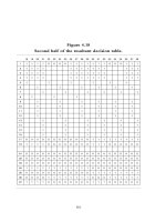
Figure 4.18
Second half of the resultant decision table.
18
1
19 20
1
21
1
22
0
23
0
24 25
0
26
10
27
1
28 29
1
30
1
31
1
32
11
33
0
3534
0
36

0
37
11
38
111
111 11111 1111121
111 11111 1111131
111 11111 1111141
1111151
1111116
1111117
1118
1111119
11111110
11111111
11111112
11111113
11111114
11111115
11111116
000000 0000011111111117 0
111000 0000011100000018 1
000000 0000000000000091 0
000000 0000000000000093 0
000000 0000000000000092 0
111111 1111100000000094 1
000000 0000011111111195 0
000111 1111100011111196 0
111000 0000011100000097 1
84

01.qxd 4/29/04 4:33 PM Page 84
20 DISPLAY 21-29 (94, 97)
21 DISPLAY 4021.A (94, 97)
22 DISPLAY –END (94, 96)
23 DISPLAY (94, 96)
24 DISPLAY –F (94, 96)
25 DISPLAY .E (94, 96)
26 DISPLAY 7FF8-END (94, 96)
27 DISPLAY 6000 (94, 96)
28 DISPLAY A0-A4 (94, 96)
29 DISPLAY 20.8 (94, 96)
30 DISPLAY 7001-END (95, 97)
31 DISPLAY 5-15 (95, 97)
32w DISPLAY 4FF.100 (95, 97)
33 DISPLAY –END (95, 96)
34 DISPLAY –20 (95, 96)
35 DISPLAY .11 (95, 96)
36 DISPLAY 7000-END (95, 96)
37 DISPLAY 4-14 (95, 96)
38 DISPLAY 500.11 (95, 96)
Note that where two or more different test cases invoked, for the
most part, the same set of causes, different values for the causes were
selected to slightly improve the yield of the test cases. Also note that,
because of the actual storage size, test case 22 is impossible (it will
yield effect 95 instead of 94, as noted in test case 33). Hence, 37 test
cases have been identified.
Remarks
Cause-effect graphing is a systematic method of generating test cases
representing combinations of conditions. The alternative would be
an ad hoc selection of combinations, but, in doing so, it is likely that

you would overlook many of the “interesting” test cases identified by
the cause-effect graph.
Since cause-effect graphing requires the translation of a specifica-
tion into a Boolean logic network, it gives you a different perspective
Test-Case Design 85
01.qxd 4/29/04 4:33 PM Page 85
on, and additional insight into, the specification. In fact, the devel-
opment of a cause-effect graph is a good way to uncover ambiguities
and incompleteness in specifications. For instance, the astute reader
may have noticed that this process has uncovered a problem in the
specification of the
DISPLAY command. The specification states that
all output lines contain four words. This cannot be true in all cases; it
cannot occur for test cases 18 and 26 since the starting address is less
than 16 bytes away from the end of memory.
Although cause-effect graphing does produce a set of useful test
cases, it normally does not produce all of the useful test cases that
might be identified. For instance, in the example we said nothing
about verifying that the displayed memory values are identical to the
values in memory and determining whether the program can display
every possible value in a memory location. Also, the cause-effect
graph does not adequately explore boundary conditions. Of course,
you could attempt to cover boundary conditions during the process.
For instance, instead of identifying the single cause
hexloc2 м hexloc1
you could identify two causes:
hexloc2 = hexloc1
hexloc2 > hexloc1
The problem in doing this, however, is that it complicates the graph
tremendously and leads to an excessively large number of test cases.

For this reason it is best to consider a separate boundary-value analy-
sis. For instance, the following boundary conditions can be identified
for the
DISPLAY specification:
1. hexloc1 has one digit.
2. hexloc1 has six digits.
3. hexloc1 has seven digits.
4. hexloc1 = 0.
86 The Art of Software Testing
01.qxd 4/29/04 4:33 PM Page 86
5. hexloc1 = 7FFF.
6. hexloc1 = 8000.
7. hexloc2 has one digit.
8. hexloc2 has six digits.
9. hexloc2 has seven digits.
10. hexloc2 = 0.
11. hexloc2 = 7FFF.
12. hexloc2 = 8000.
13. hexloc2 = hexloc1.
14. hexloc2 = hexloc1 + 1.
15. hexloc2 = hexloc1 − 1.
16. bytecount has one digit.
17. bytecount has six digits.
18. bytecount has seven digits.
19. bytecount = 1.
20. hexloc1 + bytecount = 8000.
21. hexloc1 + bytecount = 8001.
22. display 16 bytes (one line).
23. display 17 bytes (two lines).
Note that this does not imply that you would write 60 (37 + 23)

test cases. Since the cause-effect graph gives us leeway in selecting
specific values for operands, the boundary conditions could be
blended into the test cases derived from the cause-effect graph. In
this example, by rewriting some of the original 37 test cases, all 23
boundary conditions could be covered without any additional test
cases. Thus, we arrive at a small but potent set of test cases that satisfy
both objectives.
Note that cause-effect graphing is consistent with several of the
testing principles in Chapter 2. Identifying the expected output of
each test case is an inherent part of the technique (each column in
the decision table indicates the expected effects). Also note that it
encourages us to look for unwanted side effects. For instance, column
(test) 1 specifies that you should expect effect 91 to be present and
that effects 92 through 97 should be absent.
Test-Case Design 87
01.qxd 4/29/04 4:33 PM Page 87
The most difficult aspect of the technique is the conversion of the
graph into the decision table. This process is algorithmic, implying
that you could automate it by writing a program; several commercial
programs exist to help with the conversion.
Error Guessing
It has often been noted that some people seem to be naturally adept
at program testing. Without using any particular methodology such
as boundary-value analysis of cause-effect graphing, these people
seem to have a knack for sniffing out errors.
One explanation of this is that these people are practicing, sub-
consciously more often than not, a test-case-design technique that
could be termed error guessing. Given a particular program, they sur-
mise, both by intuition and experience, certain probable types of
errors and then write test cases to expose those errors.

It is difficult to give a procedure for the error-guessing technique
since it is largely an intuitive and ad hoc process. The basic idea is to
enumerate a list of possible errors or error-prone situations and then
write test cases based on the list. For instance, the presence of the
value 0 in a program’s input is an error-prone situation. Therefore,
you might write test cases for which particular input values have a 0
value and for which particular output values are forced to 0. Also,
where a variable number of inputs or outputs can be present (e.g., the
number of entries in a list to be searched), the cases of “none” and
“one” (e.g., empty list, list containing just one entry) are error-prone
situations. Another idea is to identify test cases associated with
assumptions that the programmer might have made when reading the
specification (i.e., things that were omitted from the specification,
either by accident or because the writer felt them to be obvious).
Since a procedure cannot be given, the next-best alternative is to
discuss the spirit of error guessing, and the best way to do this is by
presenting examples. If you are testing a sorting subroutine, the fol-
lowing are situations to explore:
88 The Art of Software Testing
01.qxd 4/29/04 4:33 PM Page 88
• The input list is empty.
• The input list contains one entry.
• All entries in the input list have the same value.
• The input list is already sorted.
In other words, you enumerate those special cases that may have been
overlooked when the program was designed. If you are testing a
binary-search subroutine, you might try the situations where (1)
there is only one entry in the table being searched, (2) the table size
is a power of two (e.g., 16), and (3) the table size is one less than and
one greater than a power of two (e.g., 15 or 17).

Consider the MTEST program in the section on boundary-value
analysis. The following additional tests come to mind when using the
error-guessing technique:
• Does the program accept “blank” as an answer?
• A type-2 (answer) record appears in the set of type-3 (student)
records.
• A record without a 2 or 3 in the last column appears as other
than the initial (title) record.
• Two students have the same name or number.
• Since a median is computed differently depending on whether
there is an odd or an even number of items, test the program
for an even number of students and an odd number of students.
• The number-of-questions field has a negative value.
Error-guessing tests that come to mind for the
DISPLAY command
of the previous section are as follows:
• DISPLAY 100- (partial second operand)
•
DISPLAY 100. (partial second operand)
•
DISPLAY 100-10A 42 (extra operand)
•
DISPLAY 000-0000FF (leading zeros)
Test-Case Design 89
01.qxd 4/29/04 4:33 PM Page 89
The Strategy
The test-case-design methodologies discussed in this chapter can be
combined into an overall strategy. The reason for combining them
should be obvious by now: Each contributes a particular set of useful
test cases, but none of them by itself contributes a thorough set of test

cases. A reasonable strategy is as follows:
1. If the specification contains combinations of input condi-
tions, start with cause-effect graphing.
2. In any event, use boundary-value analysis. Remember that
this is an analysis of input and output boundaries. The
boundary-value analysis yields a set of supplemental test con-
ditions, but, as noted in the section on cause-effect graphing,
many or all of these can be incorporated into the cause-effect
tests.
3. Identify the valid and invalid equivalence classes for the input
and output, and supplement the test cases identified above if
necessary.
4. Use the error-guessing technique to add additional test cases.
5. Examine the program’s logic with regard to the set of test
cases. Use the decision-coverage, condition-coverage, deci-
sion/condition-coverage, or multiple-condition-coverage
criterion (the last being the most complete). If the coverage
criterion has not been met by the test cases identified in the
prior four steps, and if meeting the criterion is not impossi-
ble (i.e., certain combinations of conditions may be impossi-
ble to create because of the nature of the program), add
sufficient test cases to cause the criterion to be satisfied.
Again, the use of this strategy will not guarantee that all errors will
be found, but it has been found to represent a reasonable compro-
mise. Also, it represents a considerable amount of hard work, but no
one has ever claimed that program testing is easy.
90 The Art of Software Testing
01.qxd 4/29/04 4:33 PM Page 90
CHAPTER 5
Module (Unit) Testing

Up to this point we have largely
ignored the mechanics of testing and the size of the program being
tested. However, large programs (say, programs of 500 statements or
more) require special testing treatment. In this chapter we consider
an initial step in structuring the testing of a large program: module
testing. Chapter 6 discusses the remaining steps.
Module testing (or unit testing) is a process of testing the individ-
ual subprograms, subroutines, or procedures in a program. That is,
rather than initially testing the program as a whole, testing is first
focused on the smaller building blocks of the program. The moti-
vations for doing this are threefold. First, module testing is a way
of managing the combined elements of testing, since attention is
focused initially on smaller units of the program. Second, module
testing eases the task of debugging (the process of pinpointing and
correcting a discovered error), since, when an error is found, it is
known to exist in a particular module. Finally, module testing intro-
duces parallelism into the program testing process by presenting us
with the opportunity to test multiple modules simultaneously.
The purpose of module testing is to compare the function of a
module to some functional or interface specification defining the
module. To reemphasize the goal of all testing processes, the goal
here is not to show that the module meets its specification, but to
show that the module contradicts the specification. In this chapter we
discuss module testing from three points of view:
1. The manner in which test cases are designed.
2. The order in which modules should be tested and integrated.
3. Advice about performing the test.
91
02.qxd 4/29/04 4:36 PM Page 91
Test-Case Design

You need two types of information when designing test cases for a
module test: a specification for the module and the module’s source
code. The specification typically defines the module’s input and out-
put parameters and its function.
Module testing is largely white-box oriented. One reason is that as
you test larger entities such as entire programs (which will be the case
for subsequent testing processes), white-box testing becomes less fea-
sible. A second reason is that the subsequent testing processes are ori-
ented toward finding different types of errors (for example, errors not
necessarily associated with the program’s logic, such as the program’s
failing to meet its users’ requirements). Hence, the test-case-design
procedure for a module test is the following: Analyze the module’s
logic using one or more of the white-box methods, and then supple-
ment these test cases by applying black-box methods to the module’s
specification.
Since the test-case-design methods to be used have already been
defined in Chapter 4, their use in a module test is illustrated here
through an example. Assume that we wish to test a module named
BONUS, and its function is to add $2,000 to the salary of all employ-
ees in the department or departments having the largest sales amount.
However, if an eligible employee’s current salary is $150,000 or
more, or if the employee is a manager, the salary is increased by only
$1,000.
The inputs to the module are the tables shown in Figure 5.1. If the
module performs its function correctly, it returns an error code of 0.
If either the employee or the department table contains no entries, it
returns an error code of 1. If it finds no employees in an eligible
department, it returns an error code of 2.
The module’s source code is shown in Figure 5.2. Input parame-
ters

ESIZE and DSIZE contain the number of entries in the employee
and department tables. The module is written in PL/1, but the fol-
lowing discussion is largely language independent; the techniques are
applicable to programs coded in other languages. Also, since the
92 The Art of Software Testing
02.qxd 4/29/04 4:36 PM Page 92
PL/1 logic in the module is fairly simple, virtually any reader, even
those not familiar with PL/1, should be able to understand it.
Regardless of which of the logic-coverage techniques you use, the
first step is to list the conditional decisions in the program. Candi-
dates in this program are all
IF and DO statements. By inspecting the
program, we can see that all of the
DO statements are simple iterations,
each iteration limit will be equal to or greater than the initial value
(meaning that each loop body always will execute at least once), and
the only way of exiting each loop is via the
DO statement. Thus, the
DO statements in this program need no special attention, since any test
case that causes a
DO statement to execute will eventually cause it to
Module (Unit) Testing 93
Figure 5.1
Input tables to module BONUS.
Dept. Salary
Job
code
Name Dept.
Department table
Employee table

Sales
02.qxd 4/29/04 4:36 PM Page 93
Figure 5.2
Module BONUS.
BONUS : PROCEDURE(EMPTAB,DEPTTAB,ESIZE,DSIZE,ERRCODE);
DECLARE 1 EMPTAB (*),
2 NAME CHAR(6),
2 CODE CHAR(1),
2 DEPT CHAR(3),
2 SALARY FIXED DECIMAL(7,2);
DECLARE 1 DEPTTAB (*),
2 DEPT CHAR(3),
2 SALES FIXED DECIMAL(8,2);
DECLARE (ESIZE,DSIZE) FIXED BINARY;
DECLARE ERRCODE FIXED DECIMAL(1);
DECLARE MAXSALES FIXED DECIMAL(8,2) INIT(0); /*MAX. SALES IN DEPTTAB*/
DECLARE (I,J,K) FIXED BINARY; /*COUNTERS*/
DECLARE FOUND BIT(1); /*TRUE IF ELIGIBLE DEPT. HAS EMPLOYEES*/
DECLARE SINC FIXED DECIMAL(7,2) INIT(200.00); /*STANDARD INCREMENT*/
DECLARE LINC FIXED DECIMAL(7,2) INIT(100.00); /*LOWER INCREMENT*/
DECLARE LSALARY FIXED DECIMAL(7,2) INIT(15000.00); /*SALARY BOUNDARY*/
DECLARE MGR CHAR(1) INIT('M');
1 ERRCODE=0;
2 IF(ESIZE<=0)|(DSIZE<=0)
3 THEN ERRCODE=1; /*EMPTAB OR DEPTTAB ARE EMPTY*/
4 ELSE DO;
5 DO I = 1 TO DSIZE; /*FIND MAXSALES AND MAXDEPTS*/
6 IF(SALES(I)>=MAXSALES) THEN MAXSALES=SALES(I);
7 END;
8 DO J = 1 TO DSIZE;

9 IF(SALES(J)=MAXSALES) /*ELIGIBLE DEPARTMENT*/
10 THEN DO;
11 FOUND='0'B;
12 DO K = 1 TO ESIZE;
13 IF(EMPTAB.DEPT(K)=DEPTTAB.DEPT(J))
94
02.qxd 4/29/04 4:36 PM Page 94
branch in both directions (i.e., enter the loop body and skip the loop
body). Therefore, the statements that must be analyzed are
2 IF (ESIZE<=O) | (DSIZE<=0)
6 IF (SALES(I) >= MAXSALES)
9 IF (SALES(J) = MAXSALES)
13 IF (EMPTAB.DEPT(K) = DEPTTAB.DEPT(J))
16 IF (SALARY(K) >= LSALARY) | (CODE(K) =MGR)
21 IF(-FOUND) THEN ERRCODE=2
Given the small number of decisions, we probably should opt for
multicondition coverage, but we shall examine all the logic-coverage
criteria (except statement coverage, which always is too limited to be
of use) to see their effects.
To satisfy the decision-coverage criterion, we need sufficient test
cases to evoke both outcomes of each of the six decisions. The
required input situations to evoke all decision outcomes are listed in
Table 5.1. Since two of the outcomes will always occur, there are 10
situations that need to be forced by test cases. Note that to construct
Module (Unit) Testing 95
14 THEN DO;
15 FOUND='1'B;
16 IF(SALARY(K)>=LSALARY)|CODE(K)=MGR)
17 THEN SALARY(K)=SALARY(K)+LINC;
18 ELSE SALARY(K)=SALARY(K)+SINC;

19 END;
20 END;
21 IF(-FOUND) THEN ERRCODE=2;
22 END;
23 END;
24 END;
25 END;
02.qxd 4/29/04 4:36 PM Page 95
Table 5.1, decision-outcome circumstances had to be traced back
through the logic of the program to determine the proper cor-
responding input circumstances. For instance, decision 16 is not
evoked by any employee meeting the conditions; the employee must
be in an eligible department.
The 10 situations of interest in Table 5.1 could be evoked by the
two test cases shown in Figure 5.3. Note that each test case includes
a definition of the expected output, in adherence to the principles
discussed in Chapter 2.
Although these two test cases meet the decision-coverage crite-
rion, it should be obvious that there could be many types of errors in
the module that are not detected by these two test cases. For instance,
the test cases do not explore the circumstances where the error code
is 0, an employee is a manager, or the department table is empty
(DSIZE<=0).
A more satisfactory test can be obtained by using the condition-
coverage criterion. Here we need sufficient test cases to evoke both
96 The Art of Software Testing
Table 5.1
Situations Corresponding to the Decision Outcomes
Decision True Outcome False Outcome
2

ESIZE or DSIZE ≤ 0. ESIZE and DSIZE > 0.
6 Will always occur at least Order
DEPTTAB so that a department
once. with lower sales occurs after a
department with higher sales.
9 Will always occur at least All departments do not have the
once. same sales.
13 There is an employee in There is an employee who is not
an eligible department. in an eligible department.
16 An eligible employee is An eligible employee is not a
either a manager or manager and earns less than
earns
LSALARY or more. LSALARY.
21 All eligible departments An eligible department contains
contain no employees. at least one employee.
02.qxd 4/29/04 4:36 PM Page 96
outcomes of each condition in the decisions. The conditions and
required input situations to evoke all outcomes are listed in Table 5.2.
Since two of the outcomes will always occur, there are 14 situations
that must be forced by test cases. Again, these situations can be
evoked by only two test cases, as shown in Figure 5.4.
The test cases in Figure 5.4 were designed to illustrate a problem.
Since they do evoke all the outcomes in Table 5.2, they satisfy the
condition-coverage criterion, but they are probably a poorer set of
test cases than those in Figure 5.3 in terms of satisfying the decision-
coverage criterion. The reason is that they do not execute every
statement. For example, statement 18 is never executed. Moreover,
they do not accomplish much more than the test cases in Figure 5.3.
They do not cause the output situation
ERRORCODE=0. If statement 2

had erroneously said
(ESIZE=0) and (DSIZE=0), this error would go
undetected. Of course, an alternative set of test cases might solve
these problems, but the fact remains that the two test cases in Figure
5.4 do satisfy the condition-coverage criterion.
Module (Unit) Testing 97
Figure 5.3
Test cases to satisfy the decision-coverage criterion.
Input Expected outputTest
case
ESIZE = 0
All other inputs are irrelevant
ERRCODE = 1
ESIZE, DSIZE, EMPTAB, and DEPTTAB
are unchanged
1
ESIZE = DSIZE = 3
DEPTTAB
ERRCODE = 2
EMPTAB
JONES
SMITH
LORIN
ED42
D32
D42
E
E
21,000.00
14,000.00

10,000.00
D42
D32
D95
10,000.00
8,000.00
10,000.00
ESIZE, DSIZE, and DEPTTAB are
unchanged
2
EMPTAB
JONES
SMITH
LORIN
ED42
D32
D42
E
E
21,100.00
14,000.00
10,200.00
02.qxd 4/29/04 4:36 PM Page 97
Table 5.2
Situations Corresponding to the Condition Outcomes
Decision Condition True Outcome False Outcome
2
ESIZE ≤ 0 ESIZE ≤ 0 ESIZE > 0
2 DSIZE ≤ 0 DSIZE ≤ 0 DSIZE > 0
6 SALES (I) ≥ Will always occur Order DEPTTAB so

MAXSALES at least once. that a depart-
ment with
lower sales
occurs after a
department
with higher
sales.
9
SALES (J) = Will always occur All departments do
MAXSALES at least once. not have the
same sales.
13
EMPTAB.DEPT(K) = There is an There is an
DEPTTAB.DEPT(J) employee employee who
in an eligible is not in an
department. eligible
department.
16
SALARY (K) ≥ An eligible An eligible
LSALARY employee earns employee earns
LSALARY or more. less than
LSALARY.
16
CODE (K) = MGR An eligible An eligible
employee is a employee is not
manager. a manager.
21
-FOUND An eligible An eligible depart-
department ment contains
contains no at least one

employees. employee.
98
02.qxd 4/29/04 4:36 PM Page 98
Using the decision/condition-coverage criterion would eliminate
the big weakness in the test cases in Figure 5.4. Here we would pro-
vide sufficient test cases such that all outcomes of all conditions and
decisions were evoked at least once. Making Jones a manager and
making Lorin a nonmanager could accomplish this. This would have
the result of generating both outcomes of decision 16, thus causing
us to execute statement 18.
One problem with this, however, is that it is essentially no better
than the test cases in Figure 5.3. If the compiler being used stops
evaluating an or expression as soon as it determines that one operand
is true, this modification would result in the expression
CODE(K)=MGR in
statement 16 never having a true outcome. Hence, if this expression
were coded incorrectly, the test cases would not detect the error.
The last criterion to explore is multicondition coverage. This cri-
terion requires sufficient test cases that all possible combinations of
conditions in each decision are evoked at least once. This can be
accomplished by working from Table 5.2. Decisions 6, 9, 13, and 21
Module (Unit) Testing 99
Figure 5.4
Test cases to satisfy the condition-coverage criterion.
Input Expected outputTest
case
ESIZE = DSIZE = 0
All other inputs are irrelevant
ERRCODE = 1
ESIZE, DSIZE, EMPTAB, and

DEPTTAB are unchanged
1
ESIZE = DSIZE = 3
DEPTTAB
ERRCODE = 2
EMPTAB
JONES
SMITH
LORIN
ED42
D32
D42
E
M
21,000.00
14,000.00
10,000.00
D42
D32
D95
10,000.00
8,000.00
10,000.00
ESIZE, DSIZE, and DEPTTAB are
unchanged
2
EMPTAB
JONES
SMITH
LORIN

ED42
D32
D42
E
M
21,000.00
14,000.00
10,100.00
02.qxd 4/29/04 4:36 PM Page 99
have two combinations each; decisions 2 and 16 have four combina-
tions each. The methodology to design the test cases is to select one
that covers as many of the combinations as possible, select another
that covers as many of the remaining combinations as possible, and so
on. A set of test cases satisfying the multicondition-coverage crite-
rion is shown in Figure 5.5. The set is more comprehensive than the
previous sets of test cases, implying that we should have selected this
criterion at the beginning.
It is important to realize that module BONUS could have a large
number of errors that would not be detected by even the tests satisfy-
100 The Art of Software Testing
Figure 5.5
Test cases to satisfy the multicondition-coverage criterion.
Input Expected output
Same as above
Same as above
Test
case
ESIZE = 0 DSIZE = 0
All other inputs are irrelevant
ERRCODE = 1

ESIZE, DSIZE, EMPTAB, and
DEPTTAB are unchanged
1
ESIZE = 0 DSIZE > 0
All other inputs are irrelevant
ESIZE = 5 DSIZE = 4
DEPTTAB
ERRCODE = 2
EMPTAB
JONES
WARNS
LORIN
MD42
D95
D42
M
E
21,000.00
12,000.00
10,000.00
D42
D32
D95
10,000.00
8,000.00
10,000.00
TOY D95E 16,000.00
SMITH D32E 14,000.00
D44 10,000.00
ESIZE, DSIZE, and DEPTTAB are

unchanged
2
ESIZE > 0 DSIZE = 0
All other inputs are irrelevant
3
4
JONES
WARNS
LORIN
MD42
D95
D42
M
E
21,100.00
12,100.00
10,200.00
TOY D95E 16,100.00
SMITH D32E 14,000.00
EMPTAB
02.qxd 4/29/04 4:36 PM Page 100
ing the multicondition-coverage criterion. For instance, no test cases
generate the situation where
ERRORCODE is returned with a value of 0;
thus, if statement 1 were missing, the error would go undetected. If
LSALARY were erroneously initialized to $150,000.01, the mistake
would go unnoticed. If statement 16 stated
SALARY(K)>LSALARY instead
of
SALARY(K)>=LSALARY, this error would not be found. Also, whether

a variety of off-by-one errors (such as not handling the last entry in
DEPTTAB or EMPTAB correctly) would be detected would depend largely
on chance.
Two points should be apparent now: the multicondition-criterion
is superior to the other criteria, and any logic-coverage criterion is
not good enough to serve as the only means of deriving module tests.
Hence, the next step is to supplement the tests in Figure 5.5 with a set
of black-box tests. To do so, the interface specifications of BONUS
are shown in the following:
BONUS, a PL/1module, receives five parameters, symbolically
referred to here as
EMPTAB, DEPTTAB, ESIZE, DSIZE, and ERRORCODE.
The attributes of these parameters are
DECLARE 1 EMPTAB(*), /*INPUT AND OUTPUT*/
2 NAME CHARACTER(6),
2 CODE CHARACTER(1),
2 DEPT CHARACTER(3),
2 SALARY FIXED DECIMAL(7,2);
DECLARE 1 DEPTTAB(*), /*INPUT*/
2 DEPT CHARACTER(3),
2 SALES FIXED DECIMAL(8,2);
DECLARE (ESIZE, DSIZE) FIXED BINARY; /*INPUT*/
DECLARE ERRCODE FIXED DECIMAL(1); /*OUTPUT*/
The module assumes that the transmitted arguments have these
attributes.
ESIZE and DSIZE indicate the number of entries in EMPTAB
and DEPTTAB, respectively. No assumptions should be made about
the order of entries in
EMPTAB and DEPTTAB. The function of the
Module (Unit) Testing 101

02.qxd 4/29/04 4:36 PM Page 101
module is to increment the salary (EMPTAB.SALARY) of those
employees in the department or departments having the largest
sales amount (
DEPTTAB.SALES). If an eligible employee’s current
salary is $150,000 or more, or if the employee is a manager
(
EMPTAB.CODE='M'), the increment is $1,000; if not, the increment
for the eligible employee is $2,000. The module assumes that the
incremented salary will fit into field
EMPTAB.SALARY. If ESIZE and
DSIZE are not greater than 0, ERRCODE is set to 1 and no further
action is taken. In all other cases, the function is completely
performed. However, if a maximum-sales department is found to
have no employee, processing continues, but
ERRCODE will have the
value 2; otherwise, it is set to 0.
This specification is not suited to cause-effect graphing (there is
not a discernable set of input conditions whose combinations should
be explored); thus, boundary-value analysis will be used. The input
boundaries identified are as follows:
1.
EMPTAB has 1 entry.
2.
EMPTAB has the maximum number of entries (65,535).
3.
EMPTAB has 0 entries.
4.
DEPTTAB has 1 entry.
5.

DEPTTAB has 65,535 entries.
6.
DEPTTAB has 0 entries.
7. A maximum-sales department has 1 employee.
8. A maximum-sales department has 65,535 employees.
9. A maximum-sales department has no employees.
10. All departments in
DEPTTAB have the same sales.
11. The maximum-sales department is the first entry in
DEPTTAB.
12. The maximum-sales department is the last entry in
DEPTTAB.
13. An eligible employee is the first entry in
EMPTAB.
14. An eligible employee is the last entry in
EMPTAB.
15. An eligible employee is a manager.
16. An eligible employee is not a manager.
17. An eligible employee who is not a manager has a salary of
$149,999.99.
102 The Art of Software Testing
02.qxd 4/29/04 4:36 PM Page 102
18. An eligible employee who is not a manager has a salary of
$150,000.
19. An eligible employee who is not a manager has a salary of
$150,000.01.
The output boundaries are as follows:
20.
ERRCODE=0.
21.

ERRCODE=1.
22.
ERRCODE=2.
23. The incremented salary of an eligible employee is
$299,999.99.
A further test condition based on the error-guessing technique is
as follows:
24. A maximum-sales department with no employees is followed
in
DEPTTAB with another maximum-sales department having
employees.
This is used to determine whether the module erroneously terminates
processing of the input when it encounters an
ERRCODE=2 situation.
Reviewing these 24 conditions, conditions 2, 5, and 8 seem like
impractical test cases. Since they also represent conditions that will
never occur (usually a dangerous assumption to make when testing,
but seemingly safe here), they are excluded. The next step is to com-
pare the remaining 21 conditions to the current set of test cases (Fig-
ure 5.5) to determine which boundary conditions are not already
covered. Doing so, we see that conditions 1, 4, 7, 10, 14, 17, 18, 19,
20, 23, and 24 require test cases beyond those in Figure 5.5.
The next step is to design additional test cases to cover the 11
boundary conditions. One approach is to merge these conditions
into the existing test cases (i.e., by modifying test case 4 in Figure
5.5), but this is not recommended because doing so could inadver-
tently upset the complete multicondition coverage of the existing test
cases. Hence, the safest approach is to add test cases to those of
Module (Unit) Testing 103
02.qxd 4/29/04 4:36 PM Page 103

Figure 5.6
Supplemental boundary-value-analysis
test cases for BONUS.
Input Expected outputTest
case
5
ESIZE = 3 DSIZE = 2
DEPTTAB
ERRCODE = 0
EMPTAB
ALLY
BEST
CELTO
ED36
D33
D33
E
E
14,999.99
15,000.00
15,000.01
D33
D36
55,400.01
55,400.01
ESIZE, DSIZE, and DEPTTAB are
unchanged
ALLY
BEST
CELTO

ED36
D33
D33
E
E
15,199.99
15,100.00
15,100.01
EMPTAB
6
ESIZE = 1 DSIZE = 1
DEPTTAB
ERRCODE = 0
EMPTAB
CHIEF M D99 99,899.99 D99 99,000.00
ESIZE, DSIZE, and DEPTTAB are
unchanged
ERRCODE = 2
ESIZE, DSIZE, and DEPTTAB are
unchanged
CHIEF M D99 99,999.99
EMPTAB
7
ESIZE = 2 DSIZE = 2
DEPTTABEMPTAB
DOLE E D67 10,000.00 D66 20,000.00
FORD E D22 33,333.33 D67 20,000.00
EMPTAB
DOLE E D67 10,000.00
FORD E D22 33,333.33

104
02.qxd 4/29/04 4:36 PM Page 104
Module (Unit) Testing 105
Figure 5.5. In doing this, the goal is to design the smallest number of
test cases necessary to cover the boundary conditions. The three test
cases in Figure 5.6 accomplish this. Test case 5 covers conditions 7,
10, 14, 17, 18, 19, and 20; test case 6 covers conditions 1, 4, and 23;
and test case 7 covers condition 24.
The premise here is that the logic-coverage, or white-box, test
cases in Figure 5.6 form a reasonable module test for procedure
BONUS.
Incremental Testing
In performing the process of module testing, there are two key con-
siderations: the design of an effective set of test cases, which was dis-
cussed in the previous section, and the manner in which the modules
are combined to form a working program. The second consideration
is important because it has implications for the form in which mod-
ule test cases are written, the types of test tools that might be used,
the order in which modules are coded and tested, the cost of gener-
ating test cases, and the cost of debugging (locating and repairing
detected errors). In short, then, it is a consideration of substantial
importance. In this section, two approaches, incremental and nonin-
cremental testing, are discussed. In the next section, two incremental
approaches, top-down and bottom-up development or testing, are
explored.
The question pondered here is the following: Should you test a
program by testing each module independently and then combining
the modules to form the program, or should you combine the next
module to be tested with the set of previously tested modules before
it is tested? The first approach is called nonincremental or “big-bang”

testing or integration; the second approach is known as incremental
testing or integration.
The program in Figure 5.7 is used as an example. The rectangles
represent the six modules (subroutines or procedures) in the program.
The lines connecting the modules represent the control hierarchy of
the program; that is, module A calls modules B, C, and D; module B
02.qxd 4/29/04 4:36 PM Page 105
calls module E; and so on. Nonincremental testing, the traditional
approach, is performed in the following manner. First, a module test
is performed on each of the six modules, testing each module as a
stand-alone entity. The modules might be tested at the same time or
in succession, depending on the environment (e.g., interactive versus
batch-processing computing facilities) and the number of people
involved. Finally, the modules are combined or integrated (e.g., “link
edited”) to form the program.
The testing of each module requires a special driver module and
one or more stub modules. For instance, to test module B, test cases are
first designed and then fed to module B by passing it input arguments
from a driver module, a small module that must be coded to “drive,”
or transmit, test cases through the module under test. (Alternatively,
a test tool could be used.) The driver module must also display, to the
tester, the results produced by B. In addition, since module B calls
module E, something must be present to receive control when B calls
E. A stub module, a special module given the name “E” that must be
coded to simulate the function of module E, accomplishes this.
106 The Art of Software Testing
Figure 5.7
Sample six-module program.
02.qxd 4/29/04 4:36 PM Page 106
When the module testing of all six modules has been completed, the

modules are combined to form the program.
The alternative approach is incremental testing. Rather than test-
ing each module in isolation, the next module to be tested is first
combined with the set of modules that have already been tested.
It is premature to give a procedure for incrementally testing the
program in Figure 5.7, because there are a large number of possible
incremental approaches. A key issue is whether we should begin at
the top or bottom of the program. However, since this issue is dis-
cussed in the next section, let us assume for the moment that we are
beginning from the bottom. The first step is to test modules E, C,
and F, either in parallel (by three people) or serially. Notice that we
must prepare a driver for each module, but not a stub. The next step
is the testing of B and D, but rather than testing them in isolation,
they are combined with modules E and F, respectively. In other
words, to test module B, a driver is written, incorporating the test
cases, and the pair B-E is tested. The incremental process, adding the
next module to the set or subset of previously tested modules, is con-
tinued until the last module (Module A in this case) is tested. Note
that this procedure could have alternatively progressed from the top
to the bottom.
Several observations should be apparent at this point.
1. Nonincremental testing requires more work. For the pro-
gram in Figure 5.7, five drivers and five stubs must be pre-
pared (assuming we do not need a driver module for the top
module). The bottom-up incremental test would require five
drivers but no stubs. A top-down incremental test would
require five stubs but no drivers. Less work is required
because previously tested modules are used instead of the
driver modules (if you start from the top) or stub modules
(if you start from the bottom) needed in the nonincremental

approach.
2. Programming errors related to mismatching interfaces or
incorrect assumptions among modules will be detected ear-
lier if incremental testing is used. The reason is that combina-
Module (Unit) Testing 107
02.qxd 4/29/04 4:36 PM Page 107
tions of modules are tested together at an early point in time.
However, if nonincremental testing is used, modules do not
“see one another” until the end of the process.
3. As a result, debugging should be easier if incremental testing
is used. If we assume that errors related to intermodule inter-
faces and assumptions do exist (a good assumption from
experience), then, if nonincremental testing has been used,
the errors will not surface until the entire program has been
combined. At this time, we may have difficulty pinpointing
the error, since it could be anywhere within the program.
Conversely, if incremental testing is used, an error of this
type should be easier to pinpoint, because it is likely that the
error is associated with the most recently added module.
4. Incremental testing might result in more thorough testing. If
you are testing module B, either module E or A (depending
on whether you started from the bottom or the top) is exe-
cuted as a result. Although E or A should have been thor-
oughly tested previously, perhaps executing it as a result of
B’s module test will evoke a new condition, perhaps one that
represents a deficiency in the original test of E or A. On the
other hand, if nonincremental testing is used, the testing of B
will affect only module B. In other words, incremental test-
ing substitutes previously tested modules for the stubs or
drivers needed in the nonincremental test. As a result, the

actual modules receive more exposure by the completion of
the last module test.
5. The nonincremental approach appears to use less machine
time. If module A of Figure 5.7 is being tested using the
bottom-up approach, modules B, C, D, E, and F probably
execute during the execution of A. In a nonincremental test
of A, only stubs for B, C, and E are executed. The same is
true for a top-down incremental test. If module F is being
tested, modules A, B, C, D, and E may be executed during
the test of F; in the nonincremental test of F, only the driver
for F, plus F itself, executes. Hence, the number of machine
instructions executed during a test run using the incremental
108 The Art of Software Testing
02.qxd 4/29/04 4:36 PM Page 108