The option trader s guide to probability volatility and timing phần 3 pptx
Bạn đang xem bản rút gọn của tài liệu. Xem và tải ngay bản đầy đủ của tài liệu tại đây (470.76 KB, 29 trang )
Taking Advantage of Neutral Situations
A unique use of options involves taking advantage of neutral sit-
uations, that is, situations whereby a trader makes money based
on an underlying security remaining within a particular price
range, or conversely, making a large move either up or down.
This type of opportunity is available only to option traders. If
you buy a stock or futures contract and its price remains un-
changed, you neither make money nor lose money. Conversely,
by using one of several option strategies, you can conceivably
earn a high rate of return even while the price of the underlying
security remains in a narrow range.
One example of a neutral strategy is known as a calendar
spread. To establish a calendar spread an option trader buys a call
(or put) option in a further-off expiration month and simultane-
ously writes an option with the same strike price for a nearer-
term month. This strategy is covered in detail in Chapter 14, but
the basic idea is that the near-term option loses value more
quickly than the longer-term option, thus generating a profit.
As an example of a calendar spread, you could buy the April
95 IBM call option at a price of 10.50 and simultaneously write
the February 95 IBM call option at a price of 6.75. To enter this
trade you would pay the difference in price of 3.75 points, or
$375. To buy a 10-lot of this spread would cost $3750. Let’s com-
pare this position to holding 100 shares of stock purchased at $94
a share.
Table 3.3 shows the expected dollar and percentage returns
that would be achieved depending on the movement of the un-
derlying security.
44 The Option Trader’s Guide
Table 3.3 Expected Returns at Different Price Levels
Buy 10 April 100 Calls
Buy 100 Shares Sell 10 February 100 Calls
Change in Stock Price Cost: $9400 Cost: $3750
Stock up 20% +$1880 (+20%) –$560 (–15%)
Stock up 10% +$940 (+10%) +$1590 (+42%)
Stock unchanged 0% +$4080 (+109%)
Stock down 10% –$940 (–10%) –$70 (–2%)
Stock down 20% –$1880 (–20%) –$2430 (–65%)
More free books @ www.BingEbook.com
Notice the stark contrast in returns for these two positions at
each price level. Whereas the long stock position makes money
if the stock rises and loses money if the stock falls, the option
position
• Makes money if the stock remains relatively unchanged
• Incurs losses if the stock makes a significant move in either
direction (see Figures 3.5 and 3.6)
Reasons to Trade Options 45
2000
667
–667
–2000
74.00 80.69 87.31 94.00 100.69 107.31 114.00
Date: 2/16/01
Profit/Loss: 3
Underlying: 94.09
Above: 47%
Below: 53%
% Move Required: +0.4%
Figure 3.5 Risk curve for buying 100 shares of IBM stock at 94.
4550
3290
2020
760
–510
–1770
–3040
74.00 80.69 87.31 94.00 100.69 117.31 114.00
Date: 2/16/01
Profit/Loss: 4080
Underlying: 94.04
Above: 47%
Below: 53%
% Move Required: +0.4%
Figure 3.6 Risk curve for buying 10 April 100 calls and writing 10 February 100 Calls.
More free books @ www.BingEbook.com
Summary
Each of the trades discussed in this chapter offer unique oppor-
tunities to astute traders. Each strategy also entails unique risks,
which must be understood and accounted for if you hope to use
them successfully. More information on how to use these strate-
gies is provided in Chapters 12 through 19. For now, the main
point to understand is that the potential rewards and risks asso-
ciated with these strategies are unique to option trading and can-
not be duplicated solely by trading the underlying security itself.
46 The Option Trader’s Guide
More free books @ www.BingEbook.com
Chapter 4
OPTION PRICING
47
The price for a given option in the marketplace is determined
primarily by supply and demand. In other words, unless a buyer
and a seller of a particular option are willing to consummate a
trade at an agreed-on price, there is no trade. As discussed in
Chapter 9, when you actually go to enter a trade you are quoted
a bid price and an ask price. If you want to buy an option at the
current market price, you pay the ask price. If you want to sell an
option at the current market price, you receive the bid price.
These bid and ask prices are generally quoted by traders known
as market makers, who make their living by buying and selling
options for a given security or group of securities.
For stock options the spread between the bid and ask price
can range anywhere from one-eighth of a point to a full point or
more. This spread can have a profound effect on your actual trad-
ing results. The size of this spread varies based on such factors as
volume, volatility, and the raw price of the option itself. If an op-
tion on a $25 stock is 20 points out of the money, the price of the
option will be very low and so will the bid-ask spread. Generally,
the more actively traded an option, the tighter the bid-ask
spread. Conversely, an option that is 20 points in the money
may be bid at a price of 21 and offered at a price of 22.
Theoretical Value
In most cases the market price for an option is slightly above to
slightly below the theoretical price for that option, which is also
TEAMFLY
Team-Fly
®
More free books @ www.BingEbook.com
referred to as fair value. In the early days of option trading, there
was no such thing as fair value. The market makers for the op-
tions on a particular security would set a price and other traders
could either pay this price or simply not trade. Eventually sev-
eral scholars got together and developed a formula for determin-
ing a fair price for a given option, based on a set of current
variables.
The most commonly used model is the Black-Scholes model,
named after its developers. Another commonly used option
model is the binomial model, which uses a complex series of
iterative calculations to arrive at its version of fair value for a
given option. There are several other variations, but by and large
the theoretical prices calculated by various option models are
generally very close in value. In each case, the inputs used to de-
termine an option’s theoretical price are roughly the same:
A. The current price of the underlying security
B. The strike price of the option under analysis
C. Current interest rates
D. The number of days until the option expires
E. A volatility value
Elements A through E are passed to an option pricing model,
which then generates a theoretical option price. (Note that stock
dividends also play a role in option models, but this element is
omitted here for simplicity.)
Elements A, B, C, and D are known variables. In other words,
at any given point in time one can readily observe the underly-
ing price, the strike price for the option in question, the current
level of interest rates, and the number of days until the option
expires. In selecting a volatility value to use in the option model
calculation, the most commonly used choice is the actual his-
toric volatility of the underlying security. Historical volatility is
discussed in more detail in Chapter 6, but in general terms, his-
toric volatility measures the standard deviation of underlying
price changes during a given period in order to calculate an esti-
mate of how much that security is likely to rise or fall within the
next 12 months. For example, a stock with a historical volatility
48 The Option Trader’s Guide
More free books @ www.BingEbook.com
of 30 would be expected to rise or fall within a range of plus or
minus 30% in the next 12 months. Similarly, a stock with a his-
torical volatility of 80 would be expected to rise or fall within a
range of plus or minus 80% in the next 12 months.
As will become more clear between here and the end of
Chapter 8, the level of volatility inherent in the underlying se-
curity has a profound effect on the prices for options on that
security.
Examples of Theoretical Option Pricing
The following example illustrates the factors that go into calcu-
lating a theoretical option price. Let’s assume the following vari-
ables for a particular underlying stock:
Current date February 12, 2001
Current price of the underlying security 99
Strike price of the option under analysis 100
Current interest rate 5
Number of days until the option expires 33
Volatility 30
Given these inputs, the Black-Scholes option model would
return the following theoretical call and put prices for the March
2001 100 call and put options:
Theoretical 100 call price 3.32
Theoretical 100 put price 3.92
Table 4.1 uses the same variables as the previous example,
except for the volatility value. Table 4.1 shows the theoretical
price for both the 100 call and put options for five different
volatility levels. Volatility is increased from 10 to 50 in incre-
ments of 10, with all other variables held constant. Note the
profound effect these changes in volatility have on the theoreti-
cal option prices calculated by the option model.
Option Pricing 49
More free books @ www.BingEbook.com
Table 4.2 displays the theoretical and actual market prices
and the difference between the two for IBM options on January 5.
Note that the options with strike prices closest to the current
stock price—the 90, 95, and 100 strike price options—show the
smallest difference between theoretical and actual prices. This is
a common phenomenon because the near-the-money options
tend to have the greatest volume and so tend to be the most ac-
curately priced options for each security.
Overvalued Options versus Undervalued Options
If the actual market price for an option is above the theoretical
price for that option, that option is considered overvalued. In
theory, a trader can gain a slight edge by writing options that are
overvalued. Conversely, if the actual market price of an option is
below the theoretical price for that option, that option is consid-
ered undervalued. In theory, a trader gains a slight edge by buy-
ing options that are undervalued and/or writing options that are
overvalued. Traders should be forewarned, however, not to ex-
pect to make a living buying undervalued options and writing
overvalued options. Many other factors are involved that can
quickly wipe out any theoretical edge. For example, if a trader
buys an undervalued call and the underlying stock subsequently
plummets, that option is going to decline in price anyway.
In Table 4.2, overvalued options are noted by a negative Diff.
value (differential) and undervalued options are noted by a posi-
tive Diff. value.
50 The Option Trader’s Guide
Table 4.1 The Effect of Volatility on Theoretical Option Prices
Underlying Strike Interest Days to Theoretical Theoretical
Price Price Rate Expiration Volatility Call Price Put Price
99 100 5 33 10 0.93 1.55
99 100 5 33 20 2.14 2.73
99 100 5 33 30 3.32 3.92
99 100 5 33 40 4.51 5.10
99 100 5 33 50 5.69 6.28
More free books @ www.BingEbook.com
51
Table 4.2
IBM Options on January 5 with IBM Trading at 94 (Theoretical Price versus Actual Price)
Calls
Puts
JAN FEB APR JUL
JAN FEB APR JUL
14 42 106 197
14 42 106 197
Theoretical 14.70 16.23 18.77
21.39
Theoretical .54 1.78 3.62 5.26
80 Market 15.25 16.50 19.75
21.50 80 Market 1.38 2.38
4.25 5.62
Difference –.55 –.27 –.98
–.11
Difference –.84 –.60 –.63
–.36
Theoretical 10.56 12.61 19.75
21.50
Theoretical 1.39 3.13 5.32
7.14
85 Market 11.12 13.00
15.75 18.50 85 Market 2.06
3.62 5.88 7.38
Difference –.56 –.39 –.21
–.10
Difference –.67 –.49 –.56
–.24
Theoretical 7.10 9.53 12.72
15.73
Theoretical 2.93 5.02 7.42
9.34
90 Market
7.88 9.50 13.12 15.75 90 Market
3.50 5.12 7.88 9.88
Difference –.78 –.03 –.40
–.02
Difference –.57 –.10 –.46
–.54
Theoretical 4.46 7.02 10.31
13.39
Theoretical 5.28 7.47 9.94
11.86
95 Market
4.50 6.88 10.12 13.25 95 Market
5.25 7.62 10.12 12.00
Difference –.04 –.14 .19
.14
Difference .03 –.15 –.18
–.14
Theoretical 2.61 5.03 8.26
11.34
Theoretical 8.42 10.45 12.82
14.67
100 Market
2.38 4.75 8.00 10.88 100 Market
8.12 10.12 12.50 14.38
Difference .23 .28 .26
.46
Difference .30 .33 .32
.29
Theoretical 1.42 3.52 6.56
9.56
Theoretical 12.22 13.92 16.05
17.76
105 Market
1.31 3.00 6.12 8.88 105 Market
12.50 13.38 16.25 17.38
Difference .11 .52 .44
.68
Difference –.28 .54 –.20
.38
Theoretical .73 2.41 5.17
8.03
Theoretical 16.52 17.78 19.59
21.10
110 Market
.62 2.00 4.88 7.50 110 Market
17.00 17.75 19.12 20.62
Difference .11 .41 .29
.53
Difference –.48 .03 .47
.48
More free books @ www.BingEbook.com
Table 4.3 displays the expected theoretical price for the IBM
February 95 call option over one period and through a range of
underlying prices. For this display, volatility and interest rates
are held constant. The range of stock prices is listed down the
left side of the grid and the number of days left until expiration
across the top of the grid. Note that as the underlying price in-
creases, so does the option price. Conversely, as the price of the
stock falls, so does the price of the option. Notice how the option
price decreases (or decays) with the passage of time, even if the
underlying price is held constant. This is an illustration of time
decay, which is discussed in greater detail in Chapter 5.
Summary: Theory versus Reality
It is important to understand how options are priced and to be
able to recognize if a particular option is overvalued (i.e., trading
above its theoretical value) or undervalued (i.e., trading below its
theoretical value). Nevertheless, in the real world of trading this
information often becomes somewhat moot. For instance, sup-
pose you are bullish on a given stock and have selected a call op-
tion that you want to buy. Just before you place an order to buy
the option you realize that the ask price for the option is 5.00,
but according to your option pricing model the theoretical price
or fair value for the option is only 4.25. Now you are faced with
52 The Option Trader’s Guide
Table 4.3 Theoretical Prices for 95 Call (Current Option Price = 6.5, Current Underlying
Price = 94)
Days until Expiration
37 32 27 22 17 12 7 2
112.81 20.00 19.63 19.25 18.94 18.56 18.25 18.00 17.88
108.12 16.13 15.69 15.25 14.81 14.38 13.88 13.44 13.19
103.43 12.56 12.13 11.63 11.06 10.50 9.88 9.19 8.56
98.68 9.38 8.88 8.31 7.75 7.13 6.38 5.50 4.38
94.00 6.69 6.19 5.63 5.06 4.38 3.69 2.75 1.50
89.31 4.50 4.00 3.50 3.00 2.44 1.81 1.06 0.25
84.62 2.81 2.38 2.00 1.56 1.19 0.75 0.31 0.00
79.93 1.56 1.31 1.00 0.75 0.44 0.25 0.06 0.0
More free books @ www.BingEbook.com
a choice. Do you pay a price that is theoretically too high for the
option, or do you skip the trade altogether? If you buy the option
anyway and the underlying security fails to make a big move,
you will suffer an even bigger loss than you would if you had
been able to buy the option at fair value. If you skip the trade al-
together and the underlying security makes the huge move you
expected, you will have missed out on a large profit for fear of
risking a few dollars more.
In sum, it is important to be aware of the price of a given op-
tion in the marketplace relative to the fair value calculated for
that option by an option pricing model. However, in the real
world the currently available bid and ask prices have a much
greater impact on your success or failure than the theoretical
value for a given option.
Option Pricing 53
More free books @ www.BingEbook.com
More free books @ www.BingEbook.com
Chapter 5
TIME DECAY
55
If an option is trading in the money before expiration, the price
of that option comprises intrinsic value plus time premium. If an
option is trading out of the money before expiration, the price of
that option is made up solely of time premium.
The amount of time premium built into the price of any
given option depends on the option pricing variables discussed in
Chapter 4. In other words, the amount of time left until expira-
tion, the volatility, the amount by which the option is in or out
of the money, and the current level of interest rates are all fac-
tors influencing the amount of time premium built into the price
of each option.
The time premium built into any option decays at an ever
faster rate as option expiration draws nearer. Most commonly
referred to as time decay, this phenomenon can have a profound
effect on many option trades that a trader might consider.
As a trader it is important to understand and accept the fact
that once an option reaches expiration, there will be no time
premium left in its price. If the option is trading in the money at
the time of expiration, the price of that option will be equal to
the difference between the price of the underlying stock or fu-
tures market and the strike price of the option. If the option is
trading out of the money at the time of expiration, it will be
worthless.
Because of this mathematical fact we can state that there are
three great certainties in life:
More free books @ www.BingEbook.com
• Death.
• Taxes.
• Every option will lose all of its time premium at expiration.
Understanding the effect that time decay can have on each
trade you make is one of the keys to consistently putting the
odds on your side trade after trade. Traders who are not con-
cerned about time decay are almost certain to fail in the long run
because too often they will be betting on a long shot—often
without even knowing they are doing so. Although this may
sound foreboding to some, the underlying concept is extremely
simple:
• If you buy premium, time premium decay works against you.
• If you sell premium, time premium decay works for you.
This is not to imply that you should always write options or
that you should never buy options. What it means is that if you
hope to succeed in option trading, you must understand these
two tenets and take steps to maximize the potential benefits and
minimize the potential negative effect that time decay can have
on your option positions.
The best way to illustrate the effect and importance of time
decay is with an example. Let us assume the following hypo-
thetical situation. On August 18, the stock of IBM is trading at a
price of 120. A trader wishes to buy the October 120 call, which
has 63 days left until expiration. The price of the option pur-
chased is 8.44. For the sake of argument—and to highlight time
decay as the only key variable in this example—we assume that
at the end of each subsequent week IBM is still trading at a price
of 120 and that volatility is unchanged.
The Effect of Time Decay on the Price of an Option
Table 5.1 and Figures 5.2 and 5.3 each show the effect of time
decay on the price of the IBM October 120 call in a slightly dif-
ferent format. Table 5.1 displays numerically the expected price
of the option at the end of each week as well as the percentage
56 The Option Trader’s Guide
More free books @ www.BingEbook.com
Time Decay 57
Table 5.1 Option Price and Percentage Change Week by Week
Date Option Price % Lost to Time Decay
8/18 8.44 —
8/25 7.94 –5.9%
9/1 7.38 –7.1%
9/8 6.82 –7.6%
9/15 6.19 –9.2%
9/22 5.50 –11.1%
9/29 4.75 –13.6%
10/6 3.88 –18.4%
10/13 2.75 –29.0%
10/20 0.00 –100.0%
120.0
100.0
80.0
60.0
40.0
20.0
0.0
12 34 5 67 8 9
5.9 7.1
7. 6
100.0
13.6
18.4
11.1
9.2
29.0
Figure 5.1 Percentage of option price lost to time decay week by week.
Price of October 120 Call Week-by-Week
(Assumes Stock Price of 120 and Volatility of 40)
9.00
8.00
7.00
6.00
5.00
4.00
3.00
2.00
1.00
0.00
8/18/00
8/25/00
9/1/00
9/8/00
9/15/00
9/22/00
9/29/00
10/6/00
10/13/00
10/20/00
Figure 5.2 Changes in option price week by week.
TEAMFLY
Team-Fly
®
More free books @ www.BingEbook.com
loss from the previous week’s closing price. Figure 5.1 shows the
percentage loss from the previous week’s closing price in graph-
ical form. Figure 5.2 shows the price of the option at the end of
each week. The key elements to note are these:
• Time decay is an inevitable and progressive process.
• The rate at which the time premium in an option price de-
cays accelerates as expiration draws nearer.
Implications of Time Decay
There are several implications of time decay that a trader must
recognize and account for when planning and executing trades.
Most notably, if you buy an option, you must expect to lose a
portion of the price of your option as time goes by. You must
hope that the underlying security moves far enough in the direc-
tion that you expect it to in order to compensate for this loss of
time premium. If you are an option writer, you can expect time
decay to work in your favor as time goes by. As an option writer,
your primary concern is that the underlying price will move
against you and create losses in excess of the amount you gain
from time decay.
Time Decay Illustrated
Although a textbook understanding of time decay and its effect
on the price of an option may be interesting and important, for a
trader it is most important to understand the effect it will have
on a given trade. The net effect of time decay to you as an option
buyer is that with each passing day and week, the break-even
price for your trade moves further away.
Figures 5.3 through 5.7 illustrate the negative effect of time
decay for the option buyer. Notice how each successive risk
curve moves slightly lower and farther to the right (i.e., the
break-even price moves a little further away each week) as some
of the time premium paid by the option buyer evaporates. This
58 The Option Trader’s Guide
More free books @ www.BingEbook.com
Time Decay 59
1406
1015
625
234
–156
–547
–938
100.00 106.69 113.31 120.00 126.69 133.31 140.00
Date: 8/25/00
Profit/Loss: –4
Underlying: 121.06
Above: 43%
Below: 57%
% Move Required: +1.0%
Figure 5.3 IBM October 120 call as of 8/25/00.
1328
959
590
221
–147
–516
–886
100.00 106.69 113.31 120.00 126.69 133.31 140.00
Date: 9/08/00
Profit/Loss: –4
Underlying: 122.88
Above: 40%
Below: 60%
% Move Required: +2.3%
Figure 5.4 IBM October 120 call as of 9/8/00.
means that for each week that passes, the probability of reaching
the break-even price declines slightly.
A key point to note (see Figure 5.8) is that if you buy an op-
tion, you will make more money if the underlying security’s
price rises sooner rather than later. In this example, if IBM shot
More free books @ www.BingEbook.com
up from 120 to 140 in one week, the buyer of this option would
expect to have a profit of $1406. Conversely, if the stock rises to
140 by expiration on October 20, the profit would be only $1156.
Table 5.2 illustrates numerically the negative effect of time
decay. Assuming that as of each date, the price of IBM stock is
60 The Option Trader’s Guide
1252
904
556
209
–139
–487
–835
100.00 106.69 113.31 120.00 126.69 133.31 140.00
Date: 9/22/00
Profit/Loss: –3
Underlying: 124.76
Above: 38%
Below: 62%
% Move Required: +3.7%
Figure 5.5 IBM October 120 call as of 9/22/00.
1188
825
462
99
–264
–627
–990
100.00 106.69 113.31 120.00 126.69 133.31 140.00
Date: 10/06/00
Profit/Loss: 0
Underlying: 127.05
Above: 35%
Below: 65%
% Move Required: +5.7%
Figure 5.6 IBM October 120 call as of 10/6/00.
More free books @ www.BingEbook.com
120, notice how time decay in the price of the option causes the
break-even price to move farther away. Thus, with each passing
week, the percentage move required for the stock to reach the
break-even price increases and the probability of reaching the price
declines.
Time Decay 61
1156
803
449
96
–257
–610
–964
100.00 106.69 113.31 120.00 126.69 133.31 140.00
Date: 10/20/00
Profit/Loss: 0
Underlying: 128.55
Above: 34%
Below: 66%
% Move Required: +7.1%
Figure 5.7 IBM October 120 call as of 10/20/00.
1406
1015
625
234
–156
–547
–938
100.00 106.69 113.31 120.00 126.69 133.31 140.00
Date: 10/20/00
Profit/Loss: 5
Underlying: 128.47
Above: 34%
Below: 66%
% Move Required: +7.1%
Figure 5.8 IBM October 120 call (the effect of time decay).
More free books @ www.BingEbook.com
Summary
Time decay is a factor involved in virtually every single option
trade. Depending on the strategy you use and the specific options
that you buy or sell, time decay may have a vastly favorable or
unfavorable impact on your trade. If you do not yet understand
why this is true, you should review this chapter until you do un-
derstand this critical element of option trading. Traders who rou-
tinely trade with no concern for the effect of time decay are
doomed to failure.
62 The Option Trader’s Guide
Table 5.2 Expectations for IBM October 120 Call
Percentage Probability of
Underlying Break-Even Percentage Move Required to Reaching Break-Even
Date Price Reach Break-Even Price Price by Indicated Date
8/22 121.06 1.0% 43%
9/8 122.88 2.3% 40%
9/22 124.76 3.7% 38%
10/6 127.05 5.7% 35%
10/20 128.55 7.1% 34%
More free books @ www.BingEbook.com
Chapter 6
VOLATILITY
63
Volatility: The Most Important Concept
in Option Trading
Understanding the concept of volatility is essential to option
trading success. A trader who can recognize whether a given op-
tion or series of options is cheap or expensive on a historic basis
has a tremendous advantage in the marketplace. Flexible traders
can buy premium when volatilities are low and sell premium
when volatilities are high. They can establish spreads in which
they buy inexpensive options and sell expensive options, thus
obtaining the best of both worlds. These are key steps in consis-
tently placing the odds as far in your favor as possible.
To gain a meaningful understanding of volatility as it relates
to option trading, we must address three topics:
1. Historical (or statistical) volatility
2. Implied option volatility
3. Relative volatility
Historical Volatility Explained
Historical volatility, also referred to as calculated or statistical
volatility, is simply a measure of the price fluctuations of the
underlying security (a stock, an index, or a futures contract) over
a specific period. For example, one can calculate the standard
More free books @ www.BingEbook.com
deviation of the S&P 500 over the last 20 days to determine the
20-day historical volatility. Some traders then plug this histori-
cal volatility value into an option model to calculate theoretical
prices for the options on that security. If historical volatility is
30%, the implication is that the underlying security is likely to
rise or fall within a range of plus or minus 30% from the current
price within the following 12 months.
Figure 6.1A displays the 20-day historical volatility for IBM
from 1994 through 2000. Note that because the method is al-
ways looking at the last 20 days of data, the values can swing
widely from high to low.
To get a more useful picture it can be helpful to look at the
same data with a moving average and one or more standard de-
viation bands drawn above and below the moving average. A
moving average helps to smooth out the short-term fluctuations
and makes it easier to identify extremely high- or low-volatility
situations.
Figure 6.1B shows the same graph as in Figure 6.1A with a
500-day moving average drawn through the data. Also shown are
a band that is 1.5 standard deviations above the moving average
and a band 1.5 standard deviations below the moving average.
64 The Option Trader’s Guide
79.88
73.08
66.28
59.48
52.68
45.88
39.08
32.28
25.48
18.68
11.88
940103 950302 960501 970702 980904 991109 10119
Figure 6.1A IBM 20-day historical (or statistical) volatility.
More free books @ www.BingEbook.com
Implied Volatility Explained
Although historical volatility can be of some value, the more im-
portant type of volatility for option trading is implied volatility.
The primary difference between historical and implied volatility
is that historical volatility is based on the past price movements
of the underlying security, whereas implied volatility is based on
the current market prices for the options for that underlying se-
curity. Historical volatility looks backward at what has already
happened, but implied volatility reflects the marketplace’s cur-
rent expectations for future volatility.
The implied volatility value for a given option is the value
that one would need to plug into an option pricing model in
order to generate the current market price of an option, given
that the other variables are already known. (The known vari-
ables are underlying price, days to expiration, interest rates, and
the difference between the option’s strike price and the price
of the underlying security.) In other words, implied volatility
is the volatility implied by the current market price for a given
option.
Volatility 65
79.88
73.08
66.28
59.48
52.68
45.88
39.08
32.28
25.48
18.68
11.88
940103 950302 960501 970702 980904 991109 10119
Figure 6.1B IBM 20-day historical (or statistical) volatility with average.
More free books @ www.BingEbook.com
Calculating Implied Volatility for a Given Option
As discussed in Chapter 4, several variables are entered into an
option pricing model in order to arrive at a theoretical price, or
fair value, for a given option:
A. The current price of the underlying security
B. The strike price of the option under analysis
C. A current interest rate
D. The number of days until the option expires
E. A volatility value
Elements A through E are passed to an option pricing model,
which then generates
F. A theoretical option price
Elements A, B, C, and D are known variables. In other words, at
any given point in time one can readily observe the underlying
price, the strike price for the option in question, the current level
of interest rates, and the number of days left until the option ex-
pires. To calculate the implied volatility of a given option, we
follow the procedure detailed above, with one significant modi-
fication. Instead of passing elements A through E to an option
pricing model to have the model generate a theoretical price, we
pass elements A through D along with the actual market price
for the option as variable F, and then allow the option pricing
model to solve for element E, the volatility value. A computer is
needed to make this calculation.
This volatility value is called the implied volatility for that
option. In other words, it is the volatility that is implied by the
marketplace based on the actual price of the option. For example,
on 1/5/2001 the IBM February 2001 95 call option was trading at
a price of 6.88. The variables are as follows:
A. The current price of the underlying security = 94
B. The strike price of the option under analysis = 95
C. Current interest rates = 5
D. The number of days until the option expires = 42
66 The Option Trader’s Guide
More free books @ www.BingEbook.com
E. Volatility = ?
F. The actual market price of the option = 6.88
The unknown variable that must be solved for is element E,
volatility. Given the variables listed above, a volatility value of
56.20 must be plugged into element E for the option pricing
model to generate a theoretical price that equals the actual mar-
ket price of 6.88 (this value of 56.20 can be calculated only by
passing the other variables into an option pricing model). Thus,
as of the close on January 5, the implied volatility for the IBM
February 2001 95 call is 56.20.
Measuring Implied Volatility for Options on a Given Security
Different options for the same underlying security can and usu-
ally do trade at different implied volatility levels. If demand for a
given option is great, the price of that option may be driven to ar-
tificially high levels, thus resulting in a higher implied volatility
for that option. The differences in implied volatilities across
strike prices among options of the same expiration month for a
given underlying is referred to as the volatility skew. The topic of
volatility skew is discussed in more detail later in this chapter.
Table 6.1 displays the implied volatility values for IBM op-
tions on January 5. There are several key features to note in this
example:
• For each expiration month the volatility level tends to de-
crease as the strike price increases. This is an example of a
skew.
• The average volatility value for each successive expiration
month is lower than the previous expiration month. This can
lead to good opportunities for traders to buy options of the
further-off expiration month and sell the near-term options.
• Each option trades at a different implied volatility level.
Although each option for a given underlying security may
trade at its own implied volatility level, it is possible to calculate
a single value that can be referred to as the average implied
Volatility 67
TEAMFLY
Team-Fly
®
More free books @ www.BingEbook.com
volatility value for the options on that security for a specific day.
This average value for the current day can then be compared to
the historic range of average daily implied volatility values for
that security to determine if the current value is high, low, or
somewhere in between. This knowledge can then be used to help
determine which trading strategy to employ.
The simplest method available is to calculate the average im-
plied volatility of the at-the-money call and the at-the-money
put for the nearest expiration month that has more than two
weeks left until expiration, and to refer to that value as the im-
plied volatility for that security. The basis for using this method
is that the at-the-money options are generally the most actively
traded and serve as a reliable reference point when approximat-
ing option volatility levels for a given security. For example, if
IBM is trading at 94 on December 31, the implied volatility for
the February 95 call is 56.20, and the implied volatility for the
February 95 put is 57.52, then using this method one can objec-
tively state that IBM’s implied volatility equals 56.86 [(56.20 +
57.52)/2]. The primary advantage of this method is that it is
quite simple to use. The primary disadvantage is that it assumes
that the volatilities of all the options on that security are in line
with the near month’s at-the-money options. Though this is gen-
68 The Option Trader’s Guide
Table 6.1 Implied Volatilities for IBM Options
Calls Puts
JAN FEB APR JUL JAN FEB APR JUL
14 42 106 197 14 42 106 197
70 101.13 70.62 58.97 51.95 70 NA 68.50 59.02 51.47
75 95.69 65.68 57.04 51.18 75 90.02 66.45 55.68 50.77
80 87.31 62.97 55.06 48.52 80 85.73 63.15 54.00 49.13
85 80.97 60.47 52.90 47.79 85 77.69 60.38 53.06 48.33
90 74.45 58.11 51.70 47.33 90 72.37 59.25 51.63 47.41
95 67.23 56.20 50.59 45.79 95 68.00 57.52 50.27 46.36
100 64.19 54.09 49.29 45.52 100 64.29 56.15 49.90 45.65
105 62.47 53.31 48.95 44.75 105 66.27 54.25 50.00 45.81
110 64.61 51.91 48.33 44.77 110 71.45 54.00 49.13 45.91
115 60.86 50.47 47.77 44.45 115 70.08 54.29 49.45 46.65
120 NA 49.88 47.65 43.50 120 NA 54.59 50.00 47.15
More free books @ www.BingEbook.com