The option trader s guide to probability volatility and timing phần 8 ppt
Bạn đang xem bản rút gọn của tài liệu. Xem và tải ngay bản đầy đủ của tài liệu tại đây (285.92 KB, 29 trang )
make it up as they go along, taking an early profit one time,
missing a huge move, and then vowing to ride the next trade
only to see a quick profit vanish completely.
One of the biggest dangers involved in managing a long strad-
dle position is overstaying your welcome. Often, profits are
available for only a very short time. Many traders have a ten-
dency to hold on, hoping for a huge price move, only to see their
profits disappear when the market goes back into the original
trading range.
What is important to note in this example is how setting ob-
jective exit criteria when you enter the trade allowed us to take
a profit of $1050 dollars while risking $1700.
Trade Result
Stock close on January 26 at 32.68.
Twenty percent profit target exceeded; entire position exited.
Profit = $1050
Buy a Straddle 189
4050
3875
3700
3525
3350
3175
3000
825 926 1025 1127 1228 10130 10302
Figure 15.4 Reader’s Digest daily prices.
More free books @ www.BingEbook.com
190 The Option Trader’s Guide
KEY POINTS
When buying a straddle, focus on low-volatility situations and be certain to
allow enough time for the underlying security to move before time decay be-
gins to kick in. When exiting a straddle, consider taking profits on part of
your position as soon as they are available. Then, if you wish, you can hold
your remaining positions and hope for a big score. The alternative is to es-
tablish a reasonable profit target and exit completely if that target is reached.
Holding onto a straddle long enough to realize a profit can be very difficult
psychologically. Many stock and futures traders learn early in their investment
careers the importance of cutting a loss. However, being too quick to cut a
loss after entering a long straddle is often a mistake. You must give this strat-
egy time to work. Once you buy a straddle, this trade can show a loss for
weeks or even months at a time. Then suddenly the underlying makes a big
move, your profit objective is reached, and it is time to pull the trigger and
exit the trade.
The reality is that along the way there is very little psychological gratifi-
cation and you must be willing to stare at a reasonable loss day after day while
waiting for the underlying to move. Too often traders get sick and tired of
staring at a loss and decide to close the trade, often just before the underly-
ing makes a move that could have made the trade profitable.
More free books @ www.BingEbook.com
Chapter 16
SELL A VERTICAL SPREAD
191
PURPOSE: To put time decay and high volatility to
work in your favor without the unlimited risk of writing
naked options.
Key Factors
1. Implied volatility is higher than average (the higher, the
better).
2. There is an identifiable support (or resistance) level.
3. You have the opportunity to sell an option as far out of the
money as possible (delta 40 or less) while still receiving
enough premium to make the trade worth taking.
4. Favorable volatility skew is a plus.
It is widely asserted that the majority of money made trading op-
tions is made by those who write options rather than by those
who buy options. This is primarily a function of the fact that op-
tions are a wasting asset and that each option will always lose its
entire time premium by the time it expires. Thus, any option
that is out of the money at expiration will expire worthless. It is
estimated that 60% or more of all options that are out of the
money at the time they are written eventually expire worthless.
This gives option writers an advantage. The big drawback they
More free books @ www.BingEbook.com
face is that writing naked options entails assuming unlimited
risk in exchange for a limited profit potential.
Selling a vertical spread allows traders to write options with-
out being exposed to the risk of unlimited loss. By selling an
out-of-the-money call (or put) option and simultaneously pur-
chasing a further-out-of-the-money call (or put) option, a trader
can profit from time decay or a decline in volatility, or both,
while defining his maximum risk. This strategy also allows
traders to take advantage of extremely high option volatility or a
particular market-timing opinion.
To maximize your potential when selling a vertical spread:
• Use this strategy only when implied option volatility is high
(in order to maximize the amount of premium you receive for
the option you write) or at least was recently very high and is
now declining.
• Look for key levels of support (when selling puts) or resist-
ance (when selling calls) for the underlying security, and then
sell an option whose strike price is at or beyond that price
level.
• Sell call options with a delta no greater than 40 and sell put
options with a delta not less than –40 (the idea is to write
out-of-the-money options that have a low probability of ex-
piring in the money).
• Sell options with no more than 60 (and preferably fewer) days
until expiration so as to maximize the beneficial effect of
time decay.
• Whenever possible, look for situations in which you can sell
an option trading at a higher implied volatility than the op-
tion you are buying.
If you believe that a stock or futures market is likely to rally,
remain flat, or at least not decline very far, you may consider
writing a vertical put spread. This is often referred to as a bull
put spread. If you believe that a stock or futures market is likely
to fall, remain flat, or at least not advance very far, you may con-
sider writing a vertical call spread, or bear call spread.
192 The Option Trader’s Guide
More free books @ www.BingEbook.com
The key to properly employing the “sell a vertical
spread” strategy is finding situations in which the im-
plied option volatility is high enough to allow you to re-
ceive enough premium to justify entering this trade with
its limited profit potential.
Writing options when implied volatility is high allows you to
write expensive options. This is a requirement when selling ver-
tical spreads because it allows you to maximize the amount of
premium you receive when entering the trade. Writing options
when option volatility is high also gives you the opportunity to
profit should option volatility decline in the near future.
Option writing can also be used in place of option buying to
take advantage of a market-timing call if implied volatility is
very high. Naïve traders often make the mistake of buying op-
tions when implied volatility is high. This stacks the deck
against them by causing them to buy expensive options. The im-
plication of buying expensive options is that the underlying se-
curity must move that much further to compensate for the
additional time decay. A subsequent decline in volatility also
serves to reduce the price of the option purchased. These factors
can present huge obstacles for a trader to overcome.
If you believe that the underlying is likely to move strongly
in a particular direction but implied volatility is high, you can
sell a vertical spread on the other side of the market to profit if
the expected price move occurs (by selling put spreads if you ex-
pect the underlying to rise or selling call spreads if you expect
the underlying to fall). This is where you need to apply whatever
market-timing method you prefer to indicate that a rise or fall in
price is likely. This part of the analysis is based on whatever
timing technique a trader decides to use.
There are several key factors to notice in Figures 16.1 and
16.2 and Table 16.1.
• In Figure 16.1 you can see that IBM is attempting to establish
a support level at 80.06.
Sell a Vertical Spread 193
More free books @ www.BingEbook.com
• In Figure 16.2 the relative volatility rank for IBM options is
10, the highest decile. This is an objective measure indicating
that the options for this stock are currently expensive and
that this may be a good time to write options on the stock.
• In Table 16.1 the option we are looking to write (the Febru-
194 The Option Trader’s Guide
Figure 16.1 IBM – A support level forms at 80.06.
24-Month Relative Volatility Rank = 10
54.98
52.48
49.98
47.48
44.98
42.48
39.98
37.48
34.98
32.48
29.98
981229 990428 990827 991229 428 829 1228
Figure 16.2 IBM Relative Volatility Rank is 10.
13490
12576
11662
10748
9834
8920
8006
804 828 920 1016 1108 1201 1228
More free books @ www.BingEbook.com
ary 80 put) has 49 days left until expiration and a delta of –33.
In other words, when we entered the trade there was a 67%
probability that the option written would expire worthless.
These are both within our guidelines (not more than 60 days
until expiration and a delta of 40 or less for the option we
write) for selling vertical spreads.
The graph in Figure 16.3 shows risk curves for five dates lead-
ing up to option expiration. With IBM trading at 85.25, we can
sell 6 February 80 put options at a price of 4.62 ($462.50 per op-
tion) and simultaneously purchase 6 February 75 put options at
Sell a Vertical Spread 195
Table 16.1 IBM Put Delta Not Less Than –40
Puts
JAN FEB APR JUL
21 49 113 204
Delta –9 –14 –18 –20
Bid 1.12 2.06 3.62 4.62
70
Asked 1.50 2.31 3.87 5.12
Imp. V. 83.91 67.38 57.77 50.59
Delta –19 –22 –26 –26
Bid 2.00 3.12 4.87 6.12
75
Asked 2.25 3.37 5.37 6.75
Imp. V. 77.83 63.65 55.61 49.34
Delta –31 –33 –33 –33
Bid 3.00 4.62 6.50 8.12
80
Asked 3.38 5.12 7.12 8.75
Imp. V. 69.69 61.61 53.45 48.70
Delta –45 –43 –41 –39
Bid 5.12 6.50 8.62 10.37
85
Asked 5.75 7.12 9.25 11.00
Imp. V. 69.81 58.18 51.79 47.84
Delta –58 –54 –49 –45
Bid 7.75 9.12 11.12 13.00
90
Asked 8.38 9.75 11.75 13.62
Imp. V. 66.08 56.22 50.13 47.27
Delta –70 –64 –57 –51
Bid 11.12 12.50 14.25 15.87
95
Asked 11.75 13.12 14.87 16.50
Imp. V. 63.15 56.27 49.84 46.59
More free books @ www.BingEbook.com
a price of 3.37 ($337.50 per option). Our maximum profit poten-
tial is equal to the amount of the credit we receive when we
enter the trade, which is $725 (1.25 points × $100 × 6 contracts).
Our maximum risk of $1875 would occur if we were still hold-
ing this position at option expiration and IBM was then trading
at 75 (i.e., the lower strike price) or lower.
Following the guidelines set out earlier for this strategy:
• We identified a market with high option volatility.
• We sold a put option with a delta between 0 and –40 (the Feb-
ruary 80 put had a delta of –33).
• We sold a put option with less than 60 days until expiration
(49 days in this case).
• We sold an option with a higher implied volatility than the
option we bought.
Every option strategy offers some tradeoff. We can accurately
state that there is a 68% probability that IBM will be above our
break-even price of 78.82 at option expiration. As mentioned in
Chapter 1, however, in order to properly assess our risk we must
also look at what could happen to this position before expiration.
As you can see, the danger of experiencing our maximum poten-
196 The Option Trader’s Guide
1125
562
0
–563
–1125
–1688
–2251
62.25 71.94 78.56 85.25 91.94 98.56 105.225
Date: 2/16/01
Profit/Loss: –5
Underlying: 78.82
Above: 68%
Below: 32%
% Move Required: –7.1%
Figure 16.3 Risk curves for IBM short vertical spread.
More free books @ www.BingEbook.com
tial loss before expiration is low. However, one thing to consider
when writing options is that profit potential is limited. In this
example, our maximum profit potential is $725 while our maxi-
mum risk is 2.5 times as great ($1875). In this case, the good
news is that we have a 68% probability of making money. The
bad news is that we have a reward-to-risk ratio of only 1:2.5.
Based on these observations we recognize that if we were to
let this trade experience the maximum potential loss, it would
take three subsequent profitable trades just like it to offset the
loss on this trade. Because our reward-to-risk ratio is 1:2.5, we
must do whatever we can to make certain that this trade never
reaches its maximum loss potential.
Position Taken
Sell 6 February 80 puts at 4.62.
Sell 6 February 75 puts at 3.37.
Maximum profit $725
Maximum risk –$1875
Probability of profit 68%
Current underlying price 85.25
Break-even price at expiration 78.82
Position management is very important for option trading
success. Our biggest concern with this particular trade is that we
have a maximum risk of $1875 but a maximum profit potential
of only $725. As a result, our biggest priority in managing this
trade is not to allow a large loss to occur that could take many
subsequent trades from which to recover.
In this case we will establish our stop-loss criteria first. To
reduce our risk-to-reward ratio from 1:2.5 to 1:1, we simply de-
cide to exit this trade if it reaches an open loss of $725. If this oc-
curs, we will exit the position, cut our loss, and move on. By so
doing, only one such similarly profitable trade would be required
to recoup our loss.
To determine when we might need to exit this trade to cut
our loss, we first look at the risk curves and determine approxi-
mately how far the stock must move to generate a loss equal to
Sell a Vertical Spread 197
TEAMFLY
Team-Fly
®
More free books @ www.BingEbook.com
our maximum profit potential. By examining the risk curve for
January 5 (one week after the trade is entered), we find that the
trade would generate a loss of approximately $725 if IBM fell to
77.50 by January 5. We then look at the bar chart for the under-
lying security itself. What we want to see is some easily identi-
fiable and meaningful support level above this price (for a call, or
below this price if we are selling puts). In other words, for our
trade to be stopped out, the underlying security must take out a
meaningful support or resistance level rather than just experi-
encing a random pullback in price.
Looking again at the bar chart for IBM in Figure 16.1, we see
a support level at 80.06. So this trade fulfills the requirement just
discussed. In other words, for our stop-loss level of 77.50 to be
reached, IBM must first take out the support level at 80.06. In the
meantime, as long as this support level holds, our trade will start
to show a profit. For taking a profit we will use a simple tech-
nique. We will take our profit if we reach 80% of the maximum
profit potential for this trade. The maximum profit potential is
$725, so if we have an open profit of $580 or more, we will sim-
ply take our money and run. This can happen in one of three ways:
1. A rise in the price of IBM stock
2. A sharp decline in volatility
3. The passage of time
If one or more of these factors combine to give us 80% of our
profit potential, we will take our profit and move on at that point
rather than holding out for the last dollar and giving IBM the
chance to fall back and jeopardize our profit. In summary, IBM
must decline below 77.50 for our stop-loss to be triggered. Any
type of market action other than an immediate price decline
leaves us with a high probability of making money on this trade.
To give yourself the best chance of success in trading credit
spreads:
• Look at a risk curve as of option expiration to determine your
maximum profit potential.
• Look at risk curves before option expiration to see how far
the underlying must go against you to trigger a loss equal to
198 The Option Trader’s Guide
More free books @ www.BingEbook.com
(or at most up to 20% more than) your maximum profit
potential.
• Look at a daily bar chart. Ideally there should be a major sup-
port level (if selling puts, or a major resistance level if selling
calls) between the current price of the underlying and the
hypothetical stop-loss point identified in Step 2).
The bottom line is this: You don’t want to risk much more
than your maximum profit potential on the trade. In addition,
you want to see a situation in which the underlying must first
take out a major support or resistance level before it can reach
your stop-loss point.
Position Management
Stop-loss:
• Close trade if loss reaches –$725 (maximum profit times 1).
• Alternatively, we could close the trade if IBM drops below
80.06, taking out the latest level of support.
Profit-taking: Close trade if profit reaches $580 (80% of maxi-
mum profit).
As we had hoped, IBM rallied after the trade was entered,
thus resulting in declining put option prices. As you can see in
Figure 16.4, within three weeks IBM rallied sharply and our ini-
tial profit target of $580 was exceeded on January 18. Table 16.2
shows the net result of this trade.
This example illustrates an important point when writing
options: You generally should not hold out for the last dollar.
To understand this concept, consider the change in the re-
ward-to-risk ratio since the trade was first entered. We had al-
ready achieved $600 of our maximum $725 profit potential. As a
result, we had only another $125 of profit potential remaining.
Thus, our reward-to-risk ratio had shifted from $725 potential
reward versus $1825 potential risk to $125 potential reward
Sell a Vertical Spread 199
More free books @ www.BingEbook.com
versus $2375 potential risk. In other words, if we continued to
hold this trade, we would be risking $2375 to make another
$125. At this point the potential reward no longer justifies as-
suming the potential risk.
Trade Result
Profit target was reached on January 18.
Profit = $600
KEY POINT
When writing options, do not hold out for the last dollar.
200 The Option Trader’s Guide
12218
11516
10814
10112
9410
8708
8006
928 1023 1114 1211 10105 10201 10227
Figure 16.4 IBM rallies, profit taken on January 18.
Table 16.2 IBM Bull Put Spread Result
Long/Short Quantity Type Price In Last Price $ + /–
Short 6 February 80 puts 4.62 0.50 +$2475
Long 6 February 75 puts 3.37 0.25 –$1875
More free books @ www.BingEbook.com
Chapter 17
SELL A NAKED PUT
201
PURPOSE: To use high option volatility to accumulate
stock below current market prices.
Key Factors
1. Extremely high implied volatility exists (the higher, the
better).
2. There is an identifiable support level.
3. You want to own the underlying security.
Selling a naked put is a highly specialized strategy that most
traders will never use and that quite frankly, many traders never
should use. It involves nothing more than writing a naked put
option on a given underlying security. Once this trade is entered,
one of three outcomes will occur:
1. The stock will remain above the strike price of the put option
and the option will expire worthless. In this case the writer of
the option keeps the entire premium he or she originally col-
lected when the option was written.
2. The price of the stock will fall below the strike price of the
option written, the option will be exercised, and the writer of
the option will be assigned (i.e., required to purchase 100
shares of stock at the strike price).
3. The writer of the put option will buy back the option before
outcome 1 or 2 occurs.
More free books @ www.BingEbook.com
This strategy is used primarily by sophisticated investors who
are interested in accumulating shares of stock in a particular
company but who for one reason or another are not willing to
commit to buying the shares at the moment. It is best suited for
value investors, who typically accumulate a position of mean-
ingful size in a stock after the stock declines in price and are
willing to hold the position for a reasonably long period. It is ill
suited to short-term traders or momentum investors, who gen-
erally attempt to buy high and sell higher.
The most important consideration when selling a naked put
is whether you want to own the stock. If the answer is no, or if
you are not really sure, you should not use this strategy. To un-
derstand why, let’s consider the primary benefit of this strategy
as well as the worst-case scenario. Investors who use this strat-
egy generally do so in an effort to acquire stock at a price below
the current market price. Here is how that happens.
Say a stock is trading at a price of $85 per share. At the same
time the 80 strike price put option is trading at a price of $3.
You could buy the stock at $85 per share or you could write a
put option with a strike price of 80 and collect a premium of 3
points (or $300). If you buy 100 shares of stock at $85 per share
and it declines to $77 per share, you will lose $800. If you had
written a put option at a strike price of 80 for 3 points and the
stock declines to $77 per share, you would be at break-even. In
other words, if the stock is put to you, your effective buy price
is $77 per share (equal to the strike price minus the premium
collected, or 80 minus 3). This is the benefit of writing naked
puts. The disadvantages are these:
• If the stock rallies sharply, you will not participate in that
rally beyond the option premium you collected.
• If the stock falls sharply, you still have significant downside
risk.
To maximize your potential when selling a naked put:
• Use this strategy only after you have analyzed the prospects
for the underlying company and have consciously decided
that you are definitely willing to buy the stock.
202 The Option Trader’s Guide
More free books @ www.BingEbook.com
• Use this strategy only when implied option volatility is high
(to maximize the amount of premium you receive for the op-
tion you write).
• Look for a key level of support for the underlying security
and then sell an option whose strike price is close to or below
that price level.
• Sell put options with a delta between 0 and –50 (in other
words, write out-of-the-money options to put time decay to
your advantage).
• Sell options with no more than 60 days (and preferably fewer)
until expiration (also to maximize the beneficial effect of
time decay).
The key to employing the “sell a naked put” strategy cor-
rectly is to find a stock that you are willing to buy and
whose options are presently trading at extremely high
volatility levels.
In Figure 17.1 you can see that after a rally, IBM has pulled
back toward its recent support level of 80.06. Figure 17.2 shows
Sell a Naked Put 203
Figure 17.1 IBM – A support level forms at 80.06.
11864
11221
10578
9935
9292
8649
8006
1121 1208 1229 10119 10207 10228 10319
More free books @ www.BingEbook.com
that implied volatility for IBM options is extremely high. For an
investor who is willing to buy IBM stock, this represents a good
setup for writing a naked put option. In Table 17.1, you can see
that the April 85 put can be written for a premium of 3.60 points,
or $360 per contract.
To write one IBM April 85 put with IBM stock trading at
92.56, a trader must meet an initial margin requirement of
$1095, as shown below. However, it is important to understand
that this margin requirement can rise if the price of the stock de-
clines, and that ultimately the writer of the 85 put option may be
required to buy 100 shares of IBM at a price of $85 a share, or
$8500.
Initial margin requirement:
(((Stock price × 20%) – (stock price – strike price))× 100)
(((92.56 × .20) – (92.56 – 85)) × 100)
((18.51 – 7.56) × 100) = 10.95, or $1095
The risk curve graph in Figure 17.3 depicts risk curves for
three dates leading up to option expiration. With IBM trading
at 92.56, we sold 1 April 85 put at a price of 3.60 ($360). Our
204 The Option Trader’s Guide
24-Month Relative Volatility Rank = 10
54.98
52.48
49.98
47.48
44.98
42.48
39.98
37.48
34.98
32.48
29.98
990405 990730 991126 327 724 1120 10319
Figure 17.2 IBM volatility rank is a 10.
More free books @ www.BingEbook.com
Sell a Naked Put 205
Table 17.1 IBM Put Delta Not Less Than –50
Puts
APR MAY JUL OCT
32 60 123 214
Delta –4 –7 –12 –14
Bid 1.10 1.70 3.00 4.00
70
Asked 1.35 1.95 3.30 4.40
Imp. V. 83.04 69.73 60.84 53.50
Delta –9 –12 –17 –19
Bid 1.60 2.45 4.00 5.20
75
Asked 1.85 2.75 4.30 5.60
Imp. V. 76.44 66.19 58.16 51.74
Delta –17 –20 –24 –24
Bid 2.40 3.40 5.30 6.60
80
Asked 2.70 3.70 5.70 7.10
Imp. V. 71.52 62.02 56.29 50.18
Delta –27 –29 –30 –30
Bid 3.60 4.70 6.80 8.40
85
Asked 3.90 5.00 7.30 8.90
Imp. V. 67.20 58.45 54.00 49.13
Delta –39 –39 –38 –36
Bid 5.30 6.60 8.60 10.50
90
Asked 5.70 7.00 9.10 11.00
Imp. V. 64.09 56.93 51.54 48.20
512
0
–511
–1023
72.60 79.25 85.94 92.56 99.25 105.94 112.56
Date: 4/20/01
Profit/Loss: 2
Underlying: 81.48
Above: 84%
Below: 16%
% Move Required: –11.9%
Figure 17.3 Risk curves for IBM short put.
More free books @ www.BingEbook.com
maximum profit potential is equal to the amount of the credit
we receive when we enter the trade, which is $360. If we hold
this option until April expiration, one of two things will
happen:
1. The option will expire out of the money and we will keep the
$360 premium.
2. The option will expire in the money and we will buy 100
shares of IBM stock at $85 a share.
Following the guidelines set out earlier for this strategy:
1. We identified a stock in which we wish to accumulate a
position (IBM).
2. We waited until the option volatility for that stock was ex-
tremely high (relative volatility rank of "10").
3. We sold a put option with a delta between 0 and –50 (the
April 85 put had a delta of –27).
4. We sold a put option with less than 60 days until expiration
(32 days in this case).
Looking only at the risk curve at expiration we can accu-
rately state that there is an 84% probability that IBM will be
above our break-even price of 81.40 at option expiration.
Position Taken
Sell 1 April 85 put at 3.60.
Maximum profit $360
Maximum risk Unlimited
Probability of profit 84%
Current underlying price 92.56
Break-even price at expiration 81.40
Our initial position-management criteria for this trade are
fairly straightforward. We will either collect the premium if the
206 The Option Trader’s Guide
More free books @ www.BingEbook.com
stock stays above the option’s strike price or buy the stock if it
falls below the strike price.
Two different worst-case scenarios are associated with
selling a naked put. The first occurs if the stock goes way
up; the second occurs if the stock goes way down.
If the stock rallies, the good news is that we stand to make
the equivalent of 3.60 points by virtue of having written a put
option. If the stock advances more than that, we will gain no ad-
ditional profit. For example, if the stock rallies 10 points, we
might end up wishing that we had simply bought the stock.
However, by writing a naked put we made a conscious decision
to try to buy the stock at a lower price, and for now we must be
satisfied to collect the option premium for the put we wrote. If
we want, we can always write another put and start the same
process again.
If the stock falls, the good news is that we will have the op-
portunity to buy it at a lower price than if we had bought the
stock rather than writing the put option. The danger is that the
stock will fall significantly below the strike price of the put op-
tion we wrote. Should this occur and the stock be put to us, we
may quickly be saddled with a large open loss on our stock posi-
tion. When a stock is trading at 92.56, having the opportunity to
buy it a price of 81.40 sounds very enticing. However, if the un-
derlying company comes out with a surprisingly bad earnings an-
nouncement and the stock gaps down 30 points overnight, the
prospect of buying the stock at 81.40 no longer sounds like such
a great proposition. Unfortunately, if you are short a naked put,
you will have no choice but to either buy back the put—most
likely at a significant loss—or buy the stock at the strike price
and hope that it does not decline much more before rising back
into profitable territory. The prospect of facing this very situa-
tion is why this strategy is best suited for investors who are al-
ready comfortable accumulating and holding a position in a
stock for a reasonable length of time. It also illustrates the need
for thorough investigation of the prospects for the underlying
company before writing a naked put.
Sell a Naked Put 207
TEAMFLY
Team-Fly
®
More free books @ www.BingEbook.com
In this example we have decided that we are willing to buy
IBM stock if it is put to us. Therefore, our position-management
rules are fairly simple: We will hold the option until expiration
and either collect $360 in premium or buy the stock at an effec-
tive price of 81.40. In light of the worst-case scenario on the
downside, we must also establish some criteria for exiting the
stock position if it continues to decline.
One Method for Managing Stock Position If Assigned
There are any number of ways to manage a stock position once
entered. However, our specific concern in this case is deciding
what we will do if the stock is put to us and its price continues
to decline. One method worth considering is to risk the amount
you saved. For example, in this trade we could have bought IBM
stock outright at a price of 92.56 per share. Instead, we wrote the
85 put and collected 3.60 points of premium. As a result our ef-
fective purchase price if the stock is put to us is 81.40 (85 – 3.60).
If the stock had stopped declining at that price, we would have
saved ourselves 11.16 per share compared to buying the stock
outright when it was at 92.56. Some traders might simply ear-
mark this stock position as a long-term holding. Others might
look at recent support levels and attempt to identity a good place
to stop themselves out if the stock continues to decline. One
other alternative is to use the amount that you saved by initially
writing the naked put as a stop-loss value. Let’s see how that
would work in this example.
If the stock declines and we buy it at an effective price of
81.40, saving 11.16 per share, we can then place a stop-loss order
to sell the stock if it falls to 70.24. This value is arrived at by sub-
tracting the amount we saved by writing the option initially
(11.16 points) from our effective purchase price of 81.40. The bad
news in using this method is that although we saved 11.16
points compared to buying the stock at 92.56, if the stop-loss
price is hit, we will still lose money on the trade ($1116). The
good news is that we will still come out ahead of where we
would have been if we had bought the stock at 92.56 initially.
208 The Option Trader’s Guide
More free books @ www.BingEbook.com
Position Management
• Hold the position until the option expires or the stock is put
to us at $85 a share.
• If the stock is put to us at effective price of 81.40 (85 – 3.60),
we will have saved 11.16 a share (92.56 – 81.40). We will risk
this amount on the trade and place a stop at 70.24.
Trade Result
Between the time this trade was entered and April option expi-
ration, the price of IBM rallied sharply. As a result, the April 85
put option expired worthless (Figure 17.4).
Profit = $360
Sell a Naked Put 209
11864
11221
10578
9935
9292
8649
8006
1116 1212 10105 10202 10305 10327 10420
Figure 17.4 IBM rallies, put option expires worthless.
More free books @ www.BingEbook.com
More free books @ www.BingEbook.com
Chapter 18
WRITE A COVERED CALL
211
PURPOSE: To use time decay or high option volatility to
hedge and/or generate income from an existing position.
Key Factors
1. You have some reason to expect the underlying to pause.
2. Option volatility is high.
3. You can take advantage of time decay by selling out-of-the-
money options.
Options offer traders a number of unique opportunities. One op-
portunity they offer—particularly to longer-term investors—is
the ability to hedge existing positions in an underlying security.
If a trader is holding a position in a particular stock or futures
market and wants to hedge that position, options are often the
easiest and most effective alternative for achieving this objec-
tive. The most popular and commonly used hedging strategy is
known as covered call writing. A covered call write involves
writing a call option against a long position in the underlying
security.
Although it is a popular strategy, covered call writing is prob-
ably the most commonly misused option-trading strategy. Most
traders never consider writing covered calls until it is suggested
to them by a broker. Once they do, they rarely stop to consider
More free books @ www.BingEbook.com
the reward and risk ramifications. At best, writing a covered call
allows a trader to generate income from an existing position and
to obtain some downside protection. At worst, this strategy lim-
its your upside potential and provides only a limited amount of
downside protection.
There are a number of different ways to use this strategy. For
instance, some traders buy a stock they consider oversold and si-
multaneously write a call option against that position. This is
generally referred to as a buy-write and is employed by an in-
vestor who is focused on total return (gain or loss on stock plus
option premium collected). The method presented in this chap-
ter differs slightly from that approach in that it involves writing
call options against stocks (or futures contracts) that are already
held, based on a given set of circumstances that we will discuss.
Covered calls should be written only when implied option
volatility is high. This allows you to sell expensive options and
to maximize the amount of premium you collect. Remember,
writing a covered call affords you only a limited amount of
downside protection and limits the amount of your upside po-
tential. The higher the implied volatility, the more time pre-
mium an option writer can collect; therefore, the more downside
protection he or she is afforded. Because of these factors you
should only use this strategy when you can obtain a substantial
amount of premium.
Covered call writing is not a market-timing strategy per se. It
simply gives an investor the opportunity to take advantage of
high option volatility and time decay. The way to take maxi-
mum advantage of time decay is to write out-of-the-money call
options (which will likely expire worthless) when implied
volatility is high.
The example trade in this chapter involves the stock of Com-
puter Associates (symbol: CA).
1. In the graph in Figure 18.1 you can see that CA stock rallied
91% in just 11 trading days and then fell back below a long-
term resistance level.
2. Figure 18.2 shows that the relative volatility rank is 10, indi-
cating that CA options are expensive, thus signaling a favor-
able time to write options on this security.
212 The Option Trader’s Guide
More free books @ www.BingEbook.com
Given these two key elements, investors holding CA stock may
consider writing a covered call if they expect the stock’s price ad-
vance to pause. In selecting an expiration month and strike price
to write, look for an option with a delta of 50 or less (i.e., at least
slightly out of the money) and less than 60 days left until
expiration.
Write a Covered Call 213
3462
3187
2912
2637
2362
2087
1817
717 815 914 1016 1115 1215 10119
Figure 18.1 Computer Associates rallies sharply.
24-Month Relative Volatility Rank = 10
74.00
71.00
68.00
65.00
62.00
59.00
56.00
53.00
50.00
47.00
44.00
990308 990629 991020 211 606 927 10119
Figure 18.2 Computer Associates’ implied volatility soars.
More free books @ www.BingEbook.com